Unhide one row in excel - Word и Excel - помощь в работе с программами

If the first row (row 1) or column (column A) is not displayed in the worksheet, it is a little tricky to unhide it because there is no easy way to select that row or column. You can select the entire worksheet, and then unhide rows or columns (Home tab, Cells group, Format button, Hide & Unhide command), but that displays all hidden rows and columns in your worksheet, which you may not want to do. Instead, you can use the Name box or the Go To command to select the first row and column.

To select the first hidden row or column on the worksheet, do one of the following:
- In the Name Box next to the formula bar, type A1, and then press ENTER.
- On the Home tab, in the Editing group, click Find & Select, and then click Go To. In the Reference box, type A1, and then click OK.
On the Home tab, in the Cells group, click Format.
Do one of the following:
- Under Visibility, click Hide & Unhide, and then click Unhide Rows or Unhide Columns.
- Under Cell Size, click Row Height or Column Width, and then in the Row Height or Column Width box, type the value that you want to use for the row height or column width.
  
  Tip: The default height for rows is 15, and the default width for columns is 8.43.

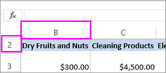
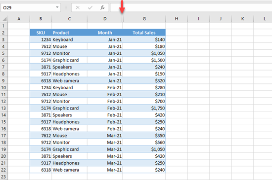
If you don’t see the first column (column A) or row (row 1) in your worksheet, it might be hidden. Here’s how to unhide it. In this picture column A and row 1 are hidden.

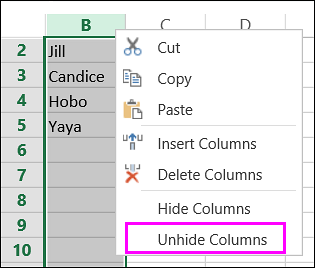
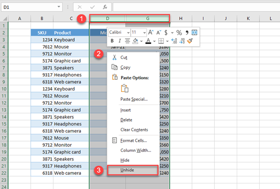
To unhide column A, right-click the column B header or label and pick Unhide Columns.

To unhide row 1, right-click the row 2 header or label and pick Unhide Rows.

Tip: If you don’t see Unhide Columns or Unhide Rows, make sure you’re right-clicking inside the column or row label.

Источник

Download Article

Are there hidden rows in your Excel worksheet that you want to bring back into view? Unhiding rows is easy, and you can even unhide multiple rows at once. This wikiHow article will teach you one or more rows in Microsoft Excel on your PC or Mac.

1

Open the Excel document. Double-click the Excel document that you want to use to open it in Excel.
2

Find the hidden row. Look at the row numbers on the left side of the document as you scroll down; if you see a skip in numbers (e.g., row 23 is directly above row 25), the row in between the numbers is hidden (in 23 and 25 example, row 24 would be hidden). You should also see a double line between the two row numbers.^[1]

Advertisement
3
Right-click the space between the two row numbers. Doing so prompts a drop-down menu to appear.
- For example, if row 24 is hidden, you would right-click the space between 23 and 25.
- On a Mac, you can hold down Control while clicking this space to prompt the drop-down menu.
4
Click Unhide. It’s in the drop-down menu. Doing so will prompt the hidden row to appear.
- You can save your changes by pressing Ctrl+S (Windows) or ⌘ Command+S (Mac).
5
Unhide a range of rows. If you notice that several rows are missing, you can unhide all of the rows by doing the following:
- Hold down Ctrl (Windows) or ⌘ Command (Mac) while clicking the row number above the hidden rows and the row number below the hidden rows.
- Right-click one of the selected row numbers.
- Click Unhide in the drop-down menu.

1

Open the Excel document. Double-click the Excel document that you want to use to open it in Excel.
2
Click the «Select All» button. This triangular button is in the upper-left corner of the spreadsheet, just above the 1 row and just left of the A column heading. Doing so selects your entire Excel document.
- You can also click any cell in the document and then press Ctrl+A (Windows) or ⌘ Command+A (Mac) to select the whole document.
3
Click the Home tab. This tab is just below the green ribbon at the top of the Excel window.
- If you’re already on the Home tab, skip this step.
4

Click Format. This option is in the «Cells» section of the toolbar near the top-right of the Excel window. A drop-down menu will appear.
5

Select Hide & Unhide. You’ll find this option in the Format drop-down menu. Selecting it prompts a pop-out menu to appear.
6
Click Unhide Rows. It’s in the pop-out menu. Doing so immediately causes any hidden rows to appear in the spreadsheet.
- You can save your changes by pressing Ctrl+S (Windows) or ⌘ Command+S (Mac).

1

Understand when this method is necessary. One form of hiding rows involves the height of the row(s) in question to be so short that the row effectively disappears. You can reset the height of all spreadsheet rows to «14.4» (the default height) to address this.
2

Open the Excel document. Double-click the Excel document that you want to use to open it in Excel.
3
Click the «Select All» button. This triangular button is in the upper-left corner of the spreadsheet, just above the 1 row and just left of the A column heading. Doing so selects your entire Excel document.
- You can also click any cell in the document and then press Ctrl+A (Windows) or ⌘ Command+A (Mac) to select the whole document.
4
Click the Home tab. This tab is just below the green ribbon at the top of the Excel window.
- If you’re already on the Home tab, skip this step.
5

Click Format. This option is in the «Cells» section of the toolbar near the top-right of the Excel window. A drop-down menu will appear.
6

Click Row Height…. It’s in the drop-down menu. This will open a pop-up window with a blank text field in it.
7

Enter the default row height. Type 14.4 into the pop-up window’s text field.
8
Click OK. Doing so will apply your changes to all rows in the spreadsheet, thus unhiding any rows which were «hidden» via their height properties.
- You can save your changes by pressing Ctrl+S (Windows) or ⌘ Command+S (Mac).

Add New Question

Question

The top 7 rows of my Excel worksheet have disappeared. I’ve tried to «unhide» from the Format menu, but nothing happens. What do I do?

You’ll have to unlock the cells (via the format pop-up), then hide them all before unhiding them.
Question

I have the same problem — top 7 rows aren’t displaying. I tried to unlock but they weren’t locked and the spreadsheet isn’t protected. I can see the top 7 rows only in print preview.

Anuj_Kumar1

Community Answer

There is a possibility you did not hide the rows but reduced your rows’ height to minimum. Select all rows above and below of your 7 rows and increase rows height from format menu. It will re-adjust the height of rows and your rows will be visible.

Ask a Question

200 characters left

Include your email address to get a message when this question is answered.

Submit

Thanks for submitting a tip for review!

About This Article

Article SummaryX

1. Open your spreadsheet in Microsoft Excel.
2. Select all data in the worksheet. A quick way to do this is to click the «»Select all»» button at the top-left corner of the worksheet.
3. Click the «»Home»» tab.
4. Click the «»Format»» button in the «»Cells»» section of the toolbar. A menu will expand.
5. Select «»Hide & Unhide»» on the menu.
6. Click «»Unhide rows»» to make all hidden rows visible.

Did this summary help you?

Thanks to all authors for creating a page that has been read 563,754 times.

Is this article up to date?

Источник

You can hide and unhide rows in Excel by right-clicking, or reveal all hidden rows using the «Format» option in the «Home» tab.
Hiding rows in Excel is especially helpful when working in large documents or for concealing information you won’t need until later.
Visit Business Insider’s homepage for more stories.

Just as you can quickly hide and unhide columns, you can hide or reveal hidden rows in your Excel spreadsheet as well.

In addition to freezing rows, you may find it helpful to conceal rows you are no longer using without permanently deleting the data from your spreadsheet. To later reveal the hidden cells, you can right-click to unhide individual rows.

You can also navigate to the «Format» option to unhide all hidden rows. This feature is especially helpful if you’ve hidden multiple rows throughout a large spreadsheet.

Here’s how to do both.

Check out the products mentioned in this article:

Microsoft Office (From $139.99 at Best Buy)

MacBook Pro (From $1,299.99 at Best Buy)

Microsoft Surface Pro X (From $999 at Best Buy)

How to hide individual rows in Excel

1. Open Excel.

2. Select the row(s) you wish to hide. Select an entire row by clicking on its number on the left hand side of the spreadsheet. Select multiple rows by clicking on the row number, holding the «Shift» key on your Mac or PC keyboard, and selecting another.

3. Right-click anywhere in the selected row.

4. Click «Hide.»

How to unhide rows in Excel

Right-click to hide rows.

Marissa Perino/Business Insider

How to unhide individual rows in Excel

1. Highlight the row on either side of the row you wish to unhide.

2. Right-click anywhere within these selected rows.

3. Click «Unhide.»

How to unhide rows in Excel

Highlight adjacent cells to unhide a hidden row.

Marissa Perino/Business Insider

4. You can also manually click or drag to expand a hidden row. Hidden rows are indicated by a thicker border line. Move your cursor over this line until it turns into a double bar with arrows. Double click to reveal or click and drag to manually expand the hidden row or rows. (If you’ve hidden multiple rows, you may have to do this multiple times.)

How to unhide all rows in Excel

1. To unhide all hidden rows in Excel, navigate to the «Home» tab.

2. Click «Format,» which is located towards the right hand side of the toolbar.

3. Navigate to the «Visibility» section. You’ll find options to hide and unhide both rows and columns.

4. Hover over «Hide & Unhide.»

5. Select «Unhide Rows» from the list. This will reveal all hidden rows, a feature especially helpful if you’ve hidden multiple rows throughout a large spreadsheet.

How to unhide rows in Excel

Unhide all rows.

Marissa Perino/Business Insider

Related coverage from How To Do Everything: Tech:

How to make a line graph in Microsoft Excel in 4 simple steps using data in your spreadsheet
How to add a column in Microsoft Excel in 2 different ways
How to hide and unhide columns in Excel to optimize your work in a spreadsheet
How to search for terms or values in an Excel spreadsheet, and use Find and Replace

Marissa Perino is a former editorial intern covering executive lifestyle. She previously worked at Cold Lips in London and Creative Nonfiction in Pittsburgh. She studied journalism and communications at the University of Pittsburgh, along with creative writing. Find her on Twitter: @mlperino.

Unhide the first column or row in a worksheet

If the first row (row 1) or column (column A) is not displayed in the worksheet, it is a little tricky to unhide it because there is no easy way to select that row or column. You can select the entire worksheet, and then unhide rows or columns ( Home tab, Cells group, Format button, Hide & Unhide command), but that displays all hidden rows and columns in your worksheet, which you may not want to do. Instead, you can use the Name box or the Go To command to select the first row and column.

To select the first hidden row or column on the worksheet, do one of the following:

In the Name Box next to the formula bar, type A1, and then press ENTER.

On the Home tab, in the Editing group, click Find & Select, and then click Go To. In the Reference box, type A1, and then click OK.

On the Home tab, in the Cells group, click Format.

Do one of the following:

Under Visibility, click Hide & Unhide, and then click Unhide Rows or Unhide Columns.

Under Cell Size, click Row Height or Column Width, and then in the Row Height or Column Width box, type the value that you want to use for the row height or column width.

Tip: The default height for rows is 15, and the default width for columns is 8.43.

If you don’t see the first column (column A) or row (row 1) in your worksheet, it might be hidden. Here’s how to unhide it. In this picture column A and row 1 are hidden.

To unhide column A, right-click the column B header or label and pick Unhide Columns.

To unhide row 1, right-click the row 2 header or label and pick Unhide Rows.

Tip: If you don’t see Unhide Columns or Unhide Rows, make sure you’re right-clicking inside the column or row label.

Источник

Unhide the first column or row in a worksheet

If the first row (row 1) or column (column A) is not displayed in the worksheet, it is a little tricky to unhide it because there is no easy way to select that row or column. You can select the entire worksheet, and then unhide rows or columns ( Home tab, Cells group, Format button, Hide & Unhide command), but that displays all hidden rows and columns in your worksheet, which you may not want to do. Instead, you can use the Name box or the Go To command to select the first row and column.

To select the first hidden row or column on the worksheet, do one of the following:

In the Name Box next to the formula bar, type A1, and then press ENTER.

On the Home tab, in the Editing group, click Find & Select, and then click Go To. In the Reference box, type A1, and then click OK.

On the Home tab, in the Cells group, click Format.

Do one of the following:

Under Visibility, click Hide & Unhide, and then click Unhide Rows or Unhide Columns.

Under Cell Size, click Row Height or Column Width, and then in the Row Height or Column Width box, type the value that you want to use for the row height or column width.

Tip: The default height for rows is 15, and the default width for columns is 8.43.

If you don’t see the first column (column A) or row (row 1) in your worksheet, it might be hidden. Here’s how to unhide it. In this picture column A and row 1 are hidden.

To unhide column A, right-click the column B header or label and pick Unhide Columns.

To unhide row 1, right-click the row 2 header or label and pick Unhide Rows.

Tip: If you don’t see Unhide Columns or Unhide Rows, make sure you’re right-clicking inside the column or row label.

Источник

How to hide and unhide rows in Excel

by Svetlana Cheusheva, updated on March 17, 2023

The tutorial shows three different ways to hide rows in your worksheets. It also explains how to show hidden rows in Excel and how to copy only visible rows.

If you want to prevent users from wandering into parts of a worksheet you don’t want them to see, then hide such rows from their view. This technique is often used to conceal sensitive data or formulas, but you may also wish to hide unused or unimportant areas to keep your users focused on relevant information.

On the other hand, when updating your own sheets or exploring inherited workbooks, you would certainly want to unhide all rows and columns to view all data and understand the dependencies. This article will teach you both options.

How to hide rows in Excel

As is the case with nearly all common tasks in Excel, there is more than one way to hide rows: by using the ribbon button, right-click menu, and keyboard shortcut.

Anyway, you begin with selecting the rows you’d like to hide:

To select one row, click on its heading.
To select multiple contiguous rows, drag across the row headings using the mouse. Or select the first row and hold down the Shift key while selecting the last row.
To select non-contiguous rows, click the heading of the first row and hold down the Ctrl key while clicking the headings of other rows that you want to select.

With the rows selected, proceed with one of the following options.

Hide rows using the ribbon

If you enjoy working with the ribbon, you can hide rows in this way:

Go to the Home tab >Cells group, and click the Format button.
Under Visibility, point to Hide & Unhide, and then select Hide Rows.

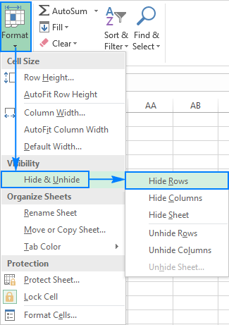
Alternatively, you can click Home tab >Format > Row Height… and type 0 in the Row Height box.

Either way, the selected rows will be hidden from view straight away.

In case you don’t want to bother remembering the location of the Hide command on the ribbon, you can access it from the context menu: right click the selected rows, and then click Hide.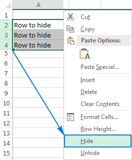

Excel shortcut to hide row

If you’d rather not take your hands off the keyboard, you can quickly hide the selected row(s) by pressing this shortcut: Ctrl + 9

How to unhide rows in Excel

As with hiding rows, Microsoft Excel provides a few different ways to unhide them. Which one to use is a matter of your personal preference. What makes the difference is the area you select to instruct Excel to unhide all hidden rows, only specific rows, or the first row in a sheet.

Unhide rows by using the ribbon

On the Home tab, in the Cells group, click the Format button, point to Hide & Unhide under Visibility, and then click Unhide Rows.

You select a group of rows including the row above and below the row(s) you want to unhide, right-click the selection, and choose Unhide in the pop-up menu. This method works beautifully for unhiding a single hidden row as well as multiple rows.

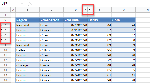
For example, to show all hidden rows between rows 1 and 8, select this group of rows like shown in the screenshot below, right-click, and click Unhide:

Unhide rows with a keyboard shortcut

Here is the Excel Unhide Rows shortcut: Ctrl + Shift + 9

Pressing this key combination (3 keys simultaneously) displays any hidden rows that intersect the selection.

Show hidden rows by double-clicking

In many situations, the fastest way to unhide rows in Excel is to double click them. The beauty of this method is that you don’t need to select anything. Simply hover your mouse over the hidden row headings, and when the mouse pointer turns into a split two-headed arrow, double click. That’s it!

How to unhide all rows in Excel

In order to unhide all rows on a sheet, you need to select all rows. For this, you can either:

Click the Select All button (a little triangle at the upper left corner of a sheet, in the intersection of the row and column headings):
Press the Select All shortcut: Ctrl + A

Please note that in Microsoft Excel, this shortcut behaves differently in different situations. If the cursor is in an empty cell, the whole worksheet is selected. But if the cursor is in one of contiguous cells with data, only that group of cells is selected; to select all cells, press Ctrl+A one more time.

Once the entire sheet is selected, you can unhide all rows by doing one of the following:

Press Ctrl + Shift + 9 (the fastest way).
Select Unhide from the right-click menu (the easiest way that does not require remembering anything).
On the Home tab, click Format >Unhide Rows (the traditional way).

How to unhide all cells in Excel

To unhide all rows and columns, select the whole sheet as explained above, and then press Ctrl + Shift + 9 to show hidden rows and Ctrl + Shift + 0 to show hidden columns.

How to unhide specific rows in Excel

Depending on which rows you want to unhide, select them as described below, and then apply one of the unhide options discussed above.

To show one or several adjacent rows, select the row above and below the row(s) that you want to unhide.
To unhide multiple non-adjacent rows, select all the rows between the first and last visible rows in the group.

For example, to unhide rows 3, 7, and 9, you select rows 2 — 10, and then use the ribbon, context menu or keyboard shortcut to unhide them.

How to unhide top rows in Excel

Hiding the first row in Excel is easy, you treat it just like any other row on a sheet. But when one or more top rows are hidden, how do you make them visible again, given that there is nothing above to select?

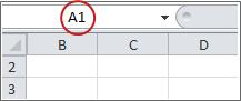
The clue is to select cell A1. For this, just type A1 in the Name Box, and press Enter.

Alternatively, go to the Home tab > Editing group, click Find & Select, and then click Go To… . The Go To dialog window pops up, you type A1 in the Reference box, and click OK.

With cell A1 selected, you can unhide the first hidden row in the usual way, by clicking Format > Unhide Rows on the ribbon, or choosing Unhide from the context menu, or pressing the unhide rows shortcut Ctrl + Shift + 9

Aside from this common approach, there is one more (and faster!) way to unhide first row in Excel. Simply hover over the hidden row heading, and when the mouse pointer turns into a split two-headed arrow, double click:

Tips and tricks for hiding and unhiding rows in Excel

As you have just seen, hiding and showing rows in Excel is quick and straightforward. In some situations, however, even a simple task can become a challenge. Below you will find easy solutions to a few tricky problems.

How to hide rows containing blank cells

To hide rows that contain any blank cells, proceed with these steps:

Select the range that contains empty cells you want to hide.
On the Home tab, in the Editing group, click Find & Select >Go To Special.
In the Go To Special dialog box, select the Blanks radio button, and click OK. This will select all empty cells in the range.
Press Ctrl + 9 to hide the corresponding rows.

This method works well when you want to hide all rows that contain at least one blank cell, as shown in the screenshot below:

If you want to hide blank rows in Excel, i.e. the rows where all cells are blank, then use the COUNTBLANK formula explained in How to remove blank rows to identify such rows.

How to hide rows based on cell value

To hide and show rows based on a cell value in one or more columns, use the capabilities of Excel Filter. It provides a handful of predefined filters for text, numbers and dates as well as an ability to configure a custom filter with your own criteria (please follow the above link for full details).

To unhide filtered rows, you remove filter from a specific column or clear all filters in a sheet, as explained here.

Hide unused rows so that only working area is visible

In situations when you have a small working area on the sheet and a whole lot of unnecessary blank rows and columns, you can hide unused rows in this way:

Select the row beneath the last row with data (to select the entire row, click on the row header).
Press Ctrl + Shift + Down arrow to extend the selection to the bottom of the sheet.
Press Ctrl + 9 to hide the selected rows.

In a similar fashion, you hide unused columns:

Select an empty column that comes after the last column of data.
Press Ctrl + Shift + Right arrow to select all other unused columns to the end of the sheet.
Press Ctrl + 0 to hide the selected columns. Done!

If you decide to unhide all cells later, select the entire sheet, then press Ctrl + Shift + 9 to unhide all rows and Ctrl + Shift + 0 to unhide all columns.

How to locate all hidden rows on a sheet

If your worksheet contains hundreds or thousands of rows, it can be hard to detect hidden ones. The following trick makes the job easy.

On the Home tab, in the Editing group, click Find & Select >Go To Special. Or press Ctrl+G to open the Go To dialog box, and then click Special.
In the Go To Special window, select Visible cells only and click OK.

This will select all visible cells and mark the rows adjacent to hidden rows with a white border:

How to copy visible rows in Excel

Supposing you have hidden a few irrelevant rows, and now you want to copy the relevant data to another sheet or workbook. How would you go about it? Select the visible rows with the mouse and press Ctrl + C to copy them? But that would also copy the hidden rows!

To copy only visible rows in Excel, you’ll have to go about it differently:

Select visible rows using the mouse.
Go to the Home tab >Editing group, and click Find & Select >Go To Special.
In the Go To Special window, select Visible cells only and click OK. That will really select only visible rows like shown in the previous tip.
Press Ctrl + C to copy the selected rows.
Press Ctrl + V to paste the visible rows.

Cannot unhide rows in Excel

If you have troubles unhiding rows in your worksheets, it’s most likely because of one of the following reasons.

1. The worksheet is protected

Whenever the Hide and Unhide features are disabled (greyed out) in your Excel, the first thing to check is worksheet protection.

For this, go to the Review tab > Changes group, and see if the Unprotect Sheet button is there (this button appears only in protected worksheets; in an unprotected worksheet, there will be the Protect Sheet button instead). So, if you see the Unprotect Sheet button, click on it.

If you want to keep the worksheet protection but allow hiding and unhiding rows, click the Protect Sheet button on the Review tab, select the Format rows box, and click OK.

Tip. If the sheet is password-protected, but you cannot remember the password, follow these guidelines to unprotect worksheet without password.

2. Row height is small, but not zero

In case the worksheet is not protected but specific rows still cannot be unhidden, check the height of those rows. The point is that if a row height is set to some small value, between 0.08 and 1, the row seems to be hidden but actually it is not. Such rows cannot be unhidden in the usual way. You have to change the row height to bring them back.

To have it done, perform these steps:

Select a group of rows, including a row above and a row below the problematic row(s).
Right click the selection and choose Row Height… from the context menu.
Type the desired number of the Row Height box (for example the default 15 points) and click OK.

This will make all hidden rows visible again.

If the row height is set to 0.07 or less, such rows can be unhidden normally, without the above manipulations.

3. Trouble unhiding the first row in Excel

If someone has hidden the first row in a sheet, you may have problems getting it back because you cannot select the row before it. In this case, select cell A1 as explained in How to unhide top rows in Excel and then unhide the row as usual, for example by pressing Ctrl + Shift + 9 .

4. Some rows are filtered out

When the row numbers in your worksheet turn blue, this indicates that some rows are filtered out. To unhide such rows, simply remove all filters on a sheet.

This is how you hide and undie rows in Excel. I thank you for reading and hope to see you on our blog next week!

Источник

Learn several ways to do this

Updated on September 19, 2022

What to Know

Hide a column: Select a cell in the column to hide, then press Ctrl+0. To unhide, select an adjacent column and press Ctrl+Shift+0.
Hide a row: Select a cell in the row you want to hide, then press Ctrl+9. To unhide, select an adjacent column and press Ctrl+Shift+9.
You can also use the right-click context menu and the format options on the Home tab to hide or unhide individual rows and columns.

You can hide columns and rows in Excel to make a cleaner worksheet without deleting data you might need later, although there is no way to hide individual cells. In this guide, we provide instructions for three ways to hide and unhide columns in Excel 2019, 2016, 2013, 2010, 2007, and Excel for Microsoft 365.

Hide Columns in Excel Using a Keyboard Shortcut

The keyboard key combination for hiding columns is Ctrl+0.

Click on a cell in the column you want to hide to make it the active cell.
Press and hold down the Ctrl key on the keyboard.
Press and release the 0 key without releasing the Ctrl key. The column containing the active cell should be hidden from view.

To hide multiple columns using the keyboard shortcut, highlight at least one cell in each column to be hidden, and then repeat steps two and three above.

Hide Columns Using the Context Menu

The options available in the context — or right-click menu — change depending upon the object selected when you open the menu. If the Hide option, as shown in the image below, is not available in the context menu it is likely that you didn’t select the entire column before right-clicking.

Hide a Single Column
Click the column header of the column you want to hide to select the entire column.
Right-click on the selected column to open the context menu.
Choose Hide. The selected column, the column letter, and any data in the column will be hidden from view.

Hide Adjacent Columns
In the column header, click and drag with the mouse pointer to highlight all three columns.
Right-click on the selected columns.
Choose Hide. The selected columns and column letters will be hidden from view.

When you hide columns and rows containing data, it does not delete the data, and you can still reference it in formulas and charts. Hidden formulas containing cell references will update if the data in the referenced cells changes.

Hide Separated Columns

In the column header click on the first column to be hidden.
Press and hold down the Ctrl key on the keyboard.
Continue to hold down the Ctrl key and click once on each additional column to be hidden to select them.
Release the Ctrl key.
In the column header, right-click on one of the selected columns and choose Hide. The selected columns and column letters will be hidden from view.

When hiding separate columns, if the mouse pointer is not over the column header when you click the right mouse button, the hide option will not be available.

Hide and Unhide Columns in Excel Using the Name Box

This method can be used to unhide any single column. In our example, we will be using column A.

Type the cell reference A1 into the Name Box.
Press the Enter key on the keyboard to select the hidden column.
Click on the Home tab of the ribbon.
Click on the Format icon on the ribbon to open the drop-down.
In the Visibility section of the menu, choose Hide & Unhide > Hide Columns or Unhide Column.

Unhide Columns Using a Keyboard Shortcut

The key combination for unhiding columns is Ctrl+Shift+0.

Type the cell reference A1 into the Name Box.
Press the Enter key on the keyboard to select the hidden column.
Press and hold down the Ctrl and the Shift keys on the keyboard.
Press and release the 0 key without releasing the Ctrl and Shift keys.

To unhide one or more columns, highlight at least one cell in the columns on either side of the hidden column(s) with the mouse pointer.

Click and drag with the mouse to highlight columns A to G.
Press and hold down the Ctrl and the Shift keys on the keyboard.
Press and release the 0 key without releasing the Ctrl and Shift keys. The hidden column(s) will become visible.

The Ctrl+Shift+0 keyboard shortcut might not work depending on the version of Windows you’re running, for reasons not explained by Microsoft. If this shortcut doesn’t work, use another method from the article.

Unhide Columns Using the Context Menu

As with the shortcut key method above, you must select at least one column on either side of a hidden column or columns to unhide them. For example, to unhide columns D, E, and G:
Hover the mouse pointer over column C in the column header. Click and drag with the mouse to highlight columns C to H to unhide all columns at one time.
Right-click on the selected columns and choose Unhide. The hidden column(s) will become visible.

Hide Rows Using Shortcut Keys

The keyboard key combination for hiding rows is Ctrl+9:

Click on a cell in the row you want to hide to make it the active cell.
Press and hold down the Ctrl key on the keyboard.
Press and release the 9 key without releasing the Ctrl key. The row containing the active cell should be hidden from view.

To hide multiple rows using the keyboard shortcut, highlight at least one cell in each row you want to hide, and then repeat steps two and three above.

Hide Rows Using the Context Menu

The options available in the context menu — or right-click — change depending upon the object selected when you open it. If the Hide option, as shown in the image above, is not available in the context menu it is because you probably didn’t select the entire row.

Hide a Single Row

Click on the row header for the row to be hidden to select the entire row.
Right-click on the selected row to open the context menu.
Choose Hide. The selected row, the row letter, and any data in the row will be hidden from view.

Hide Adjacent Rows

In the row header, click and drag with the mouse pointer to highlight all three rows.
Right-click on the selected rows and choose Hide. The selected rows will be hidden from view.

Hide Separated Rows

In the row header, click on the first row to be hidden.
Press and hold down the Ctrl key on the keyboard.
Continue to hold down the Ctrl key and click once on each additional row to be hidden to select them.
Right-click on one of the selected rows and choose Hide. The selected rows will be hidden from view.

Hide and Unhide Rows Using the Name Box

This method can be used to unhide any single row. In our example, we will be using row 1.

Type the cell reference A1 into the Name Box.
Press the Enter key on the keyboard to select the hidden row.
Click on the Home tab of the ribbon.
Click on the Format icon on the ribbon to open the drop-down menu.
In the Visibility section of the menu, choose Hide & Unhide > Hide Rows or Unhide Row.

Unhide Rows Using a Keyboard Shortcut

The key combination for unhiding rows is Ctrl+Shift+9.

Unhide Rows using Shortcut Keys and Name Box

Type the cell reference A1 into the Name Box.
Press the Enter key on the keyboard to select the hidden row.
Press and hold down the Ctrl and the Shift keys on the keyboard.
Press and hold down the Ctrl and the Shift keys on the keyboard. Row 1 will become visible.

Unhide Rows Using a Keyboard Shortcut

To unhide one or more rows, highlight at least one cell in the rows on either side of the hidden row(s) with the mouse pointer. For example, you want to unhide rows 2, 4, and 6.

To unhide all rows, click and drag with the mouse to highlight rows 1 to 7.
Press and hold down the Ctrl and the Shift keys on the keyboard.
Press and release the number 9 key without releasing the Ctrl and Shift keys. The hidden row(s) will become visible.

Unhide Rows Using the Context Menu

As with the shortcut key method above, you must select at least one row on either side of a hidden row or rows to unhide them. For example, to unhide rows 3, 4, and 6:

Hover the mouse pointer over row 2 in the row header.
Click and drag with the mouse to highlight rows 2 to 7 to unhide all rows at one time.
Right-click on the selected rows and choose Unhide. The hidden row(s) will become visible.

How to Move Columns in Excel

FAQ

How do I hide cells in Excel?

Select the cell or cells you want to hide, then select the Home tab > Cells > Format > Format Cells. In the Format Cells menu, select the Number tab > Custom (under Category) and type ;;; (three semicolons), then select OK.
How do I hide gridlines in Excel?

Select the Page Layout tab, then turn off the View checkbox under Gridlines.
How do I hide formulas in Excel?

Select the cells with formulas you want to hide > select the Hidden checkbox on the Protection tab > OK > Review > Protect Sheet. Next, verify that Protect worksheet and contents of locked cells is turned on, then select OK.

Thanks for letting us know!

Get the Latest Tech News Delivered Every Day

Источник

This Excel tutorial explains how to unhide row 1 in Excel 2016 (with screenshots and step-by-step instructions).

Question: How do I unhide row #1 in a sheet in Microsoft Excel 2016?

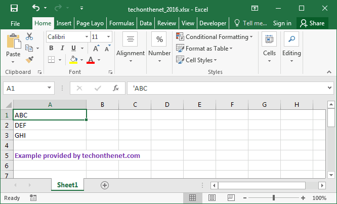
Answer: In this example, you can see that row 1 is hidden in the spreadsheet.

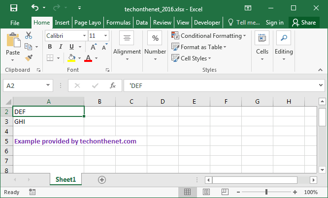
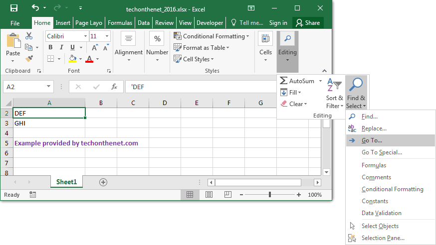
To unhide row 1, select the Home tab from the toolbar at the top of the screen. In the Editing group, click on Find & Select button and select «Go To…» from the popup menu.

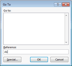
When the GoTo window appears, enter A1 in the Reference field and click on the OK button.

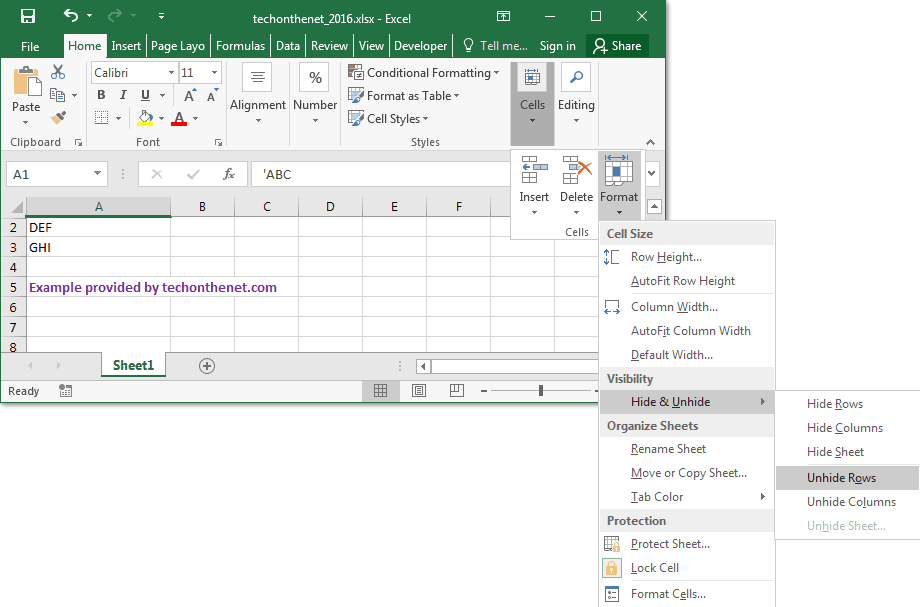
Select the Home tab from the toolbar at the top of the screen. Select Cells > Format > Hide & Unhide > Unhide Rows.

Row 1 should now be visible in the spreadsheet.

TIP: If you are unhiding rows 1-3 and the instructions above did not work. Try hiding rows 1-3 (even if they were hidden) and then try unhiding them again.

Источник

Bottom line: Learn some of my favorite keyboard shortcuts when working with rows and columns in Excel.

Skill level: Easy

Whether you are creating a simple list of names or building a complex financial model, you probably make a lot of changes to the rows and columns in the spreadsheet. Tasks like adding/deleting rows, adjusting column widths, and creating outline groups are very common when working with the grid.

This post contains some of my favorite shortcuts that will save you time every day.

I’ve also listed the equivalent shortcuts for the Mac version of Excel where available.

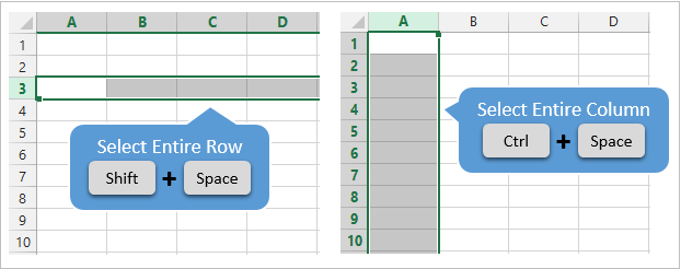
#1 – Select Entire Row or Column

Shift+Space is the keyboard shortcut to select an entire row.

Ctrl+Space is the keyboard shortcut to select an entire column.

Mac Shortcuts: Same as above

The keyboard shortcuts by themselves don’t do much. However, they are the starting point for performing a lot of other actions where you first need to select the entire row or column. This includes tasks like deleting rows, grouping columns, etc.

These shortcuts also work for selecting the entire row or column inside an Excel Table.

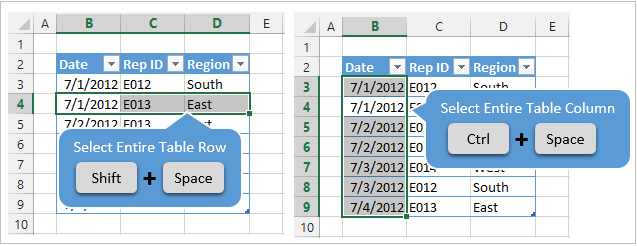
When you press the Shift+Space shortcut the first time it will select the entire row within the Table. Press Shift+Space a second time and it will select the entire row in the worksheet.

The same works for columns. Ctrl+Space will select the column of data in the Table. Pressing the keyboard shortcut a second time will include the column header of the Table in the selection. Pressing Ctrl+Space a third time will select the entire column in the worksheet.

You can select multiple rows or columns by holding Shift and pressing the Arrow Keys multiple times.

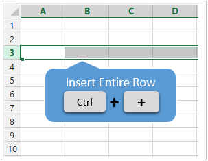
#2 – Insert or Delete Rows or Columns

There are a few ways to quickly delete rows and columns in Excel.

If you have the rows or columns selected, then the following keyboard shortcuts will quickly add or delete all selected rows or columns.

Ctrl++ (plus character) is the keyboard shortcut to insert rows or columns. If you are using a laptop keyboard you can press Ctrl+Shift+= (equal sign).

Mac Shortcut: Cmd++ or Cmd+Shift+

Ctrl+- (minus character) is the keyboard shortcut to delete rows or columns.

Mac Shortcut: Cmd+-

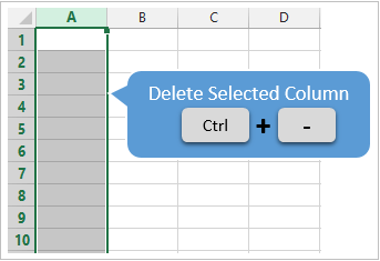
So for the above shortcuts to work you will first need to select the entire row or column, which can be done with the Shift+Space or Ctrl+Space shortcuts explained in #1.

If you do not have the entire row or column selected then you will be presented with the Insert or Delete Menus after pressing Ctrl++ or Ctrl+-.

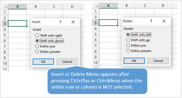
You can then press the up or down arrow keys to make your selection from the menu and hit Enter. For me it is easier to first select the entire row or column, then press Ctrl++ or Ctrl+-.

So, the entire keyboard shortcut to delete a column would be Ctrl+Space, Ctrl+-. You could also use the keyboard shortcut Alt+H+D+C to delete columns and Alt+H+D+R to delete rows. There are lots of ways to do a simple task… 🙂

#3 – AutoFit Column Width

There are also a lot of different ways to AutoFit column widths. AutoFit means that the width of the column will be adjusted to fit the contents of the cell.

You can use the mouse and double-click when you hover the cursor between columns when you see the resize column cursor.

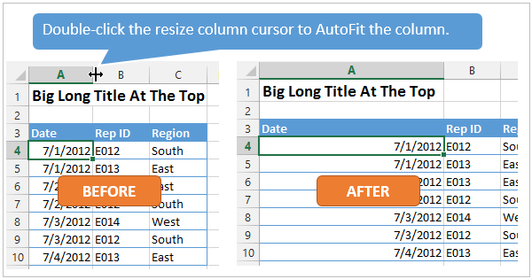
The problem with this is that you might just want to resize the column for the date in cell A4, instead of the big long title in cell A1. To accomplish this you can use the AutoFit Column Width button. It is located on the Home tab of the Ribbon in the Format menu.

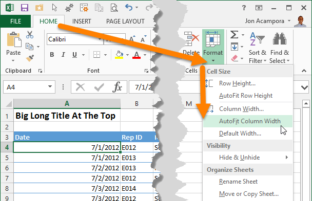
The AutoFit Column Width button bases the width of the column on the cells you have selected. In the image above I have cell A4 selected. So the column width will be adjusted to fit the contents of A4, as shown in the results below.

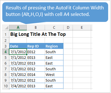
Alt,H,O,I is the keyboard shortcut for the AutoFit Column Width button. This is one I use a lot to get my reports looking shiny. 🙂

Alt,H,O,A is the keyboard shortcut to AutoFit Row Height. It doesn’t work exactly the same as column width, and will only adjust the row height to the tallest cell in the entire row.

Mac Shortcuts: None that I know of. The Mac version does not use the Alt key sequence which I believe is a limitation of the Mac OS.

#3.5 – Manually Adjust Row or Column Width

The column width or row height windows can be opened with keyboard shortcuts as well.

Alt,O,R,E is the keyboard shortcut to open the Row Height window.

Alt,O,C,W is the keyboard shortcut to open the Column Width window.

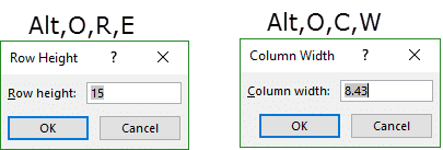
The row height or column width will be applied to the rows or columns of all the cells that are currently selected.

These are old shortcuts from Excel 2003, but they still work in the modern versions of Excel.

Mac Shortcuts: None that I know of. The Mac version does not use the Alt key sequence which I believe is a limitation of the Mac OS.

#4 – Hide or Unhide Rows or Columns

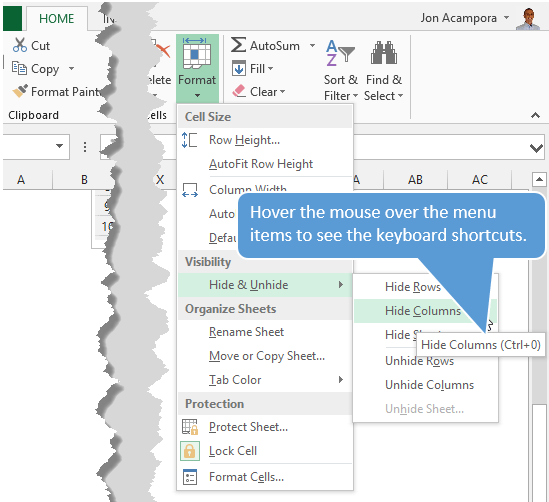
There are several dedicated keyboard shortcuts to hide and unhide rows and columns.

Ctrl+9 to Hide Rows
Ctrl+0 (zero) to Hide Columns
Ctrl+Shift+( to Unhide Rows
Ctrl+Shift+) to Unhide Columns – If this doesn’t work for you try Alt,O,C,U (old Excel 2003 shortcut that still works). You can also modify a Windows setting to prevent the conflict with this shortcut. See the comment from Pablo Baez on Oct 5, 2015 below for further instructions. Thanks Pablo! 🙂

Mac Shortcuts: Same as above

The buttons are also located on the Format menu on the Home tab of the Ribbon. You can hover over any of the items in the menu and the keyboard shortcut will display in the screentip (see screenshot below).

The trick with getting these shortcuts to work is to have the proper cells selected first.

To hide rows or columns you just need to select cells in the rows or columns you want to hide, then press the Ctrl+9 or Ctrl+Shift+( shortcut.

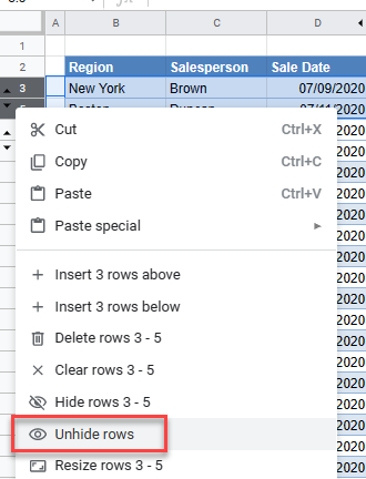
To unhide rows or columns you first need to select the cells that surround the rows or columns you want to unhide. In the screenshot below I want to unhide rows 3 & 4. I first select cell B2:B5, cells that surround or cover the hidden rows, then press Ctrl+Shift+( to unhide the rows.

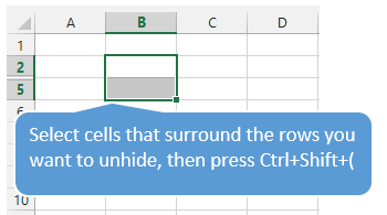
The same technique works to unhide columns.

#5 – Group or Ungroup Rows or Columns

Row and Column groupings are a great way to quickly hide and unhide columns and rows.

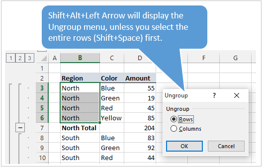
Shift+Alt+Right Arrow is the shortcut to group rows or columns.

Mac Shortcut: Cmd+Shift+K

Shift+Alt+Left Arrow is the shortcut to ungroup.

Mac Shortcut: Cmd+Shift+J

Again, the trick here is to select the entire rows or columns you want to group/ungroup first. Otherwise you will be presented with the Group or Ungroup menu.

Alt,A,U,C is the keyboard shortcut to remove all the row and columns groups on the sheet. This is the same as pressing the Clear Outline button on the Ungroup menu of the Data tab on the Ribbon.

*Bonus funny: At some point when using the group/ungroup shortcuts, you will accidentally press Ctrl+Alt+Right Arrow. This is a Windows shortcut that orientates the entire screen to the right. I call it “neck ache view”. To get it back to normal press Ctrl+Alt+Up Arrow.

If your co-worker or boss accidentally leaves their computer unlocked and you want to play a joke on them, press Ctrl+Alt+Down Arrow. This will turn their screen upside down. Don’t forget to record a video of their WTF reaction… 🙂

What Are Your Favorites?

There are a ton of keyboard shortcuts for working with rows and columns. The above are some of my favorites that I use everyday. What are some of your favorites? Please leave a comment below. Thanks! 🙂

Источник

See all How-To Articles

This tutorial demonstrates how to hide and unhide rows and columns in Excel and Google Sheets.

There are several ways to limit which rows and columns are visible in an Excel spreadsheet. This tutorial shows how to use hide and unhide them. Other options include VBA or Excel’s Outline feature.

Hide and Unhide Rows

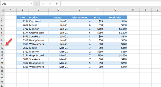
Let’s start with the example below, a set of sales data, to show how to hide and unhide rows or columns.

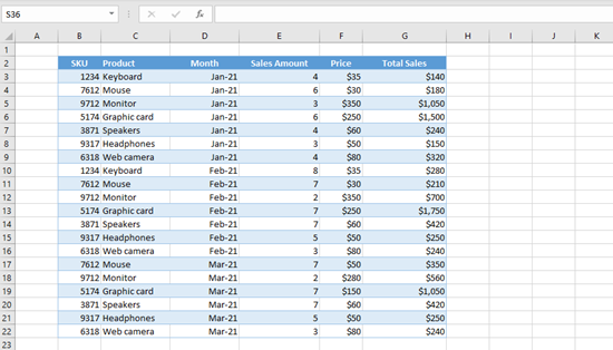
Let’s, for example, hide all rows for Feb-21 (10–16).

Click and hold the Row 10 heading and drag through Row 16 to select Rows 10 to 16. (You could, alternatively, select Row 10, hold SHIFT, and select Row 16.)
Then, right-click anywhere in the selected range.
Click Hide.

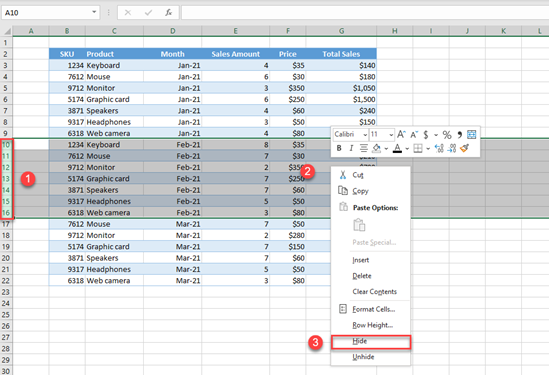
As a result, Rows 10–16 are hidden, and you can’t see them in the worksheet.

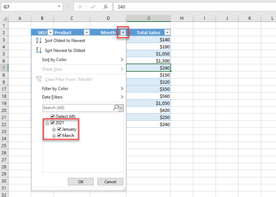
If you try to filter data by Month now (Column D), we’ll see that only values that are not hidden are displayed (Jan-21 and Mar-21) and Feb-21, which is hidden, is not shown.

Unhide Rows

You can then unhide these rows to display them again.

First, select one row before and one row after the hidden rows (9 and 17).
Right-click somewhere in the selected range.
Choose Unhide.

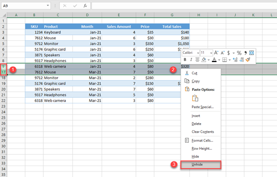
Now, Rows 10–16 are unhidden, and you can see them again.

Hide and Unhide Columns

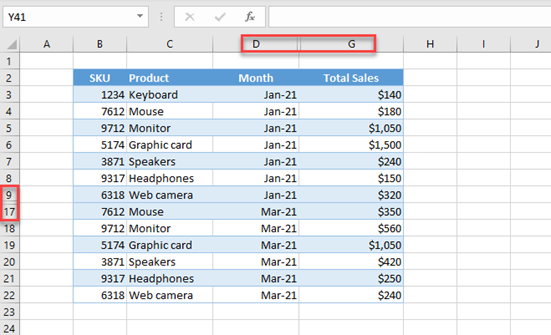
Hiding and unhiding columns work like hiding rows. Only, instead of row numbers, use column headings. Say you want to hide Sales Amount and Price from the sheet (Columns E and F).

Click and hold the Column E heading and drag to Column F; this selects Columns E and F.
Then, right-click anywhere in the selected range.
Click Hide.

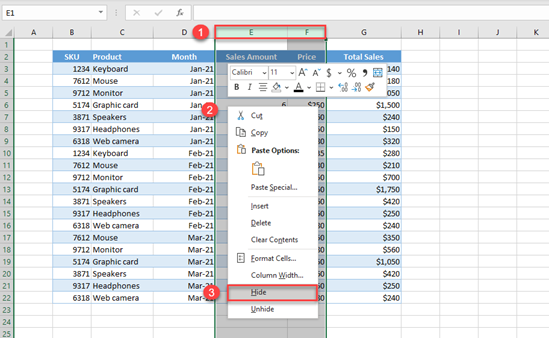
As a result, Columns E and F are hidden, and you can’t see them in the worksheet.

Unhide Columns

You can then unhide these two columns to display them again.

First, select one column before and one column after the hidden columns (D and G).
Right-click somewhere in the selected range.
Choose Unhide.

Finally, Columns E and F are unhidden, and you can see them again.

To hide entire sheets, see How to Hide and Unhide Worksheets in Excel and Google Sheets. Or hide an entire workbook.

Hide and Unhide Rows and Columns in Google Sheets

Hiding and unhiding rows and columns work exactly the same in Google Sheets.

Select the row above and the row below the hidden row or rows and right-click. Click Unhide rows to show the hidden row or rows.

Источник

Hide and Unhide Rows and Columns in Microsoft Excel (with Shortcuts)

by Avantix Learning Team | Updated January 29, 2022

Applies to: Microsoft^® Excel^® 2013, 2016, 2019 and 365 (Windows)

You can hide or unhide columns or rows in Excel using the context menu, using a keyboard shortcut or by using the Format command on the Home tab in the Ribbon. You can quickly unhide all columns or rows as well.

Some users may want to hide all of the unused columns to the right and unused rows below the data to clean up the workspace and display only relevant information to team members or clients.

You will not be able to hide or unhide rows or columns if the worksheet has been protected with a password (and you don’t have the password to unprotect it), if content has been disabled or if the file is read only.

Recommended article: How to Lock and Protect Excel Worksheets and Workbooks

Selecting columns or rows in Excel

It’s important to be able to quickly select columns or rows in Excel if you want to hide them.

To select one or more columns in Excel:

To select one column, click its heading or select a cell in the column and press Ctrl + spacebar.
To select multiple contiguous columns, drag across the column headings using a mouse or select the first column and then Shift-click the last column.
To select non-contiguous columns, click the heading of the first column and then Ctrl-click the headings or the other columns you want to select.

To select one or more rows in Excel:

To select one row, click its heading or select a cell in the row and press Shift + Spacebar.
To select multiple contiguous rows, drag across the row headings using a mouse or select the first row and then Shift-click the last row.
To select non-contiguous rows, click the heading of the first row and then Ctrl-click the headings of the other rows you want to select.

To select all rows and columns in Excel:

Press Ctrl + A (press A twice if necessary).
Click in the intersection box to the left of the A and above the 1 on the worksheet.

Hiding columns

To hide a column or columns by right-clicking:

Select the column or columns you want to hide.
Right-click and select Hide from the drop-down menu.

To hide a column or columns using a keyboard shortcut:

Select the column or columns you want to hide.
Press Ctrl + 0 (zero).

To hide a column or columns using the Ribbon:

Select the column or columns you want to hide.
Click the Home tab in the Ribbon.
In the Cells group, click Format. A drop-down menu appears.
Click Visibility, select Hide & Unhide and then Hide Columns.

To hide all columns to the right of the last line of data:

Select the column to the right of the last column of data.
Press Ctrl + Shift + right arrow.
Press Ctrl + 0 (zero). You can also use the Ribbon method or the right-click method to hide columns.

Unhiding columns

To unhide a column or columns by right-clicking:

Select the column headings to the left and right of the hidden column(s). To unhide all columns, click the box to the left of the A and above the 1 on the worksheet or press Ctrl + A (twice if necessary).
Right-click and select Unhide from the drop-down menu.

To unhide a column or columns using a keyboard shortcut:

Select the column headings to the left and right of the hidden column(s) by dragging. To unhide all columns, click the box to the left of the A and above the 1 on the worksheet or press Ctrl + A (twice if necessary).
Press Ctrl + Shift + 0 (zero). If this doesn’t work, use one of the other methods.

To unhide a column or columns using the Ribbon:

Select the column headings to the left and right of the hidden column(s). To select all columns, click the box to the left of the A and above the 1 on the worksheet or press Ctrl + A (twice if necessary).
Click the Home tab in the Ribbon.
In the Cells group, click Format. A drop-down menu appears.
Click Visibility, select Hide & Unhide and then Unhide Columns.

To unhide a column or columns by double-clicking:

Select the column headings to the left and right of the hidden columns(s).
Hover the mouse over the hidden column headings.
When the mouse pointer turns into a split two-headed arrow, double-click.

Hiding rows

To hide a row or rows by right-clicking:

Select the row or rows you want to hide.
Right-click and select Hide from the drop-down menu.

To hide a row or rows using a keyboard shortcut:

Select the row or rows you want to hide.
Press Ctrl + 9.

To hide a row or rows using the Ribbon:

Select the row or rows you want to hide.
Click the Home tab in the Ribbon.
In the Cells group, click Format. A drop-down menu appears.
Click Visibility, select Hide & Unhide and then Hide Rows.

To hide all rows below the last line of data:

Select the row below the last line of data.
Press Ctrl + Shift + down arrow.
Press Ctrl + 9. You can also use the Ribbon method or the right-click method to hide the rows.

Unhiding rows

To unhide a row or rows by right-clicking:

Select the row headings above and below the hidden row(s). To unhide all rows, click the box to the left of the A and above the 1 on the worksheet.
Right-click and select Unhide from the drop-down menu.

To unhide rows using a keyboard shortcut:

Select the row headings above and below the hidden row(s). To unhide all rows, click the box to the left of the A and above the 1 on the worksheet or press Ctrl + A (twice if necessary).
Press Ctrl + Shift + 9.

To unhide a row or rows using the Ribbon:

Select the row headings above and below the hidden row(s). To select all rows, click the box to the left of the A and above the 1 on the worksheet.
Click the Home tab in the Ribbon or press Ctrl + A (twice if necessary).
In the Cells group, click Format. A drop-down menu appears.
Click Visibility, select Hide & Unhide and then Unhide Rows.

To unhide a row or rows by double-clicking:

Select the row headings above and below the hidden row(s). To unhide all rows, click the box to the left of the A and above the 1 on the worksheet.
Hover the mouse over the hidden row headings.
When the mouse pointer turns into a split two-headed arrow, double-click.

The method you use to hide or unhide columns or rows is based on personal preference.

Subscribe to get more articles like this one

Did you find this article helpful? If you would like to receive new articles, join our email list.

More resources

How to Convert Text to Numbers in Excel (5 Ways)

How to Use Flash Fill in Excel (4 Ways with Shortcuts)

10 Ways to Save Time Selecting in Excel using the Name Box

How to Delete Blank Rows in Excel (5 Easy Ways with Shortcuts)

How to Highlight Errors, Blanks and Duplicates in Excel Worksheets (Using Formulas)

Related courses

Microsoft Excel: Intermediate / Advanced

Microsoft Excel: Data Analysis with Functions, Dashboards and What-If Analysis Tools

Microsoft Excel: Introduction to Visual Basic for Applications (VBA)

VIEW MORE COURSES >

Our instructor-led courses are delivered in virtual classroom format or at our downtown Toronto location at 18 King Street East, Suite 1400, Toronto, Ontario, Canada (some in-person classroom courses may also be delivered at an alternate downtown Toronto location). Contact us at info@avantixlearning.ca if you’d like to arrange custom instructor-led virtual classroom or onsite training on a date that’s convenient for you.

Microsoft, the Microsoft logo, Microsoft Office and related Microsoft applications and logos are registered trademarks of Microsoft Corporation in Canada, US and other countries. All other trademarks are the property of the registered owners.

Avantix Learning |18 King Street East, Suite 1400, Toronto, Ontario, Canada M5C 1C4 | Contact us at info@avantixlearning.ca

Источник

About This Article

Is this article up to date?

Check out the products mentioned in this article:

Microsoft Office (From $139.99 at Best Buy)

MacBook Pro (From $1,299.99 at Best Buy)

Microsoft Surface Pro X (From $999 at Best Buy)

How to hide individual rows in Excel

How to unhide individual rows in Excel

How to unhide all rows in Excel

Related coverage from How To Do Everything: Tech:

How to make a line graph in Microsoft Excel in 4 simple steps using data in your spreadsheet

How to add a column in Microsoft Excel in 2 different ways

How to hide and unhide columns in Excel to optimize your work in a spreadsheet

How to search for terms or values in an Excel spreadsheet, and use Find and Replace

Unhide the first column or row in a worksheet

Unhide the first column or row in a worksheet

How to hide and unhide rows in Excel

How to hide rows in Excel

Hide rows using the ribbon

Excel shortcut to hide row

How to unhide rows in Excel

Unhide rows by using the ribbon

Unhide rows with a keyboard shortcut

Show hidden rows by double-clicking

How to unhide all rows in Excel

How to unhide all cells in Excel

How to unhide specific rows in Excel

How to unhide top rows in Excel

Tips and tricks for hiding and unhiding rows in Excel

How to hide rows containing blank cells

How to hide rows based on cell value

Hide unused rows so that only working area is visible

How to locate all hidden rows on a sheet

How to copy visible rows in Excel

Cannot unhide rows in Excel

1. The worksheet is protected

2. Row height is small, but not zero

3. Trouble unhiding the first row in Excel

4. Some rows are filtered out

What to Know

Hide Columns in Excel Using a Keyboard Shortcut

Hide Columns Using the Context Menu

Hide a Single Column

Hide Adjacent Columns

Hide Separated Columns

Hide and Unhide Columns in Excel Using the Name Box

Unhide Columns Using a Keyboard Shortcut

Unhide Columns Using the Context Menu

Hide Rows Using Shortcut Keys

Hide Rows Using the Context Menu

Hide a Single Row

Hide Adjacent Rows

Hide Separated Rows

Hide and Unhide Rows Using the Name Box

Unhide Rows Using a Keyboard Shortcut

Unhide Rows using Shortcut Keys and Name Box

Unhide Rows Using a Keyboard Shortcut

Unhide Rows Using the Context Menu

#1 – Select Entire Row or Column

#2 – Insert or Delete Rows or Columns

#3 – AutoFit Column Width

#3.5 – Manually Adjust Row or Column Width

#4 – Hide or Unhide Rows or Columns

#5 – Group or Ungroup Rows or Columns

What Are Your Favorites?

Hide and Unhide Rows

Unhide Rows

Hide and Unhide Columns

Unhide Columns

Hide and Unhide Rows and Columns in Google Sheets

Hide and Unhide Rows and Columns in Microsoft Excel (with Shortcuts)

Selecting columns or rows in Excel

Hiding columns

Unhiding columns

Hiding rows

Unhiding rows

Subscribe to get more articles like this one

More resources

Related courses