У notation in excel - Word и Excel - помощь в работе с программами

Excel for Microsoft 365 Excel 2021 Excel 2019 Excel 2016 Excel 2013 Excel 2010 Excel 2007 More…Less

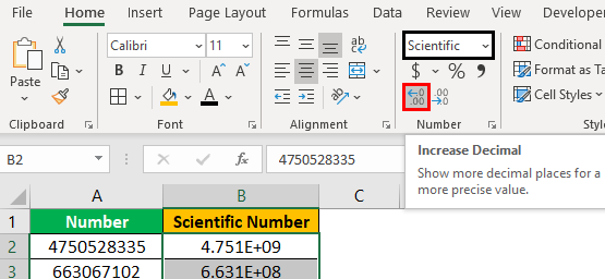
The Scientific format displays a number in exponential notation, replacing part of the number with E+n, in which E (exponent) multiplies the preceding number by 10 to the nth power. For example, a 2-decimal scientific format displays 12345678901 as 1.23E+10, which is 1.23 times 10 to the 10th power.

Follow these steps to apply the scientific format to a number.

Select the cells that you want to format. For more information, see Select cells, ranges, rows, or columns on a worksheet.

Tip: To cancel a selection of cells, click any cell on the worksheet.
On the Home tab, click the small More button next to Number.
In the Category list, click Scientific.
Using the small arrows, specify the Decimal places that you want to display.

Tip: The number that is in the active cell of the selection on the worksheet appears in the Sample box so that you can preview the number formatting options that you select.

Also, remember that:

To quickly format a number in scientific notation, click Scientific in the Number Format box (Home tab, Number group). The default for scientific notation is two decimal places.
A number format does not affect the actual cell value that Excel uses to perform calculations. The actual value can be seen in the formula bar.
The maximum limit for number precision is 15 digits, so the actual value shown in the formula bar may change for large numbers (more than 15 digits).
To reset the number format, click General in the Number Format box (Home tab, Number group). Cells that are formatted with the General format do not use a specific number format. However, the General format does use exponential notation for large numbers (12 or more digits). To remove the exponential notation from large numbers, you can apply a different number format, such as Number.

Need more help?

Want more options?

Explore subscription benefits, browse training courses, learn how to secure your device, and more.

Communities help you ask and answer questions, give feedback, and hear from experts with rich knowledge.

Источник

In this lesson, you will learn how to disable scientific notation (e.g., 1,23457E+17) in an Excel spreadsheet.

Table of content

How to format the cell to disable scientific notation?

Increasing the number of decimal places

Using the Custom format

Using the ROUND formula

How to concatenate the cell to disable scientific notation?

Using the Text to Columns Tool

Conversion of the cell to disable scientific notation

Trimming to remove scientific notation

Using the IF function

Using the FIX function

Using the INT function

Using the Trunc function

Pasting values as text

This problem exists when you want to paste a long number. Pasting it to the spreadsheet, Excel changes the formatting to scientific notation (e.g. 1,23457E+17).

This problem is caused by Excel, which has a 15-digit precision limit. It’s annoying, because most of the time, I’d prefer it if Excel just treated the number as text (until I wanted it sorted). You can solve this problem.

How to format the cell to disable scientific notation?

Just right click on the cell and choose Format cell.

Change the format from General to Number with a zero number of decimal places.

Now this problem doesn’t exist any more.

Tips:

This solution works for other types of formatting as well. For example, Custom with a single 0 or Text.
The number format does not affect the actual cell value, which is displayed in the formula bar.
When Excel displays a cell with #### signs, it means that the cell is too narrow. Just make it wider.

Increasing the number of decimal places

Increasing the number of decimal places is one of the simplest and most straightforward ways to disable scientific notation in Excel. Here’s how to do it:

Right-click on the cell that contains the number in scientific notation.
Select «Format Cells» from the context menu.
In the Format Cells dialog box, select the «Number» tab.
In the «Number» section, select the number of decimal places you want to display. The default is 2 decimal places, but you can increase this number to show more decimal places if necessary.
Click «OK» to apply the changes. The number will be displayed in the specified number of decimal places, instead of in scientific notation.

Note: This method works best for numbers that are small enough to be displayed with the specified number of decimal places. If the number is too large, it may still be displayed in scientific notation even if you increase the number of decimal places. In such cases, you may need to use a different method, such as changing the cell format to «Text» or using the «Text» formula.

Using the Custom format

Using the «Custom» format is another way to disable scientific notation in Excel. This method involves specifying a custom format for the cell to display the number in a specific way. Here’s how to do it:

Right-click on the cell that contains the number in scientific notation.
Select «Format Cells» from the context menu.
In the Format Cells dialog box, select the «Number» tab.
In the «Category» section, select «Custom.»
In the «Type» field, enter a custom format for the number. For example, to display the number with no decimal places, enter «0». To display the number with 2 decimal places, enter «0.00».
Click «OK» to apply the changes. The number will be displayed in the specified format, instead of in scientific notation.

Note: This method can be useful when you need to display a specific number of decimal places or when you want to display the number in a specific way (such as with a comma separator).

Using the ROUND formula

Using the «Round» formula is a way to disable scientific notation in Excel by rounding the number to a specified number of decimal places. Here’s how to do it:

Select the cell where you want to display the rounded number.
Enter the formula =ROUND(A1,0), where A1 is the cell that contains the number in scientific notation, and 0 is the number of decimal places you want to round to.
Press «Enter» to apply the formula. The number in cell A1 will be rounded to the specified number of decimal places and displayed in the selected cell.

Note: The «Round» formula is a useful method when you want to display the number in a simplified form with a specified number of decimal places. However, be aware that rounding can result in the loss of precision, and it may not be suitable for all purposes.

How to concatenate the cell to disable scientific notation?

The other way is to concatenate the cells to display the full content of each cell.

A simple =CONCATENATE(A1) formula would do the trick. Thanks to that trick, you will not see «E+» any more.

It worked because that is how the concatenate function works. As an output, it creates a single string, and Excel does not apply scientific notation to such a string. It is worth mentioning that it does not change the format of the cell.

You can also remove scientific notation with the Text to Columns tool. This tool is used to improve the content of cells in case of problems with their content or formatting.

To start, select the column that contains unnecessary scientific notations and go to the Excel ribbon. Click Data > Text to Columns.

In the first step, check the Fixed width option. Already at this stage you can see in the preview of selected data at the bottom of the window that scientific notation will be deleted.

In the third step, select the text from available Excel data types. When you click finish, the scientific notation will disappear from the cells.

The inconvenience is that green triangles will appear in the cells. If they bother you, check this link on how to remove green triangles from a spreadsheet in Excel.

Conversion of the cell to disable scientific notation

There is one more tricky way to accomplish the expected output that I would like to share with you.

There is a way to convert the content of the cell to the specific number format without changing it. Excel would stop using the scientific notation as well. This is the TEXT function that you need to use for that purpose.

=TEXT(A1,»0″) is the Excel formula you should use.

The result is the same. «E+» disappeared from the cell.

Trimming to remove scientific notation

Another way to remove scientific notation from your workbook is to use the trim function.

The Trim function is used to remove excess spaces from a cell. Using the formula Trim only leaves single spaces between words.

As a side effect of using the Trim formula, you will get rid of scientific notation.

Use the formula = TRIM (A1) to get rid of scientific notation.

Using the IF function

Using the «IF» formula is a way to disable scientific notation in Excel by evaluating the number and displaying it in either scientific notation or a custom format. Here’s how to do it:

Select the cell where you want to display the number.
Enter the formula =IF(ABS(A1)<1,»0.00″,A1), where A1 is the cell that contains the number in scientific notation.
Press «Enter» to apply the formula. The formula will evaluate the number in cell A1 and determine whether it is less than 1. If it is less than 1, it will display the number in a custom format with two decimal places. If it is not less than 1, it will display the number in its original format.

Note: This method is useful when you want to display the number in a custom format based on its value. However, be aware that the custom format may not be suitable for all purposes, and you may need to modify the formula to meet your specific needs.

Using the FIX function

Using the «FIX» formula is a way to disable scientific notation in Excel by rounding the number down to a specified number of decimal places. Here’s how to do it:

Select the cell where you want to display the rounded number.
Enter the formula =FIX(A1,n), where A1 is the cell that contains the number in scientific notation and n is the number of decimal places you want to round down to.
Press «Enter» to apply the formula. The number in cell A1 will be rounded down to the specified number of decimal places, and scientific notation will be disabled.

Note: This method is useful when you want to round the number and display it in a more readable format.

Using the INT function

Using the «INT» formula is a way to disable scientific notation in Excel by rounding the number down to the nearest integer. Here’s how to do it:

Select the cell where you want to display the rounded number.
Enter the formula =INT(A1), where A1 is the cell that contains the number in scientific notation.
Press «Enter» to apply the formula. The number in cell A1 will be rounded down to the nearest integer, and scientific notation will be disabled.

Note: This method is useful when you want to round the number and display it as a whole number.

Using the TRUNC function

Using the «TRUNC» formula is a way to disable scientific notation in Excel by truncating the number to a specified number of decimal places. Here’s how to do it:

Select the cell where you want to display the truncated number.
Enter the formula =TRUNC(A1,n), where A1 is the cell that contains the number in scientific notation and n is the number of decimal places you want to keep.
Press «Enter» to apply the formula. The number in cell A1 will be truncated to the specified number of decimal places, and scientific notation will be disabled.

Note: This method is useful when you want to remove the decimal portion of the number and display it as a whole number or a number with a limited number of decimal places.

Pasting values as text

Pasting values as text is a way to disable scientific notation in Excel by converting the number to text. Here’s how to do it:

Select the cells that contain the numbers in scientific notation.
Right-click the selected cells and choose «Copy».
Right-click the target cell where you want to paste the copied numbers and choose «Paste Special».
In the «Paste Special» dialog box, select «Values» and «Text» as the paste options.
Click «OK» to apply the paste operation. The numbers in scientific notation will be converted to text and scientific notation will be disabled.

Note: This method is useful when you want to preserve the original format of the numbers and prevent them from being changed by Excel.

In conclusion, there are several methods to disable scientific notation in Excel, including changing the cell format, using custom formats, using the «ROUND» formula, using the «FIX» formula, using the «INT» formula, using the «TRUNC» formula, using the «TEXT» formula, pasting values as text, and others. The best method to use will depend on your specific needs and requirements. If you need to perform mathematical calculations with the numbers, then you may need to use a different method than if you simply want to preserve the format of the numbers. Whatever method you choose, it’s important to understand how it works and how it can impact your data so that you can make informed decisions and achieve the desired result.

Further reading: 
Custom number format
Turning Off the Automatic Formatting of Dates
How to Exchange Formula to Value?
Excel interview questions

Источник

Scientific notation in Excel is a special way of writing small and large numbers, which helps us compare and use the same in calculations.

Excel Scientific Notation
- How to Format Scientific Notation in Excel? (with Examples)
  - Example #1 – For Positive Exponent
  - Example #2 – For Negative Exponent
- Things to Remember
- Recommended Articles

How to Format Scientific Notation in Excel? (with Examples)

You can download this Scientific Notation Excel Template here – Scientific Notation Excel Template

Example #1 – For Positive Exponent

Now, we will see how to work on Excel with scientific notation formatting. Below is the data for this example that we use. Please copy the above number list and paste it into your worksheet area.

Copy and paste the first column numbers to the next column.

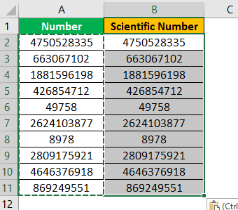
Now, by selecting the range, click on the dropdown list in excelA drop-down list in excel is a pre-defined list of inputs that allows users to select an option.read more in “Number” format.

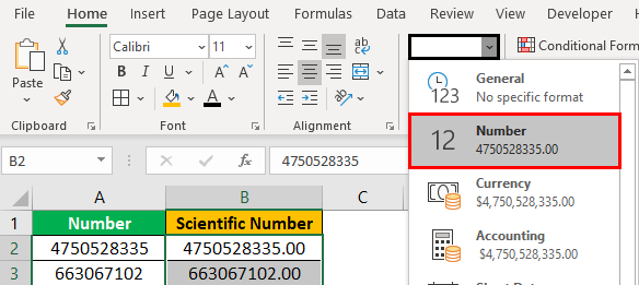
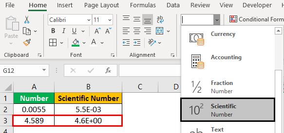
At the bottom, you can see the “Scientific” formatting option. Click on this to apply this formatting.

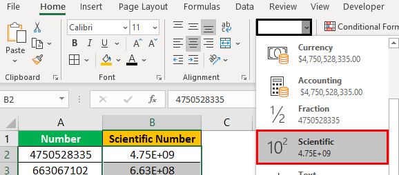
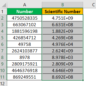
Now, scientific formatting is applied to large and small numbers.

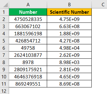
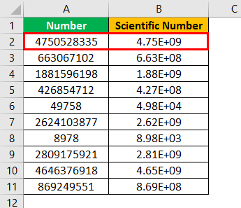
Now, take an example of the first instance. General formatting number was 4750528335 and scientific number is 4.75E+09 i.e. 4.75 x 109 (10 * 10 * 10 * 10 * 10 * 10 * 10 * 10 * 10).

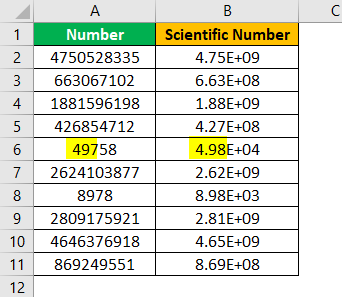
Now, look at A6 cell value, general formatting value was 49,758 and scientific value is 4.98E+04 i.e. 4.98 * 104 (10 * 10 * 10 * 10).

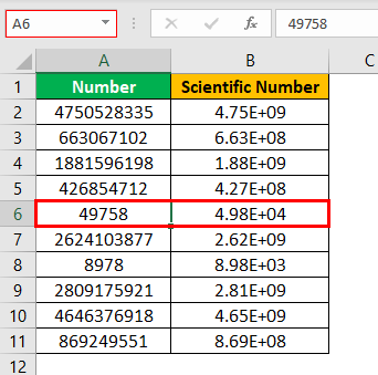
As you can see, the decimal value should have been 4.97. But, instead, it shows as 4.98. It is because after two digits of decimal third digit value are “5,” it is rounded to the nearest number. So, instead of 97, it will be 98.

If you do not want to see this rounding off to the nearest values, you can increase the decimal value from 2 to 3 digits.

Now, we can see scientific numbers in three digits.

Example #2 – For Negative Exponent

You need to know how negative exponent works with excelIn Excel, exponents are the same exponential function as in mathematics, where a number is raised to a power or exponent of another number. Exponents can be used by two methods: the power function or the exponent symbol on the keyboard.read more scientific notation. Now, look at the below image.

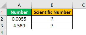
First value is 0.0055 which is formatted as 5.5E-03, 5.5 x 10-3.

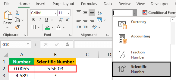
Now look at the second number 4.589, which is formatted as 4.6E+00, i.e., 4.6 x 10⁰

Things to Remember

We must first understand how scientific notation works in mathematics and then learn the same in excel.
We can only change the decimal values like 2, 3, and 4 digits.
Excel uses scientific format automatically for large and small numbers of 12-digit values or more.

How do you write 10 to the power of 3 in Excel?

The power of exponent in Excel is a carot symbol (SHIFT + 6 keyboard shortcut) which is ^. So you will write 10 to the 3rd power in Excel by 10^3. To type exponents in Excel just use carot. In cell you can just write =10^3.

How do I change e+ in Excel?

To remove scientific formatting from a number in Excel, select the cells that you wish to remove the scientific formatting. Right-click and then select “Format Cells” from the popup menu. When the Format Cells window appears, select the Number tab and highlight Number under the Category.

How do I get rid of E 21 in Excel?

Just right click on the cell and choose Format cell. Change the format from General to Number with zero number of decimal places.

How do I get rid of E 11 in Excel?

To get rid of e+, all you need to do is select the particular cell and change the format from General to Number…and you’re done! Select the cells that will hold the larger values and right-click the selection. Select Format Cells. In the Number tab, select the desired format (e.g., Number) and click OK.

How do you write 10 to the power 9 in Excel?

Use the “Power” function to specify an exponent using the format “Power(number,power).” When used by itself, you need to add an “=” sign at the beginning. As an example, “=Power(10,2)” raises 10 to the second power.

How do you convert scientific notation to decimal?

Convert scientific notation to decimal form

Determine the exponent, n , on the factor 10 .
Move the decimal n places, adding zeros if needed. If the exponent is positive, move the decimal point n places to the right. If the exponent is negative, move the decimal point |n| places to the left.
Check.

A number is written in scientific notation when a number between 1 and 10 is multiplied by a power of 10. For example, 650,000,000 can be written in scientific notation as 6.5 ✕ 10^8.

Why does Excel change my numbers to scientific notation?

The program is designed to cap numbers at 15 digits, in order to preserve accuracy. So, when you open up your CSV that contains 15+ digit numbers, Excel automatically converts that to scientific notation as a way of dealing with that limit.

How do you remove scientific notation from sheets?

Here’s what you have to do:

Open your spreadsheet.
Select the range of cells.
Click on Format.
Click on Number (or the “123” sign).
You’ll see that the “Scientific” option was selected.
Unselect it and select any other option.

How do you convert standard notation to scientific notation?

To change a number from scientific notation to standard form, move the decimal point to the left (if the exponent of ten is a negative number), or to the right (if the exponent is positive). You should move the point as many times as the exponent indicates.

What does e8 mean?

E-8 (rank), an enlisted rank in the military of the United States.

How do you stop scientific notation in CSV?

8 Answers

Open as an excel sheet (or convert if you can’t open as one)
highlight the (barcode/scientific notation) column.
Go into Data / text to columns.
Page 1: Check ‘Delimited’ / Next.
Page 2: Check ‘ Tab’ and change ‘Text Qualifier’ to ” / Next.
Page 3: Check ‘Text’ rather than ‘general’
Finish.

How do you convert scientific notation to date in Excel?

How to format cells in Excel

Press Ctrl + 1 shortcut.
Right click the cell (or press Shift+F10), and select Format Cells… from the pop-up menu.
Click the Dialog Box Launcher arrow at the bottom right corner of the Number, Alignment or Font group to open the corresponding tab of the Format Cells dialog:

How do I fix e 12 in Excel?

Method 1: Format the cell as text

Right-click target cell, and then click Format Cells.
On the Number tab, select Text, and then click OK.
Then type a long number. (
If you do not want to see the warning arrows, click the small arrow, and then click Ignore Error.

What is E 05 Excel?

2.3e-5, means 2.3 times ten to the minus five power, or 0.000023. 4.5e6 means 4.5 times ten to the sixth power, or 4500000 which is the same as 4,500,000.

How do you do exponential in Excel?

How to Use Exponents in Excel

Exponents are simply repeated multiplications.
Under “Category:” on the left, select “Text,” and then click “OK.”
In the same cell, type both the base number and exponent without any spaces between them.
Next, highlight your exponent; in our example, it’s the three.

How do you write 4th in Excel?

Keyboard shortcuts for superscript and subscript in Excel

Select one or more characters you want to format.
Press Ctrl + 1 to open the Format Cells dialog box.
Then press either Alt + E to select the Superscript option or Alt + B to select Subscript.
Hit the Enter key to apply the formatting and close the dialog.

How do I write cm2 in Excel?

Follow these steps:

Click inside a cell on your worksheet.
Type =N^2 into the cell, where N is the number you want to square. For example, to insert the square of 5 into cell A1, type =5^2 into the cell.
Press Enter to see the result. Tip: You can also click into another cell to see the squared result.

How do you write 245000 in scientific notation?

245,000 (two hundred forty-five thousand) is an even six-digits composite number following 244999 and preceding 245001. In scientific notation, it is written as 2.45 × 10⁵.

How do you write 1.5 in scientific notation?

The number 10 is called the base because it is this number that is raised to the power n. Although a base number may have values other than 10, the base number in scientific notation is always 10.
1.5: Scientific Notation – Writing Large and Small Numbers.

	Explanation	Answer
d	Because the decimal point was moved four places to the left, n = 4.	1.2378×104

Источник

In this post, you’ll learn how to display numbers in Excel using engineering notation, how engineering notation differs from scientific notation, and how custom formats work in Excel

[toc]

Video

Subscribe to EngineerExcel on YouTube

Numbers can be displayed in Excel using engineering notation by creating the following custom format:

##0.0E+0

For more information about displaying numbers in engineering notation in Excel, continue reading:

Engineering Notation Background

Engineering notation is a way of expressing either very large or very small numbers in a readable way using exponential notation.

Engineering notation allows us to quickly determine whether the prefix on a unit is milli-, micro-, nano-, kilo-, mega-, giga-, or so on.

Scientific notation also provides a way of displaying very small and very large numbers, but it’s not as convenient because the exponent can be any integer.

By default, Excel can display values using scientific notation, but it does not have an engineering notation format built in. However, we can use a custom number format to display numbers this way.

Worksheet Inputs

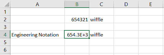
To start, I’ll enter a number into the spreadsheet in cell B2. Just for fun, let’s just give it the unit of wiffles (believe it or not, this is a legitimate unit of measurement).

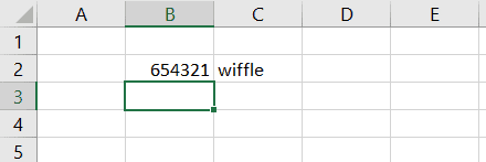
Worksheet Outputs

In cell B4, we’ll display the number in engineering notation. So, I’ll set cell B4 equal to cell B2.

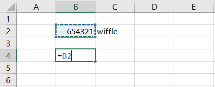
How to Display Engineering Notation in Excel

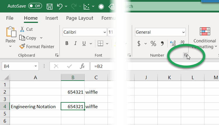
Next, let’s create the custom format for cell B4 to show the value in engineering notation.

To do that, select B4 and click the icon at the lower right of the Number group in the Home tab of Excel ribbon.

Custom Format for Engineering Notation

In the number tab, select Custom.

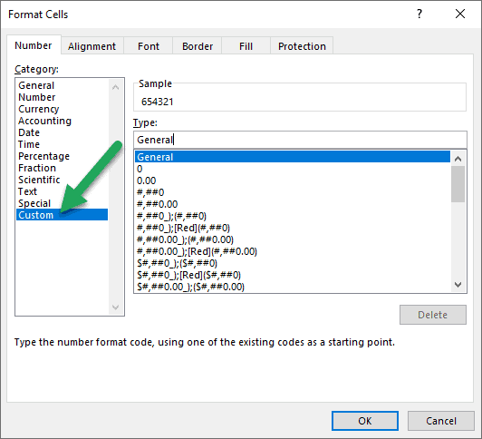
And then in the “Type” field, enter the symbols to create the custom format:

##0.0E+0

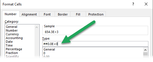
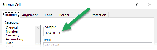
We can see a preview of how the number in the cell will look in the Sample field at the top of the window.

Click OK.

The value in cell B4 is in engineering notation because 10 (represented by the letter E) is raised to the power of a number that is a multiple of three. In this case, it’s exactly three. So, there are 654.3 kilowiffles.

Engineering Notation vs. Scientific Notation in Excel

Let’s compare that to how the number would be displayed in scientific notation.

Set cell B6 equal the cell B2 and select cell B6.

Then, from the number group in the home ribbon, select the scientific format.

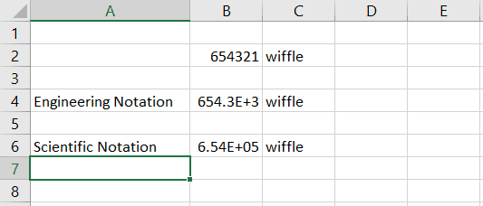
Scientific notation is very similar, but there’s one key distinction. The exponent is not a multiple of three, which makes it difficult to understand the prefix on the units.

How Engineering Notation Responds to Changes in the Magnitude of a Cell Value

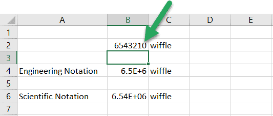
When we increase the order of magnitude of the input value in cell B2, the value in cell B4 changes to 6.5E+6 or 6.5 times 10 raised to the power of six. Six is a multiple of three, so this is still engineering notation. And because we’re using engineering notation, it’s easy to tell that now we are talking about 6.5 mega-wiffles.

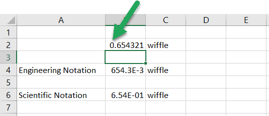
This engineering notation works, even when we’re talking about numbers that are less than zero. If a decimal point is added to the beginning of the number in cell B2, now we have 654.3 milli-wiffles.

How the Excel Custom Format for Engineering Notation Works

Let’s take a closer look at the custom number format we created to understand how engineering notation works in Excel.

The “#”and “0” placeholders in the custom format each do specific things.

Whenever there is a zero in a custom format, a digit will be displayed there, even if it is an insignificant zero. With this format, there will always be a digit directly to the right and left of the decimal point because there are zeroes on either side of the decimal point.

The “#” sign is essentially an optional placeholder. It will not display insignificant zeros and will only display a digit when there is one to be displayed.

The combination of two #’s and a 0 on the left side of the decimal point forces Excel to display between one and three digits to the left of the decimal point. This will yield a number between zero and 999 on the left side. If the number is 1000, it will be displayed as 1.0E+3.

In this format, there will always be one digit displayed to the right of the decimal point. We can increase that by adding more zeros to the right of the decimal point.

Источник

Need more help?

Want more options?

How to format the cell to disable scientific notation?

Increasing the number of decimal places

Using the Custom format

Using the ROUND formula

How to concatenate the cell to disable scientific notation?

Conversion of the cell to disable scientific notation

Trimming to remove scientific notation

Using the IF function

Using the FIX function

Using the INT function

Using the TRUNC function

Pasting values as text

Table of contents

How to Format Scientific Notation in Excel? (with Examples)

Example #1 – For Positive Exponent

Example #2 – For Negative Exponent

Things to Remember

Recommended Articles

How do you write 10 to the power of 3 in Excel?

How do I change e+ in Excel?

How do I get rid of E 21 in Excel?

How do I get rid of E 11 in Excel?

How do you write 10 to the power 9 in Excel?

How do you convert scientific notation to decimal?

Why does Excel change my numbers to scientific notation?

How do you remove scientific notation from sheets?

How do you convert standard notation to scientific notation?

What does e8 mean?

How do you stop scientific notation in CSV?

How do you convert scientific notation to date in Excel?

How do I fix e 12 in Excel?

What is E 05 Excel?

How do you do exponential in Excel?

How do you write 4th in Excel?

How do I write cm2 in Excel?

How do you write 245000 in scientific notation?

How do you write 1.5 in scientific notation?

Contents

Video

Engineering Notation Background

Worksheet Inputs

Worksheet Outputs

How to Display Engineering Notation in Excel

Custom Format for Engineering Notation

Engineering Notation vs. Scientific Notation in Excel

How Engineering Notation Responds to Changes in the Magnitude of a Cell Value

How the Excel Custom Format for Engineering Notation Works