
Excel for Microsoft 365 Excel for Microsoft 365 for Mac Excel for the web Excel 2021 Excel 2021 for Mac Excel 2019 Excel 2019 for Mac Excel 2016 Excel 2016 for Mac Excel 2013 Excel 2010 Excel 2007 Excel for Mac 2011 Excel Starter 2010 More…Less
This article describes the formula syntax and usage of the TRIM function in Microsoft Excel.
Description
Removes all spaces from text except for single spaces between words. Use TRIM on text that you have received from another application that may have irregular spacing.
Important: The TRIM function was designed to trim the 7-bit ASCII space character (value 32) from text. In the Unicode character set, there is an additional space character called the nonbreaking space character that has a decimal value of 160. This character is commonly used in Web pages as the HTML entity, . By itself, the TRIM function does not remove this nonbreaking space character. For an example of how to trim both space characters from text, see Top ten ways to clean your data.
Syntax
TRIM(text)
The TRIM function syntax has the following arguments:
-
Text Required. The text from which you want spaces removed.
Example
Copy the example data in the following table, and paste it in cell A1 of a new Excel worksheet. For formulas to show results, select them, press F2, and then press Enter. If you need to, you can adjust the column widths to see all the data.
|
Formula |
Description |
Result |
|
=TRIM(» First Quarter Earnings «) |
Removes leading and trailing spaces from the text in the formula (First Quarter Earnings) |
First Quarter Earnings |
Need more help?
Want more options?
Explore subscription benefits, browse training courses, learn how to secure your device, and more.
Communities help you ask and answer questions, give feedback, and hear from experts with rich knowledge.
Skip to content
Вы узнаете несколько быстрых и простых способов, чтобы удалить начальные, конечные и лишние пробелы между словами, а также почему функция Excel СЖПРОБЕЛЫ (TRIM в английской версии) не работает и как это исправить.
Вы сравниваете два столбца на предмет наличия дубликатов, но ваши формулы не могут найти ни одной повторяющейся записи? Или вы складываете два столбца чисел, но получаете только нули? И почему, черт возьми, ваша очевидно правильная формула ВПР возвращает только кучу ошибок Н/Д? Это лишь несколько примеров проблем, на которые вы, возможно, ищете ответы. И все это вызвано дополнительными пробелами, скрытыми до, после или между числовыми и текстовыми значениями в ваших ячейках.
- Как удалить лишние пробелы в столбце?
- Удаление ведущих пробелов
- Как сосчитать лишние пробелы?
- Выделение цветом ячеек с лишними пробелами
- А если СЖПРОБЕЛЫ не работает?
- Инструмент Trim Spaces — удаляйте лишние пробелы одним щелчком мыши.

Microsoft Excel предлагает несколько различных способов очистки данных. В этом руководстве мы исследуем возможности функции СЖПРОБЕЛЫ как самого быстрого и простого способа удаления пробелов в Excel.
Итак, функция СЖПРОБЕЛЫ в Excel применяется, чтобы удалить лишние интервалы из текста. Она удаляет все начальные, конечные и промежуточные, за исключением одного пробела между словами.
Синтаксис её самый простой из возможных:
СЖПРОБЕЛЫ(текст)
Где текст — это ячейка, из которой вы хотите удалить лишние интервалы (или просто текстовая строка, заключённая в двойные кавычки).
Например, чтобы удалить их в ячейке A1, используйте эту формулу:
=СЖПРОБЕЛЫ(A1)
И это скриншот показывает результат:

Ага, это так просто!
Если в дополнение к лишним пробелам ваши данные содержат разрывы строк и непечатаемые символы, используйте функцию СЖПРОБЕЛЫ в сочетании с ПЕЧСИМВ (CLEAN в английской версии), чтобы удалить первые 32 непечатаемых символа в кодовой системе ASCII.
Например, чтобы удалить пробелы, разрывы строк и другие нежелательные символы из ячейки A1, используйте эту формулу:
=СЖПРОБЕЛЫ(ПЕЧСИМВ(A1))
Дополнительные сведения см. В разделе Как удалить непечатаемые символы в Excel.
Теперь, когда вы знаете основы, давайте обсудим несколько примеров использования СЖПРОБЕЛЫ в Excel, а также те подводные камни, с которыми вы можете столкнуться.
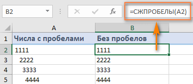
Как убрать лишние пробелы во всём столбце.
Предположим, у вас есть столбец с именами, в котором есть пробелы до и после текста, а также более одного интервала между словами. Итак, как удалить все начальные, конечные и лишние промежуточные пробелы во всех ячейках одним махом?
Записав формулу Excel СЖПРОБЕЛЫ в соседний столбец, а затем заменив формулы их значениями. Подробные инструкции приведены ниже.
Напишите это выражение для самой верхней ячейки, A2 в нашем примере:
=СЖПРОБЕЛЫ(A2)
Поместите курсор в нижний правый угол ячейки формулы (B2 в этом примере), и как только курсор превратится в знак плюса, дважды щелкните его, чтобы скопировать вниз по столбцу, до последней ячейки с данными. В результате у вас будет 2 столбца — исходные имена с интервалами и имена, приведённые в порядок при помощи формулы.

Наконец, замените значения в исходном столбце новыми данными. Но будьте осторожны! Простое копирование нового столбца поверх исходного сломает ваши формулы. Чтобы этого не случилось, нужно копировать только значения, а не ячейки целиком.
Вот как это сделать:
Выделите все ячейки с расчетами (B2:B8 в этом примере) и нажмите Ctrl + C, чтобы скопировать их. Или по правой кнопке мыши воспользуйтесь контекстным меню.
Выделите все ячейки со старыми данными (A2:A8) и нажмите Ctrl + Alt + V. Эта комбинация клавиш вставляет только значения и делает то же самое, что и контекстное меню Специальная вставка > Значения.
Нажмите ОК. Готово!
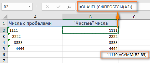
Как удалить ведущие пробелы в числовом столбце
Как вы только что видели, функция Excel СЖПРОБЕЛЫ без проблем удалила все лишние интервалы из столбца текстовых данных. Но что, если ваши данные — числа, а не текст?
На первый взгляд может показаться, что функция СЖПРОБЕЛЫ сделала свое дело. Однако при более внимательном рассмотрении вы заметите, что обрезанные значения не ведут себя как числа. Вот лишь несколько признаков аномалии:
- И исходный столбец, и обрезанные числа выравниваются по левому краю, даже если вы применяете к ним числовой формат. В то время как обычные числа по умолчанию выравниваются по правому краю.
- Когда выбраны две или более ячеек с очищенными числами, Excel отображает только КОЛИЧЕСТВО в строке состояния.Для чисел он также должен отображать СУММУ и СРЕДНЕЕ.
- Формула СУММ, примененная к этим ячейкам, возвращает ноль.
И что нам с этим делать?
Небольшой лайфхак. Если вы вместо СЖПРОБЕЛЫ(A2) используете операцию умножения на 1, то есть A1*1, то получите тот же результат. И еще один элегантный способ избавления от пробелов перед числом:
=—A1
Но обращаю внимание, что результатом будет являться по-прежнему текст.
А вот такое хитрое выражение сразу превратит текст “ 333” в число 333:
=—(—A1)
Вы видите, что все цифры выровнены по левому краю. Дело в том, что очищенные значения представляют собой текстовые строки, а нам нужны числа. Чтобы исправить это, вы можете умножить «обрезанные» значения на 1 (чтобы умножить все значения одним махом, используйте опцию Специальная вставка > Умножить).
Более элегантное решение — заключить функцию СЖПРОБЕЛЫ в ЗНАЧЕН, например:
=ЗНАЧЕН(СЖПРОБЕЛЫ(A2))
Приведенное выше выражение удаляет все начальные и конечные пробелы, если они есть, и превращает полученное значение в число, как показано на скриншоте ниже:
И более того, если вам нужно именно число, то можете вовсе не утруждать себя удалением лишних символов перед цифрами. Выражение
=ЗНАЧЕН(A2)
сделает это за вас, и вы сразу получите на выходе число, с которым можно производить различные математические операции.
Кроме того, вы можете применить функцию Excel СЖПРОБЕЛЫ для удаления только начальных пробелов, сохраняя их все в середине текстовой строки без изменений. Пример формулы здесь: Как удалить только ведущие пробелы?
Как посчитать лишние пробелы в ячейке.
Чтобы получить количество лишних пробелов в ячейке, узнайте общую длину текста с помощью функции ДЛСТР, затем вычислите длину строки без дополнительных интервалов и вычтите последнее из первого:
=ДЛСТР(A2)-ДЛСТР(СЖПРОБЕЛЫ(A2))
На рисунке ниже показана приведенная выше формула в действии:
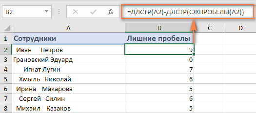
Примечание. Выражение возвращает количество дополнительных пробелов в ячейке, т.е. ведущих, конечных и более одного последовательного интервала между словами, но не учитывает отдельные пробелы в середине текста. Если вы хотите получить общее количество пробелов в ячейке, используйте эту формулу замены.
Как выделить ячейки с лишними пробелами?
При работе с конфиденциальной или важной информацией вы можете не решаться удалить что-либо, не видя, что именно вы удаляете. В этом случае вы можете сначала выделить ячейки, содержащие лишние пробелы, а затем безопасно удалить их.
Для этого создайте правило условного форматирования со следующей формулой:
=ДЛСТР($A2)>ДЛСТР(СЖПРОБЕЛЫ($A2))
Где A2 – самый верхний адрес с данными, которые вы хотите выделить.
Мы указываем Excel выделять ячейки, в которых общая длина строки больше, чем длина обрезанного текста.
Чтобы создать правило условного форматирования, выберите все ячейки, которые вы хотите выделить, без заголовков столбцов, перейдите на вкладку «Главная » и нажмите « Условное форматирование» > «Новое правило» > «Используйте формулу…».
Если вы еще не знакомы с условным форматированием Excel, вы найдете подробные инструкции здесь: Как создать правило условного форматирования на основе формулы .
Как показано на скриншоте ниже, результат полностью подтверждается числами, которые мы получили в соседнем столбце:

Как видите, использовать функцию СЖПРОБЕЛЫ в Excel довольно просто.
Если не работает …
Функция СЖПРОБЕЛЫ предназначена для удаления только символа пробела, представленного значением кода 32 в 7-битном наборе символов ASCII. В наборе Unicode есть так называемый неразрывный пробел, который обычно используется на веб-страницах как символ html & nbsp; . Он имеет десятичное значение 160, и функция СЖПРОБЕЛЫ не может удалить его сама. При копировании текста с веб-страниц или из Word вы вполне можете получить его в свою таблицу.
Иногда такие неразрывные пробелы вставляют специально, чтобы фраза в ячейке не разделялась по строкам. К примеру, некрасиво будет, если инициалы будут оторваны от фамилии и перенесены на следующую строку. В Microsoft Word такой спецсимвол вводится сочетанием клавиш Ctrl+Shift+Пробел.
Итак, если ваш набор данных содержит один или несколько пробелов, которые нашими стандартными методами не получается убрать, используйте функцию ПОДСТАВИТЬ, чтобы преобразовать неразрывные пробелы в обычные, а затем избавиться от их. Предполагая, что текст находится в A1, выражение выглядит следующим образом:
=СЖПРОБЕЛЫ(ПОДСТАВИТЬ(A2; СИМВОЛ(160); » «))
В качестве дополнительной меры предосторожности вы можете встроить функцию ПЕЧСИМВ для очистки ячейки от любых непечатаемых символов:
=СЖПРОБЕЛЫ(ПЕЧСИМВ(ПОДСТАВИТЬ(A2; СИМВОЛ(160); » «)))
На этом рисунке показана разница:

Если приведенные выше варианты также не работают, скорее всего, ваши данные содержат некоторые определенные непечатаемые символы с кодовыми значениями, отличными от 32 и 160.
В этом случае используйте одну из следующих формул, чтобы узнать код символа, где A1 — проблемная ячейка:
Перед текстом: = КОДСИМВ (ЛЕВСИМВ(A1;1))
После текста: = КОДСИМВ (ПРАВСИМВ(A1;1))
Внутри ячейки (где n — позиция проблемного знака в текстовой строке):
=КОДСИМВ(ПСТР(A1; n; 1)))
Затем передайте найденный код проблемного символа в СЖПРОБЕЛЫ(ПОДСТАВИТЬ()), как описано выше.
Например, если функция КОДСИМВ возвращает 9, что является знаком горизонтальной табуляции, используйте следующую формулу для ее удаления:
=СЖПРОБЕЛЫ(ПОДСТАВИТЬ(A2; СИМВОЛ(9); » «))
Инструмент Trim Spaces — удаляйте лишние пробелы одним щелчком мыши.
Если применение формул представляет сложность для вас, тогда вам может понравиться этот метод буквально в один клик, чтобы избавиться от пробелов в Excel. Надстройка Ultimate Suite среди множества полезных инструментов, например, изменение регистра, разделение текста и извлечение из него нужных символов, предлагает опцию «Удалить пробелы» .
Если в Excel установлен Ultimate Suite, то удалить пробелы будет очень просто:
- Выберите одну или несколько ячеек, в которой вы хотите убрать пробелы.
- Нажмите кнопку «Trim Spaces» на ленте.
- Выберите один, несколько или сразу все из следующих вариантов:
- Обрезать начальные и конечные пробелы.
- Удалить лишние пробелы между словами, кроме одного.
- Удалить неразрывные пробелы ( )
- Удалить лишние переносы строк до и после значений, между значениями оставить только один.
- Удалить все переносы строк в ячейке.
- Нажмите кнопку Обрезать (Trim).
Вот и все! Все лишние пробелы удаляются в мгновение ока.
В этом примере мы удаляем всё лишнее, сохраняя только по одному пробелу между словами.

Задача, с которой не справляются формулы Excel, выполняется одним щелчком мыши! Вот результат:

А вот обзор других возможностей работы с текстовыми данными — изменить регистр символов, добавить текст в начале в конце, перед или после выбранных символов, удалить непечатаемые символы, извлечь часть текста по позиции или после указанных символов, извлечь числа из текста, разделить текст по столбцам или строкам и другие полезные операции.
Если вы хотите попробовать этот инструмент на своих данных, вы можете загрузить ознакомительную версию.
Благодарю вас за чтение и с нетерпением жду встречи с вами. В нашем следующем уроке мы обсудим другие способы удаления пробелов в Excel, следите за обновлениями!
 Формула ЗАМЕНИТЬ и ПОДСТАВИТЬ для текста и чисел — В статье объясняется на примерах как работают функции Excel ЗАМЕНИТЬ (REPLACE в английской версии) и ПОДСТАВИТЬ (SUBSTITUTE по-английски). Мы покажем, как использовать функцию ЗАМЕНИТЬ с текстом, числами и датами, а также…
  Как быстро посчитать количество слов в Excel — В статье объясняется, как подсчитывать слова в Excel с помощью функции ДЛСТР в сочетании с другими функциями Excel, а также приводятся формулы для подсчета общего количества или конкретных слов в…
  Как быстро извлечь число из текста в Excel — В этом кратком руководстве показано, как можно быстро извлекать число из различных текстовых выражений в Excel с помощью формул или специального инструмента «Извлечь». Проблема выделения числа из текста возникает достаточно…
  Как убрать пробелы в числах в Excel — Представляем 4 быстрых способа удалить лишние пробелы между цифрами в ячейках Excel. Вы можете использовать формулы, инструмент «Найти и заменить» или попробовать изменить формат ячейки. Когда вы вставляете данные из…
  Как удалить пробелы в ячейках Excel — Вы узнаете, как с помощью формул удалять начальные и конечные пробелы в ячейке, лишние интервалы между словами, избавляться от неразрывных пробелов и непечатаемых символов. В чем самая большая проблема с…
  Функция ПРАВСИМВ в Excel — примеры и советы. — В последних нескольких статьях мы обсуждали различные текстовые функции. Сегодня наше внимание сосредоточено на ПРАВСИМВ (RIGHT в английской версии), которая предназначена для возврата указанного количества символов из крайней правой части…
  Функция ЛЕВСИМВ в Excel. Примеры использования и советы. — В руководстве показано, как использовать функцию ЛЕВСИМВ (LEFT) в Excel, чтобы получить подстроку из начала текстовой строки, извлечь текст перед определенным символом, заставить формулу возвращать число и многое другое. Среди…
Bottom Line: Learn 5 different techniques to find and remove spaces in Excel. Spaces can cause formula errors and frustration with data preparation and analysis.
Skill Level: Intermediate
Watch the Tutorial
Download the Excel File
You can download the workbook that I use in the video, including the macro I wrote to remove blank spaces.
Space Hunting
Blank spaces can be a headache for data analysts and formula writers. That’s because they are not easy to spot, yet can cause frustrating calculation errors.
After many years of working with Excel, I’ve become a Space Hunter. That sounds like a sci-fi movie title, but it’s just someone who can quickly locate and delete superfluous spaces in cell values.
Based on my space hunting experience, here are five techniques I use frequently to clean up data.
1. Find & Replace
The first method for space hunting is to use the Find & Replace feature.
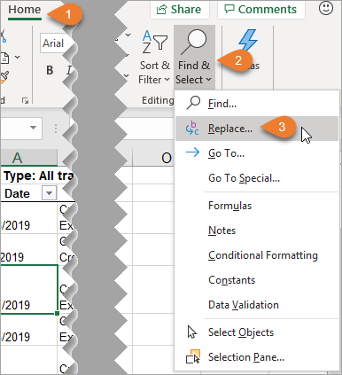
After highlighting the cells that you want to search through, go to the Home tab. Then open the Find & Select dropdown menu. Select the Replace option. The keyboard shortcut for this is Ctrl + H.
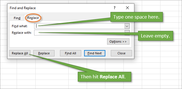
That will bring up the Find and Replace window. On the Replace tab, place one blank space in the Find what field. Make sure there is nothing in the Replace with field. Hitting Replace All (keyboard shortcut: Alt+A) will remove any instances of a space in the data set that you selected.
Although this method is really quick and easy, it’s only useful for data where you want ALL spaces removed. However, there are times when you want to keep spaces between words. For example, if your cells contain both first and last names, you will probably want to keep the space in between those names.
That scenario leads us to our second method for space hunting.
2. The TRIM Function
The TRIM function removes all spaces in a text string, except for single spaces between words.
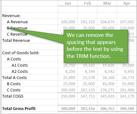
Below is an example of a report where some of the cells look like they are indented but the indentation is actually just extra spaces. Let’s say we want to remove those spaces for uniformity’s sake. We can use the TRIM function to do that.
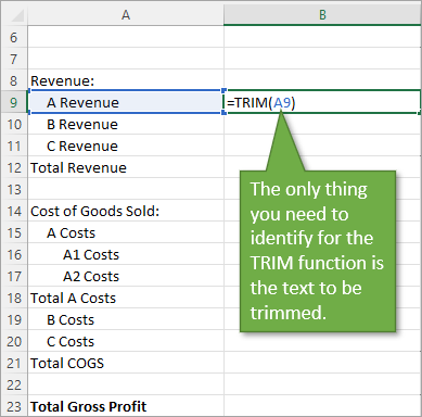
In a blank column, start by typing the equals sign (=) and the word TRIM, then tab into the TRIM function.
The only thing you need to identify for the TRIM function to work is the text that needs trimming. So either type the name of the cell or click on the cell that you want to trim and hit Enter. This will return the result you’re looking for: text with no spaces before or after it.
When you copy the formula down for the whole column, the result looks like this.
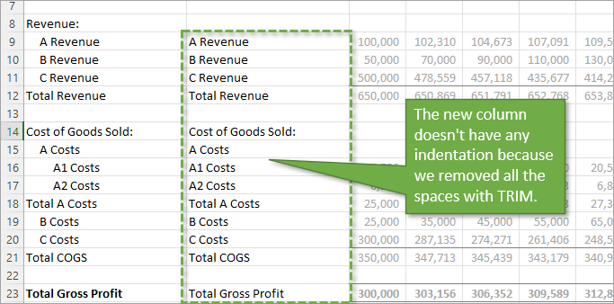
As you can see, the spacing between the words remains in place, but any spacing before or after the text is removed.
With this method, we had to create a whole new column, so you would have to add the additional step of replacing the original column with the new one using Copy and Paste Values. You can then delete the column with the formulas.
3. Power Query
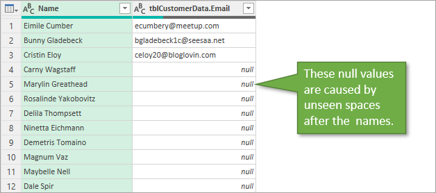
Like functions and formulas, queries can also be tripped up by the inclusion of a stray blank space.
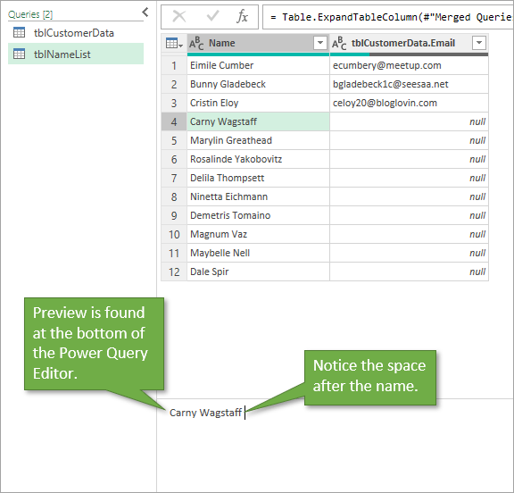
If you are unsure if blank spaces are what’s causing the problem, you can click into the Editor’s preview to see if there is a space or not.
To remove the spaces, Power Query has a Trim feature found in the right-click menu. With the column that you want to fix selected, just right-click and choose Transform, and Trim.
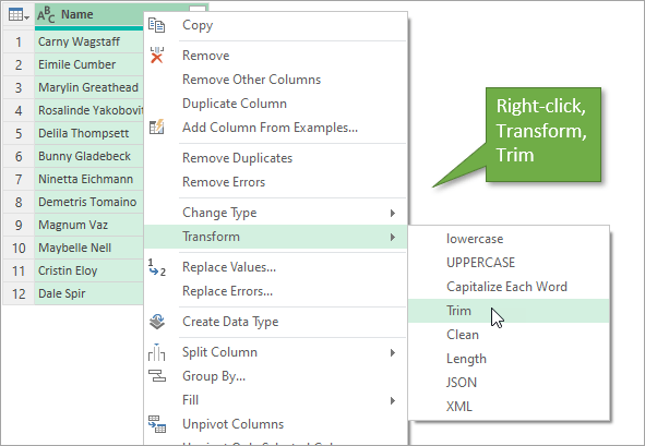
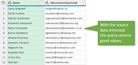
This trims all the blank space before/after the text string so that the query will return the correct values.
If you are relatively new to Power Query, or could use a refresher, I recommend checking out my free webinar: The Modern Excel Blueprint.

4. Macros and VBA
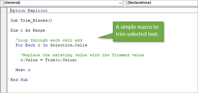
Let’s look at the same example we used for the TRIM function, but this time we will use a macro to trim extra spaces from text.
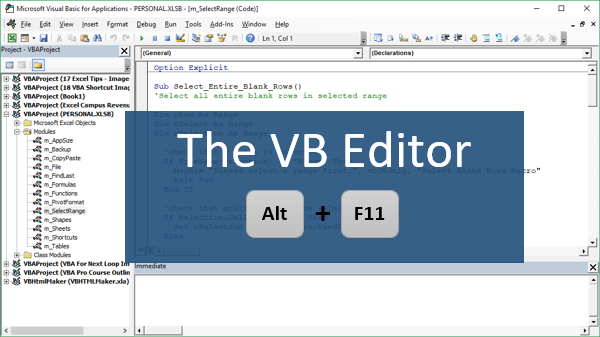
Start by opening the VB Editor. Go to the Developer tab and select the Visual Basic Button. The keyboard shortcut is Alt + F11.
I’ve written a simple macro that loops through each cell and replaces the value of the cell with the trimmed value. If you’d like to copy this macro, you can find it in the download file at the top of this post.
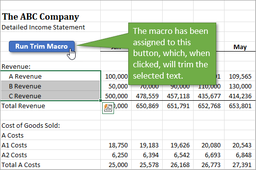
One of the benefits of using a macro is that you can assign it to a button. Here I’ve assigned it to a button on the actual worksheet.
And here, I’ve added it to the ribbon by including this macro in my Personal Macro Workbook and assigning a button to it.
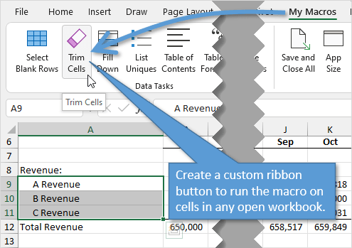
That way, I can use this macro on any workbook.
One downside to using the macro method for removing blank spaces is that you cannot undo the action once the macro has been run. In that case, it might be a good idea to save the file before running the macro, if you think you might need to un-trim the data for some reason.
It’s also important to note that the VBA Trim function does NOT trim extra blank spaces between words. Excel’s TRIM function will remove additional spaces between words. So if there are two spaces between the first and last name, TRIM will remove the additional space. VBA’s Trim will not do this. It only removes spaces from the beginning or end of the string. Thanks to Marvin (an Excel Campus Community Member) for bringing this to our attention!
Here are tutorials for how to create a Personal Macro Workbook as well as how to make Macro buttons, whether on the worksheet or in the ribbon.
How to Create a Personal Macro Workbook (Video Series)
How to Create Macro Buttons in Excel Worksheets
5. Trimming Other Characters
Sometimes after you have trimmed the spaces from your text, you might still get calculation errors. One reason for this could be that another hard-to-detect character might be in play. One such character is the non-breaking space. This is often used in HTML coding ( ) and is similar to a regular space, but would not be deleted by the TRIM function or our macro.
To determine which character might be gumming up the works, you can use the CODE function. By copying and pasting the invisible character into a blank cell, and then identifying that cell’s text in the CODE function (“text” is the only argument that needs to be identified for the CODE function), you will return a code number for that character. A quick Google search of that code number will reveal what type of character you are dealing with.
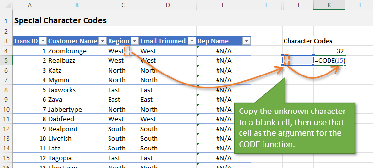
In this case, the non-breaking space character is code 160.
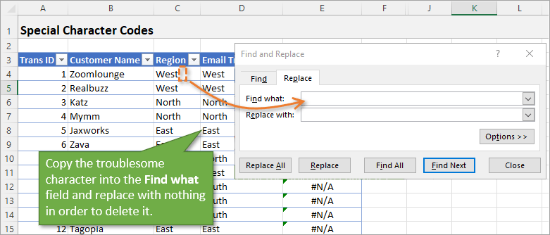
One way to remove that character from your text would be to use Find & Replace. You can simply copy the character and paste it into the Find what field.
You could also use the REPLACE function to do the same thing.
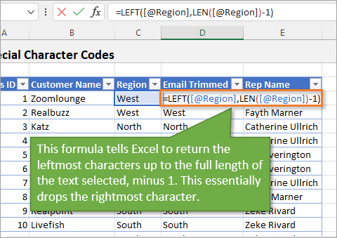
One other option, since we know we want to remove the last character in the text, would be to use the LEFT and LEN functions to essentially create a customized trim feature.
LEFT returns the leftmost characters in a cell, up to a designated amount. LEN (short for Length) returns the number of characters in a cell.
So combining those two functions and subtracting 1 from the LEN to remove that unwanted character would leave just the text without the additional character.
Conclusion
I hope this has been helpful for you. I also explain how spaces can cause errors in formulas in my video on an Introduction to VLOOKUP.
There are actually more than just five ways to go about this task, and if you’d like to add to the list, please leave a comment below. As always, you can ask questions there as well.
Thanks for following along. Until next time!
Watch Video – Remove Spaces in Excel
Leading and trailing spaces in Excel often leads to a lot of frustration. I can’t think of a situation where you may need these extra spaces, but it often finds its way into the excel spreadsheets.
There are many ways you can end up with these extra spaces – for example, as a part of the data download from a database, while copying data from a text document, or entered manually by mistake.
Leading, trailing, or double space between text could lead to a lot of serious issues.
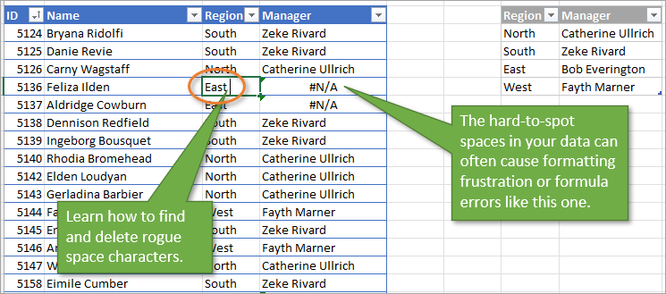
For example, suppose you have a data set as shown below:

Now have a look at what happens when I use a VLOOKUP function to get the last name using the first name.

You might not be able to spot the difference with the naked eye that there is an extra trailing space in the name that is causing this error.

In this example, it was easy to spot the issue in such a small data set, but imagine having to check this for thousands of records.
To be on the safe side, it is always a good idea to clean your data and remove spaces in Excel.
How to Remove Spaces in Excel
In this tutorial, I will show you two ways to remove spaces in Excel.
- Using TRIM function.
- Using Find and Replace.
Using the TRIM Function
Excel TRIM function removes the leading and trailing spaces, and double spaces between text strings.
For example, in the above example, to remove spaces from the entire list if first names (in A2:A7), use the following formula in cell C1 and drag it down for all the first names:
=TRIM(A2)
Excel TRIM function would instantly remove all the leading and trailing spaces in the cell.
Once you have the cleaned data, copy it paste it as values in place of the original data.
This function is also helpful if you have more than one space character between words. It would remove the extra spaces such that the result always have one space character between words.
Excel TRIM function does a good job in removing spaces in Excel, however, it fails when you have non-printing characters (such as line breaks) in your data set. To remove non-printing characters, you can use a combination of TRIM and CLEAN functions.
If you have some text in cell A1 from which you want to remove spaces, use the below formula:
=TRIM(CLEAN(A1))
Non-printing characters can also result from =CHAR(160), which can not be removed by the CLEAN formula. So, if you want to be absolutely sure that you have all the extra spaces and non-printing characters, use the below formula:
=TRIM(CLEAN(SUBSTITUTE(A1,CHAR(160)," ")))
Remove Extra Spaces in Excel using FIND and REPLACE
You can remove spaces in Excel using the Find and Replace functionality.
This is a faster technique and can be useful in the given situations:
- When you want to remove double spaces.
- When you want to remove all the space characters.
Removing Double Spaces
Note that this technique cannot be used to remove leading or trailing spaces. It will find and replace double spaces irrespective of its position.
Here are the steps to do this:
This will replace all the double spaces with a single space character.

Note that this will only remove double spaces. If you have three space characters in between 2 words, it would result in 2 space characters (would remove one). In such cases, you can do this again to remove and any double spaces that might have been left.
Removing Single Spaces
To remove all the space characters in a data set, follow the below steps:
This will remove all the space characters in the selected data set.

Note that in this case, even if there are more than one space characters between two text strings or numbers, all of it would be removed.
Remove Line Breaks
You can also use Find and Replace to quickly remove line breaks.
Here are the steps to do this:
- Select the data.
- Go to Home –> Find and Select –> Replace (Keyboard Shortcut – Control + H).
- In the Find and Replace Dialogue Box:
- Find What: Press Control + J (you may not see anything except for a blinking dot).
- Replace With: Leave it empty.

- Replace All.

This will instantly remove all the line breaks from the data set that you selected.
Based on your situation, you can choose either method (formula or find and replace) to remove spaces in Excel.
You may also like the following Excel tutorials:
- Find and Remove Duplicates in Excel.
- 10 Super Neat Ways to Clean Data in Excel.
- MS Help – Remove Space and Non-printing characters.
- How to Remove the First Character from a String in Excel
- How to Remove Time from Date in Excel
Remove Spaces in Excel
While importing or copy-pasting the data from an external source, extra spaces are also copied in Excel. This makes the data disorganized and difficult to be used. The purpose of removing unwanted spaces from the excel data is to make it more presentable and readable for the user.
For example, if a cell contains “ rose,” the leading spaces may be visible to the reader. However, if “rose ” is written in a cell, the two trailing spaces may not be easily caught by the user.
Since extra spaces may render the Excel formulas incorrect, it is essential to eliminate them.
Table of contents
- Remove Spaces in Excel
- Top 5 Methods to Remove Spaces in Excel
- #1 – TRIM Function
- #2 – “Delimited” Option of Text to Columns Wizard
- #3 – “Fixed Width” Option of Text to Columns Wizard
- #4 – Find and Replace Option
- #5 – SUBSTITUTE Function
- Frequently Asked Questions
- Recommended Articles
Top 5 Methods to Remove Spaces in Excel
The five methods to remove extra spaces in Excel are listed as follows:
- TRIM function
- “Delimited” option of text to columns wizard
- “Fixed width” option of text to columns wizard
- Find and replace option
- SUBSTITUTE function
The user can select any of the techniques depending on the requirement. Let us discuss all the methods one by one, along with examples.
You can download this Remove Spaces Excel Template here – Remove Spaces Excel Template
#1 – TRIM Function
The TRIM functionThe Trim function in Excel does exactly what its name implies: it trims some part of any string. The function of this formula is to remove any space in a given string. It does not remove a single space between two words, but it does remove any other unwanted spaces.read more removes all spaces from a text string except for the single space between the words.
The following data contains extra spaces in column A. We want to rewrite the data without these spaces in column B with the help of the TRIM function.

Step 1: In cell B1, enter the TRIM function.

Step 2: Select the cell A1.

Step 3: Press the “Enter” key. The extra spaces from the name are removed in cell B1, as shown in the following image.

Step 4: Copy or drag the formula to the remaining cells, as shown in the following image.

#2 – “Delimited” Option of Text to Columns Wizard
The text to columnsText to columns in excel is used to separate text in different columns based on some delimited or fixed width. This is done either by using a delimiter such as a comma, space or hyphen, or using fixed defined width to separate a text in the adjacent columns.read more wizard helps remove spaces in excel by splitting the data strings into separate columns. It works on cells containing numerical and textual values.
The following data contains spaces in column A. We want to split the words of column A into separate cells in such a way that the space between the strings is eliminated.
Use the “delimited” option of the text to columns wizard.

Step 1: Select column A. In the Data tab, click “text to columns” from the “data tools” group. The same is shown in the following image.

Step 2: The “convert text to columns wizard” appears, as shown in the following image. Select the option “delimited” in “choose the file type that best describes your data.” Click “next.”
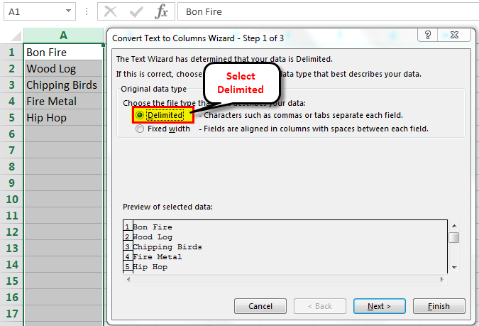
Step 3: Select “space” as the delimiter and click “finish.”

Step 4: The text strings of column A are split into two columns. The second half of the strings is placed in column B. The spaces between the strings have also been removed.

#3 – “Fixed Width” Option of Text to Columns Wizard
The “fixed width” option of the text to columns wizard helps remove extra spaces from numerical and textual data in Excel. For this, all the strings before the space should contain the same number of characters.
The following data contains random text and numbers with spaces in column A. We want to remove the spaces and split the strings into two separate columns.
Use the “fixed width” option of the text to columns wizard.

Step 1: Select column A. In the Data tab, click “text to columns” from the “data tools” group. The same is shown in the following image.
Step 2: The “convert text to columns wizard” appears, as shown in the following image. Select the option “fixed width” in “choose the file type that best describes your data.” Click “next.”

Step 3: Place the cursor at the position of the space. Click “finish.”

Step 4: The strings of column A are split into two columns. The second half of the strings is placed in column B. The spaces between the strings have also been removed.

Note: The text to columns wizard (methods #2 and #3) splits the data into different columns.
#4 – Find and Replace Option
The find and replaceFind and Replace is an Excel feature that allows you to search for any text, numerical symbol, or special character not just in the current sheet but in the entire workbook. Ctrl+F is the shortcut for find, and Ctrl+H is the shortcut for find and replace.read more option helps remove spaces from numerical and textual data in Excel.
Working on the excel data under the heading “TRIM function” (method #1), we want to remove spaces with the find and replace option.

Step 1: Press “Ctrl+H” and the “find and replace” dialog box is displayed, as shown in the following image.

Step 2: Enter a space in the “find what” box. Leave the “replace with” box blank. Click “replace all.”

Step 3: Excel displays a message stating the number of replacements. Click “Ok.”

Step 4: All the spaces in column A have been removed, as shown in the following image.

#5 – SUBSTITUTE Function
The SUBSTITUTE functionSubstitute function in excel is a very useful function which is used to replace or substitute a given text with another text in a given cell, this function is widely used when we send massive emails or messages in a bulk, instead of creating separate text for every user we use substitute function to replace the information.read more helps remove the spaces by replacing them with the existing data string.
Working on the data under the heading “TRIM function” (method #1), we want to remove spaces in excel with the SUBSTITUTE function.

Step 1: In cell B1, enter the SUBSTITUTE function. Click “insert function” in the Formulas tab. The “function arguments” dialog box appears, as shown in the following image.
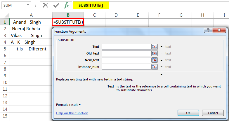
Step 2: Since the text in which characters are to be substituted is present in cell A1, enter the same in the “text” box.

Step 3: Since extra spaces are to be removed, enter “ ” in the “old_text” box. The blank between a pair of double quotation marks refers to a space.

Step 4: Since the space character is to be replaced with the existing text, enter “” in the “new_text” box. The pair of double quotation marks with no character in-between implies no spaces. Click “Ok.”

Step 5: The extra spaces from the name are removed in cell B1, as shown in the following image.

Step 6: Copy or drag the formula to the remaining cells, as shown in the following image.

Note: The find and replace option and the SUBSTITUTE function (methods #4 and #5) display the entire text string together without spaces.
Frequently Asked Questions
What does it mean to remove spaces in excel and why is it important?
While working with Excel, there might be extra spaces that are not easily visible to the user. It is important to eliminate them for the following reasons:
• The spaces at inappropriate places can make the data look untidy and disordered.
• The extra spaces have a negative impact on the quality of data presentation.
• The unwanted spaces can mess up with the formulas of Excel.
• Two cells with and without spaces are considered different entries even though the data in both may be identical.
Since it is difficult to remove the extra spaces manually, there are various techniques available in Excel for such deletions.
How to remove the leading and trailing spaces in Excel with the TRIM function?
Leading spaces are the extra space characters entered at the beginning of a data string. In contrast, the trailing spaces are found at the end of a string without any character following them.
The TRIM function helps remove all the unwanted spaces of the database. The exception to this rule is the single space character inserted between the words.
The syntax of the TRIM function is stated as follows:
“TRIM(text)”
The “text” represents the cell from which excess spaces are to be removed.
For example, the text string “ Chicago, United States ” in cell C2 is changed to “Chicago, United States” by the formula “=TRIM(C2).”
How to remove all the spaces in Excel?
To remove all the spaces in Excel, use the following formula:
“=SUBSTITUTE(C2,“ ”,“”)”
The space (“ ”) is replaced by the existing data (“”) in the cell C2.
For example, the text string “Chicago, United States” in cell C2 is changed to “Chicago,United States” by the given formula.
Note: Alternatively, the find and replace option can be used to remove all the spaces of a data string.
Recommended Articles
This has been a guide to removing spaces in excel cells. We discuss how to remove Leading, Trailing, Blank, Extra Spaces along with step by step examples. You may download an Excel template from the website. For more on Excel, take a look at the following articles –
- Randomize List ExcelRandomizing a list in excel means selecting a random value from the data, to randomize a whole list in excel. There are two excel formulae for this: the =RAND() function, which returns any random value to the cell and then allows us to sort the list, and the =RANDBETWEEN() function, which returns random values to the cell from a number range specified by the user.read more
- Hiding an Excel ColumnThe methods to hide columns in excel are — hide columns using right-click option, hide columns using shortcut cut key, hide columns using column width, hide columns using VBA code.read more
- Hide Formula in ExcelHiding formula in excel is used when we do not want the formula to be displayed in the formula bar when we click on a cell with formulas. We can format the cells, check the hidden checkbox, and protect the worksheet.read more
- Copy Sheet in ExcelThere are various ways to Copy or Move Sheets in Excel 1- By using the dragging method. 2 — By using the right-click method. 3 — Copy a sheet by using Excel Ribbon. 4- Copy Sheet from Another Workbook. and 5- Copy Multiple Sheets in Excel.read more