
This article will walk you through setting up and using the Excel Functions Translator add-in. The Functions Translator is geared towards people who use versions of Excel in different languages, and need help finding the right function in the right language, or even translating entire formulas from one language to another.
The Functions Translator:
-
Enables users who know Excel’s English functions to become productive in localized Excel versions.
-
Enables users to easily translate full formulas to their native language.
-
Supports all of Excel’s localized languages and functions, with 80 languages, and 800 functions.
-
Provides an efficient way to search for any part of a function’s name in both languages selected.
-
Displays a scrollable, and categorized list of English functions, and their corresponding localized functions.
-
Enables you to give feedback to Microsoft on the function translation quality. You can give feedback on a specific function in a specific language.
-
Has been localized for English, Danish, German, Spanish, French, Italian, Japanese, Korean, Dutch, Portuguese Brazilian, Russian, Swedish, Turkish, Chinese Traditional and Chinese Complex Script.
Installing the Functions Translator add-in
The Functions Translator is available for free from the Microsoft Store, and can be installed by following these steps:
-
Start Microsoft Excel.
-
Go to the Insert tab.
-
Click on the Store button in the Ribbon.
-
This will launch the Office Add-ins dialog. Make sure that Store is selected at the top, and then click Productivity on the left-hand side.
-
Search for «Functions Translator» in the upper-left search box.
-
When you find it, click the green Add button on the right, and the translator will be installed
Configuring the Functions Translator
When the Functions Translator has been installed, it creates two buttons on the Home tab at the very right.
The buttons will respectively take you to the Reference and Translator panes in the Functions Translator dialog. The exception to that is the first time you run the Functions Translator it will take you to a Welcome pane:
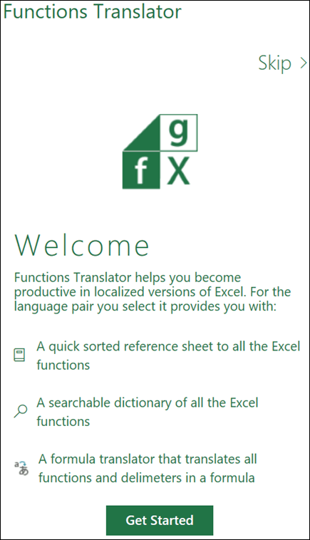
The pane opens at the right-hand side of Excel, which is where it will be anchored for all operations.
You can skip straight to translations by clicking the Skip > link on the right-hand side at the top of the frame, but we recommend selecting Get Started, which will bring you to the Language settings dialog. This allows you to choose your default From and To languages, although you can change them at any time.
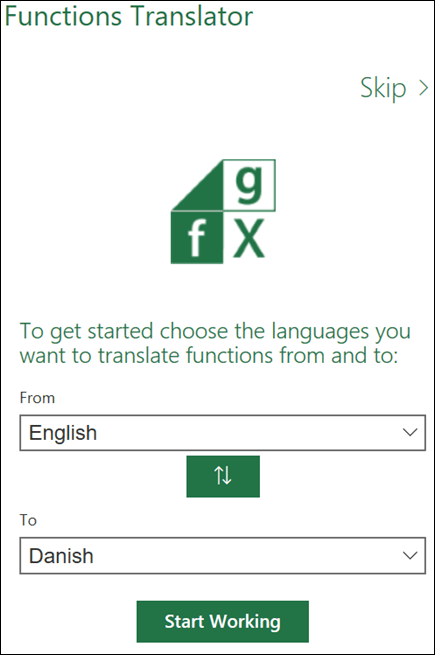
Here you can configure your language set. While the Functions Translator supports all languages that Microsoft has localized Excel functions to, you can only operate with one pair at the time. Any combination of languages is possible, and Excel will remember your choice. The language pair can be changed at any time through the Preferences pane, which is accessible from any of the add-in’s main panes.
By default, the From and To language will be pre-populated with English as the From language and the Excel Install language as the To language. If your install language is one of the languages we have localized for the Functions Translator, the user interface will display in the localized language. Click Start Working when you have selected your language pair.
We are using the concept of To and From in the translator. To is the language that you know, From is the language that you want to find. So if you were researching lookup functions in English, but needed the French function names then you would set the From language to English, and the To language to French.
The green Up arrow/Down arrow button in between To/From has been supplied to let you easily switch the From and To languages around.
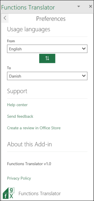
Preferences
You can activate the Preferences pane by clicking the settings wheel at the bottom of any of the three main panes.

Besides providing various links that may be of interest, you can also change your To and From languages from here at any time. Clicking the Left arrow at the top of the pane brings you back to the main pane.
The Reference pane
The Reference Pane has a drop-down list for Function category, which will display all functions in each group selected with the From language on the left, and the To language on the right. If you’re not sure which category a function belongs to, you can choose the All option.
By default, the functions are sorted alphabetically by the From column, in this case English, and shown here with a small down arrow next to the word English. You can sort alphabetically, reverse alphabetically, and you can chose to sort on either the From or To language. Just click on the language you want to sort by, and click on the name again to reverse sort. The arrow indicates the sort direction.
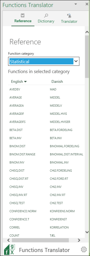
Clicking on a function name in either column will bring you to the Dictionary pane, which will show the function with a short description.
The Dictionary Pane
The Dictionary pane enables you to search for any part of a function name by displaying all functions that contain the letters you entered. For performance reasons, search won’t populate any results until you have entered at least two letters. Search will be in the language pair you have selected, and returns results for both languages.

Once search has returned the function name you want, you can click on it, and the language pair and function definition will be displayed. If you click on a function name in the Reference pane, you will likewise be brought to the Dictionary, and shown the language pair and function description.
Notes:
-
Not all functions will have descriptions, but very few will be missing.
-
Function descriptions are in English only.
-
If you need to see a localized description, you can go to the Formulas tab, click on the relevant Function Category, and hover over the function in question. Excel will display a description of the function in your install language.
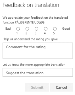
Clicking the lightbulb icon in the Dictionary pane will bring you to the Feedback on translation pane, where you can give us feedback about a particular translation.
The Translator Pane
The Translator pane can translate a full formula from one language to another. Here is an example of the Translator pane where a formula has been translated from English to French:
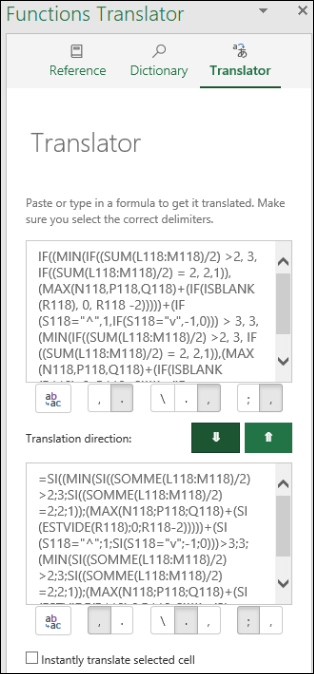
The top box is for the From language, and the bottom for the To language. The two green arrow buttons in the middle will translate in the direction indicated. In this case, we pasted a formula into the From box, and clicked the down arrow to translate to French.
Manually setting delimiters
Excel functions rely on delimiters to separate ranges and arguments from each other. Different languages use different separators, so while the Functions Translator will try to make the right choices, it may sometimes be necessary to set some of these manually.
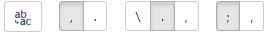
Below each From/To box there are a group of buttons, shown above. The first button will take whatever is in the text box above, and paste it to the currently active cell in Excel. You can use that to paste a localized formula into the cell of your choice.
The other buttons are grouped by their respective functions: the decimal separator, the array separator and the list separator.
-
Decimal separator
-
The decimal separator can either be a period or a comma.
-
-
Array separator
-
This separator is specific to Array formulas.
-
-
List separator
-
For English, the decimal separator is normally a period, and the list delimiter is a comma. For some European languages, the decimal separator is a comma, and the list delimiter therefore has to be something else, namely a semi-colon.
-
Instantly translate selected cell
The Instantly translate selected cell option on the Translator tab will attempt to translate the formula in any cell that you select. It will input the formula from the selected cell into the bottom To language box, and instantly paste a translation in the From language box.
Notes:
-
The Instantly translate selected cell feature is not supported in Microsoft Excel 2013 or earlier.
-
The Instantly translate selected cell feature will not work if you are in Edit mode in a cell. As soon as you exit Edit mode, instant translation will work again.
Feedback
We hope that the Functions Translator helps you to become more productive using localized versions of Excel, and we very much welcome feedback. Please feel free to give feedback on both on functions where the translation may not be the best, but also with the add-in itself.
If you have an opinion on how we localize functions in general, and how you would like to see this add-in work, we would very much like to hear that opinion as well!
The Functions Translator team, Martin and Vadym
fxlator@microsoft.com
Note: We will review each piece of feedback personally, however, we cannot guarantee a response. Please do not include any files containing personal information.
Need more help?
You can always ask an expert in the Excel Tech Community or get support in the Answers community.
If you ever wondered how to translate excel spreadsheets into another language.
This blog will give you a clear guidance on how to do exactly that.
Translation is more than just changing words from one language to another. Translation builds bridges between cultures.
English is a language that is pretty much everywhere. However, solely operating in English can hold back companies and businesses.
There is no question that English is a widely spoken language. A lot of those numbers, though, are made up of people who speak English as a second language. This would mean that most people would actually respond better if they were spoken to in their native language.
These people do understand and comprehend English. They have no problems piecing together words to form a sentence in response to whatever you are asking them. But until you speak the language that their heart speaks (their native language), you won’t really be communicating with them in the most optimal way
Most people simply prefer their native language. It is what they are most comfortable with and it shows in their confidence when they’re speaking. This is why we need translation; it will allow people to communicate more effectively.
With all that being said, it can clearly be seen that translation is more important than the attention and credit it is given. So many people around the world have already benefited from the effects of good and clear translation with its importance is becoming increasingly more well-known today.
In this article I will explain how to translate in Excel with 3 different options:
Table of Contents
Translation through the Review Tab
In this example, I have in column A some words in English that I want to translate into 5 different languages.

You can download the exercise file and follow along by clicking Here. I start at the Review worksheet, where I have in column A some words in English. Select the range A2:A12 and copy it (CTRL + C). Click on the “Review” Tab of the ribbon then click on “Translate”. Alternatively, you can use the shortcut ALT + SHIFT +F7

The Translator pane opens on the right side and shows the selected text in the upper box. English language is automatically detected.
From the lower drop list select the target language, I selected French. Text is instantly translated

Put the mouse cursor in the lower box and hit CTRL + A to select all the translated text, then copy it CTRL + C
Pasting the translated text in cell B2, will result in pasting all the words in one single cell.
To solve the problem, Double click in Cell B2 (the Enter mode of Excel) ► Paste CTRL +V ► Then select all CTRL+A ► Cut the selected translated text CTRL + X ► deselect cell B2 by clicking on a different cell ► Re-select cell B2 ►and Paste CTRL + V … voila. Each word appears in a different cell.
Now, repeat the process for each one of the other languages.

Translating Functions
Translating functions follows a totally different process.
We start by adding a Microsoft Add-in called Functions Translator.
On the Insert Tab click on Get Add-ins.

Click on “Store” ► Select “Productivity” ► then scroll down to “Functions Translator” ► Click Add.
![]()
A window opens ►Click continue to accept the License terms

The tool is added to the right side of the Home Tab, showing 2 options Reference & Translator (both will open the same pane). Click on Reference.

The first time you use the functionality, a Welcome screen allows you to select the languages. You can change the language later one by clicking on the gear icon in the lower right corner of the reference tab.
I have English selected as a source language and German as a target language.

The Reference tab also allows you to select a Function category ► Financial Functions are shown along with the corresponding name in German.
When I clicked on the PMT function ► it switched to the “Dictionary” Tab where it shows a description of the selected function.

To translate any function (including nested functions) go to the “Translator” tab.
In the upper box, type your function (You cannot click on cells in the worksheet to use them as references). Alternatively, if you already have the function in the worksheet, copy it from the formula bar and paste it in the same box.
You can download the exercise file and follow along by clicking Here.
In the “Functions” Worksheet, I copied the PMT function in B5 from the formula bar and I pasted it in the box ► Click on the down pointing arrow for the Translation direction ► you get the translation in German in the lower box

Since delimiters vary from one language to another, you have a set of controls for changing the delimiters.
Test with a different function (the LEFT function) in cell B9.
Test with a Dynamic Array function (TEXTAFTER) in cell C9.

Note if you click on the Replace button to replace the original function with the translated one, this action cannot be undone. But you can always click again on the upper replace button to bring the function in the original language.
But what about nested functions? They work perfectly fine.
I have in cell F19 a VLOOKUP function with a nested CHOOSE function. I copied it from the formula bar and pasted it in the upper box ► I clicked on the down arrow for the Translation direction and the result is amazing.

If at anytime you don’t want the Functions Translator in Excel, you can remove it by going to the Insert Tab ► Click on My Add-ins ► The Office Add-ins dialog box opens ► Select Functions Translator ► Click on the ellipsis ► Click on Remove ► Confirm by hitting Remove ► Then close.

Dynamic Translation using Power Query

I also created a second table in column C (C1:C2) named “Language” for the destination language, or the Target language (tr). C2 is a drop list, that allows me to select any target language.
In cells C4:C5 I created a third table that returns the abbreviated code of the selected language in C2. I named the table “Code” and I used a VLOOKUP function to return that code from a table array named “AllLanguages”.
=VLOOKUP(C2,AllLanguages,2,0)
Here is the “AllLanguages” named range in a hidden sheet named “Data”
You can get the full list of ISO-639.2 codes from the url:
ISO 639-2 Language Code List Codes for the representation of names of languages (Library of Congress) (loc.gov)

The Concept
Load the “Language” table to power Query. Data Tab ► From Table Range ► Right click the single value and select ► Drill Down ► you get a single text value.


On the Home Tab of the query editor : Close & Load To ► Only Create a connection

Repeat the previous steps for the “Code” table. Drill Down ► Load as a connection only.
Solution
On the Data Tab ►Get Data ► From Other Sources ► Blank Query.

Name the Query ”Translate”.
On the Home Tab of the Query Editor ► Click on Advanced Editor ► Delete everything ► Then copy and Paste this code.
					let
    fnTranslate =
        (Shorts as text) as text =>
 let
    Source = Json.Document(
Web.Contents("https://translate.googleapis.com/translate_a/single?client=g
tx&sl=en&tl=" & Code & "&dt=t&q=" & Shorts)
    ),
    Translation = Source{0}{0}{0}
    in
    Translation,
Source = Excel.CurrentWorkbook(){[Name="Shorts"]}[Content],
 ChangeDataType = Table.TransformColumnTypes(Source,{{"English",
type text}}),
 Result = Table.AddColumn(
    ChangeDataType,language,
    each fnTranslate([English]),
    type text
)
in
 Result

Let’s break down this code:
A table is sent from Excel to Power Query.
Power Query connects to Google Translate through an API (Application Programming Interface), a software that allows 2 applications to interact with each other.
The same API reads data from the webservice which returns translated data in JSON format (JavaScript Object Notation).
Since it’s a free API, limit the number of requests by not refreshing the query often and keeping the translation table short.
To access the Free Google Translation API use the URL:
https://translate.googleapis.com/translate_a/single?client=gtx&sl=en&tl=fr&dt=t&q=%22Text
In this URL there are 3 parameters:
Sl ► stands for Source language ISO code.
Tl ► stands for Target Language ISO Code.
Q ► is the text to be translated
The API endpoint returns a JSON file (in array format) that contains French translation(fr) for text given in English
We rename this array Source
					let
 Source =
Web.Contents("https://translate.googleapis.com/translate_a/single?client=g
tx&sl=en&tl=" & Code & "&dt=t&q=" & Shorts)
in
 Source

We need to parse this JSON file to access the translated text.
Json.Document is the function which is responsible of parsing the JSON content. The result is stored in a variable “Translation”
					let
 Source = Json.Document(
 Web.Contents("https://translate.googleapis.com/translate_a/single?client=g
tx&sl=en&tl=" & Code & "&dt=t&q=" & Shorts) ),
 Translation = Source{0}{0}{0}
 in
 Translation,
Note, Source{0}{0}{0} is the first item in the translated text we want to get.
As soon as we run the query, we will be notified to specify how we would like to connect to the web service unless you already defined permission for the Google Translation API endpoint. Click on the Edit Credentials button ► I selected Anonymous
To make this code reusable, I encapsulated it in a Custom function fnTranslate(). We can create the custom function in a separate code and call it in other queries.
Here is my code where I replaced: the target Language by the query named Code, the name of the source table by Shorts, and the column header of the translated text by the query Language.
					let
 fnTranslate =
 (Shorts as text) as text =>
 let
 Source = Json.Document(
Web.Contents("https://translate.googleapis.com/translate_a/single?client=g
tx&sl=en&tl=" & Code & "&dt=t&q=" & Shorts) ),
 Translation = Source{0}{0}{0}
 in
 Translation,
 Source = Excel.CurrentWorkbook(){[Name="Shorts"]}[Content],
 ChangeDataType = Table.TransformColumnTypes(Source,{{"English",
type text}}),
 Result = Table.AddColumn(
 ChangeDataType,Language,
 each fnTranslate([English]),
 type text
 )
 in
 Result

Close and Load To the same Excel worksheet in cell E1
Test by changing the destination language from the drop list in Excel. Every time we select a different target language we need to refresh the query either by:
- Clicking on Refresh All on the Data Tab
- Using the shortcut: CTRL + ALT + F5
- Right-click the sheet tab ► View Code. Copy and paste the following Change Event Code.
					Private Sub Worksheet_Change(ByVal Target As Range)
If Not Intersect(Target, Range("C2:C5")) Is Nothing Then
 ThisWorkbook.RefreshAll
 End If
End Sub
Watch the Full Tutorial on my YouTube channel by clicking here below.
As I am not familiar with all these languages, I wish to hear back from you in a comment; how accurate the translation is.
If you enjoyed the article and the accompanying Video tutorial share it on your social platforms for the benefit to spread.
Переводит содержимое указанной ячейки с одного языка на другой, используя онлайн-переводчик Google

Синтаксис
=Translate(Text; FromLang; ToLang)
где:
- Text – исходная ячейка с текстом для перевода
- FromLang – текстовый двухбуквенный код языка, с которого производится перевод (т.е. язык исходного текста), например «ru», «en», «es», «fr» и т.д.
- ToLang – текстовый двухбуквенный код языка, на который нужно перевести.
Подсмотреть необходимые коды языков можно на странице Google Переводчика в адресной строке после выбора нужных языков в форме:

Примечания
Естественно, данная функция требует подключения к интернету и при его отсутствии выдает ошибку.
При использовании в большом количестве ячеек одновременно, может вызывать замедление работы, т.к. будет выполнять много одновременных запросов. В этом случае рекомендуется заменять формулы на значения при помощи специальной вставки или инструмента В значения.
Полный список всех инструментов надстройки PLEX
Переводчик функций в Excel
В этой статье вы настроили и использовали надстройки Excel Переводчик функций. Функция Переводчик ориентирована на людей, которые используют версии Excel на разных языках, и требуют помощи в поиске нужной функции на нужном языке или даже переводе целых формул с одного языка на другой.
Помогает пользователям, знакомым с английскими функциями Excel, продуктивно работать с локализованными версиями Excel.
Позволяет пользователям полностью переводить формулы на родной язык.
Поддерживает все локализованные языки и функции Excel (80 языков и 800 функций).
Обеспечивает эффективный поиск любой части имени функции на обоих выбранных языках.
Отображает прокручиваемый список по категориям для английских функций и соответствующие локализованные функции.
Позволяет отправить корпорации Майкрософт отзыв о качестве перевода функций. Вы можете оставить отзыв о той или иной функции на любом из доступных языков.
Локализован на английский, датский, немецкий, испанский, французский, итальянский, японский, корейский, нидерландский, португальский (Бразилия), русский, шведский, турецкий и китайский (традиционное письмо и набор сложных знаков) языки.
Установка надстройки «Переводчик функций»
Надстройка Переводчик функций доступна бесплатно в Microsoft Store. Чтобы установить ее, выполните указанные ниже действия.
Запустите приложение Microsoft Excel.
Перейдите на вкладку Вставка.
Нажмите кнопку Магазин на ленте.
Откроется диалоговое окно «Надстройки Office». В верхней части окна выберите пункт Магазин, а слева — Производительность.
Введите в поле поиска запрос Functions Translator.
Нажмите зеленую кнопку Добавить справа от найденной надстройки «Переводчик функций». Она будет установлена.
Настройка Переводчика функций
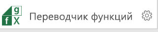
После установки надстройки Переводчик функций на вкладке Главная справа появятся две новых кнопки.

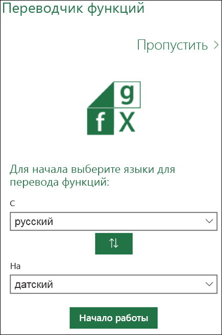
Они открывают в диалоговом окне Переводчик функций области Справочник и Переводчик соответственно. Исключением является первый запуск надстройки Переводчик функций — в этом случае открывается область Добро пожаловать:

Рабочая область Переводчика функций всегда открывается в правой части Excel.
Вы можете перейти непосредственно к переводу, щелкнув ссылку Пропустить > в правом верхнем углу, но мы рекомендуем нажать кнопку Приступим, чтобы перейти в диалоговое окно языковых параметров. Здесь вы можете выбрать языки С и На по умолчанию (их можно изменить в любое время).
Здесь вы можете указать языковые параметры. Хотя Переводчик функций поддерживает все языки, на которые локализованы функции Excel, в каждом случае вы можете использовать только пару из них. Доступно любое сочетание языков, и приложение Excel запомнит ваш выбор. Вы в любое время можете изменить языковую пару в области Настройки, которую можно открыть во всех основных областях Переводчика функций.
По умолчанию в качестве языка «С» и «На» будут заранее заполнены английский язык с языком «От», а языком установки Excel языком «На». Если язык установки является одним из языков, локализованных для Переводчик,пользовательский интерфейс будет отображаться на локализованных языках. Выберите языковую пару, нажав кнопку Начать работу.
В переводчике используются параметры С и На. С — это язык, который вы знаете, На — это язык, перевод на который вам нужен. Так, если вы используете для поиска функций английский язык, но хотите найти их имена на французском языке, то для параметра С нужно выбрать английский язык, а для параметра На — французский.
С помощью зеленой кнопки Стрелка вверх/стрелка вниз между параметрами «С» и «На» можно менять языки С и На местами.
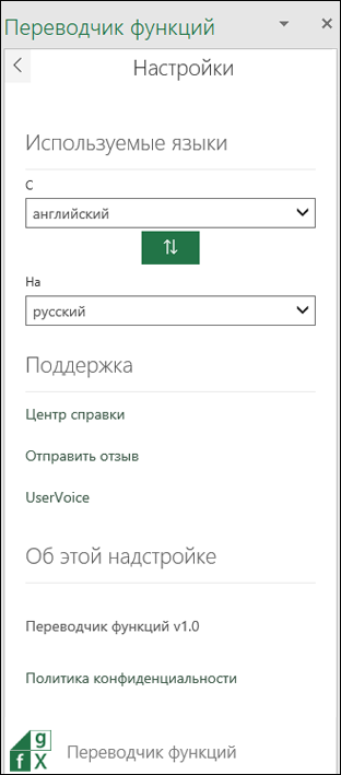
Вы можете открыть область Настройки, щелкнув значок настроек в правом нижнем углу любой из трех основных областей.
Кроме того, вы можете в любое время изменить языки На и От, которые могут быть вам интересны. Если щелкнуть стрелку влево в верхней части области, вы вернетсяе в главную.
Область «Справочник»
В области Справочник есть раскрывающийся список Категория функций, с помощью которого можно отобразить все функции в указанной категории для языков С (слева) и На (справа). Если вы не знаете, к какой категории относится функция, можно использовать параметр Все.
По умолчанию функции сортируются в алфавитном порядке языка С (в данном случае английского), рядом с которым отображается маленькая стрелка вниз. Вы можете сортировать функции в обычном или обратном алфавитном порядке, а также выбирать язык сортировки ( С или На). Просто щелкните название языка, по которому нужно отсортировать функции, а для сортировки в обратном порядке щелкните его еще раз. Стрелка указывает направление сортировки.
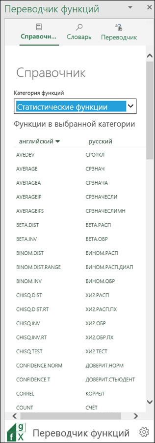
Щелкните имя функции в одном из столбцов, чтобы открыть область Словарь с кратким описанием функции.
Область «Словарь»
В области Словарь можно искать любые части имени функции, отображая все функции, содержащие введенные буквы. По соображениям производительности поиск не будет заполнять результаты, пока вы не ввели хотя бы две буквы. Поиск будет искаться в выбранной языковой паре и возвращать результаты для обоих языков.
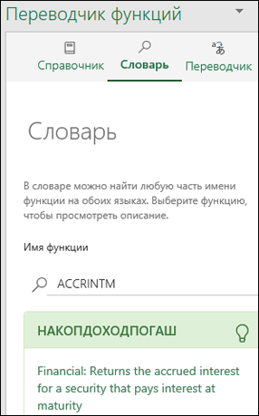
Обнаружив нужное имя функции, вы можете щелкнуть его, чтобы отобразить языковую пару и определение функции. Если щелкнуть имя функции в области Справочник, также откроется область Словарь с указанием языковой пары и описания функции.
У некоторых функций нет описаний.
Описания функций предоставляются только на английском языке.
Чтобы посмотреть локализованное описание, перейдите на вкладку «Формулы», щелкните нужную категорию функций и наведите указатель мыши на требуемую функцию. В Excel отобразится описание функции на языке установки.
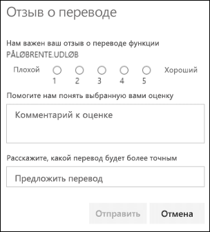
Щелкните значок лампочки в области Словарь, чтобы открыть область Отзыв о переводе, где вы можете оставить отзыв об определенном переводе.
Область «Переводчик»
В области Переводчик можно полностью перевести формулу с одного языка на другой. Ниже приведен пример области Переводчик, где формула переведена с английского языка на французский:
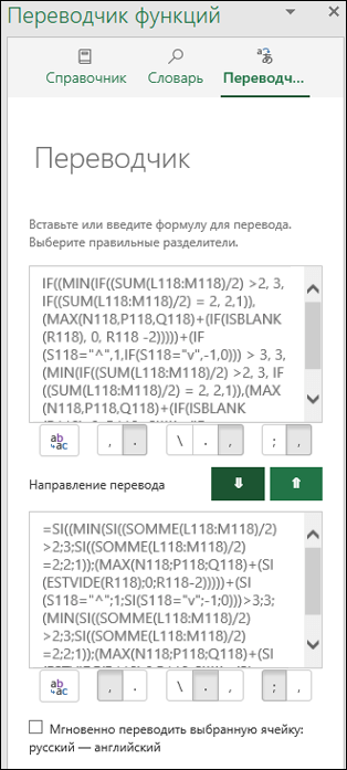
Верхнее поле предназначено для языка С, нижнее — для языка На. Две зеленые кнопки со стрелками между этими полями выполняют перевод в указанном направлении. В примере мы вставили формулу в поле для языка С и нажали кнопку со стрелкой вниз, чтобы перевести формулу на французский язык.
Ручная настройка разделителей
В функциях Excel для разделения диапазонов и аргументов используются разделители. В каждом языке используются свои разделители, и Переводчик функций пытается подобрать нужный вариант, но иногда разделители следует выбирать вручную.

Под полями для языков «С» и «На» отображаются показанные выше кнопки. Первая кнопка вставляет текст из поля выше в активную ячейку. Эту кнопку можно использовать для вставки локализованной формулы в нужную ячейку.
Остальные кнопки распределены по соответствующим функциям: десятичный разделитель, разделитель столбцов для формул массива и разделитель элементов списка.
Десятичным разделителем может быть точка или запятая.
Разделитель столбцов для формул массива
Этот разделитель используется в формулах массива.
Разделитель элементов списка
С английским языком в качестве десятичного разделителя обычно используется точка, а в качестве разделителя элементов списка — запятая. В некоторых европейских языках десятичным разделителем является запятая, а разделителем элементов списка другой символ, а именно точка с запятой.
Мгновенно переводить выбранную ячейку
Если установлен флажок Мгновенно переводить выбранную ячейку в области Переводчик, надстройка будет пытаться перевести формулу в любой выбираемой ячейке. Она будет копировать формулу из выбранной ячейки в поле языка На и мгновенно переводить ее в поле языка С.
Функция Мгновенно переводить выбранную ячейку не поддерживается в Microsoft Excel 2013 и более ранних версий.
В режиме правки функция Мгновенно переводить выбранную ячейку не активна. При выходе из режима правки функция мгновенного перевода активируется снова.
Отзывы и предложения
Мы надеемся, что надстройка Переводчик функций поможет вам эффективнее работать с локализованными версиями Excel, и будем рады вашим отзывам. Сообщите нам о функциях, перевод которых можно улучшить, и поделитесь мнением о работе самой надстройки.
Если у вас есть предложения по поводу улучшения работы надстройки и локализации функций в общем, обязательно отправьте их нам!
Команда Переводчика функций, Мартин и Вадим
Примечание: Мы рассмотрим каждый отзыв индивидуально, но не можем гарантировать ответ на каждый отзыв. Не включайте в отзыв файлы, содержащие личные сведения.
Дополнительные сведения
Вы всегда можете задать вопрос специалисту Excel Tech Community или попросить помощи в сообществе Answers community.
Translator
The Microsoft Excel functions have been localized into many languages. If you send your Excel file to someone using a different language for Excel than you, the functions and formulas used in the workbook are automatically translated by Excel when opening the file. However, the automatic translation usually does not work, if you directly insert foreign language formulas into your worksheet. Such a situation may for example occur, if you are using Excel in German and want to use an English formula provided by a forum. The following online tool allows you to translate an Excel formula from one language into another language and therefore use the localized formula.
Использование редакторов формул в режиме онлайн

Способ 1: Wiris
Wiris — самый продвинутый из всех онлайн-сервисов, о которых пойдет речь в данной статье. Его особенность заключается в том, что он состоит сразу из нескольких модулей, предназначенных для редактирования формул разных форматов. Это позволит абсолютно каждому пользователю отыскать подходящий для себя инструмент и вписать необходимые значения. Предлагаем разобраться с общим принципом взаимодействия с данным сайтом.
-
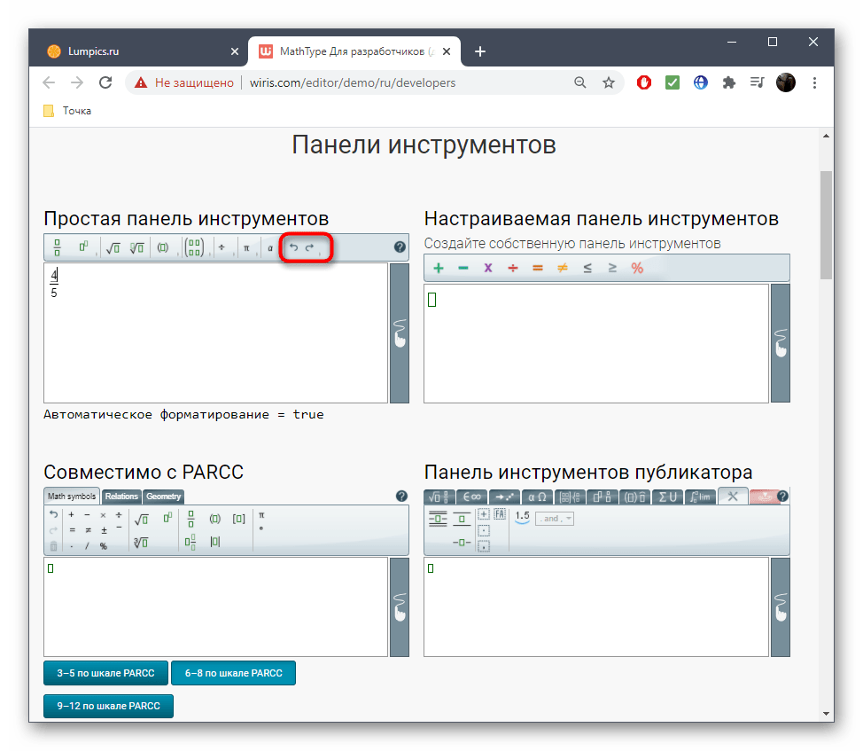
Воспользуйтесь ссылкой выше, чтобы перейти на главную страницу сайта. Здесь вы увидите первый блок редактора, который называется «Простая панель инструментов».

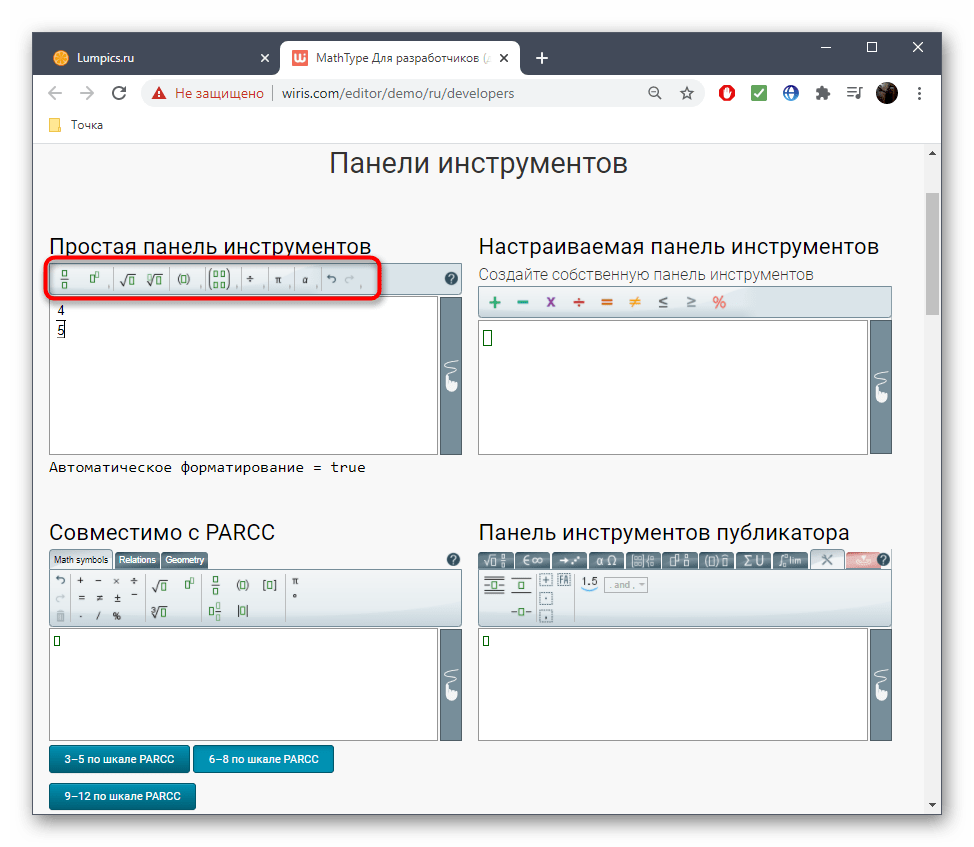
Щелкните левой кнопкой мыши по одному из инструментов, чтобы добавить его в редактор, а затем активируйте курсор на том самом квадрате и впишите туда требуемое число.

Если какое-то действие нужно отменить, примените для этого специальную виртуальную кнопку с изображением стрелочки.

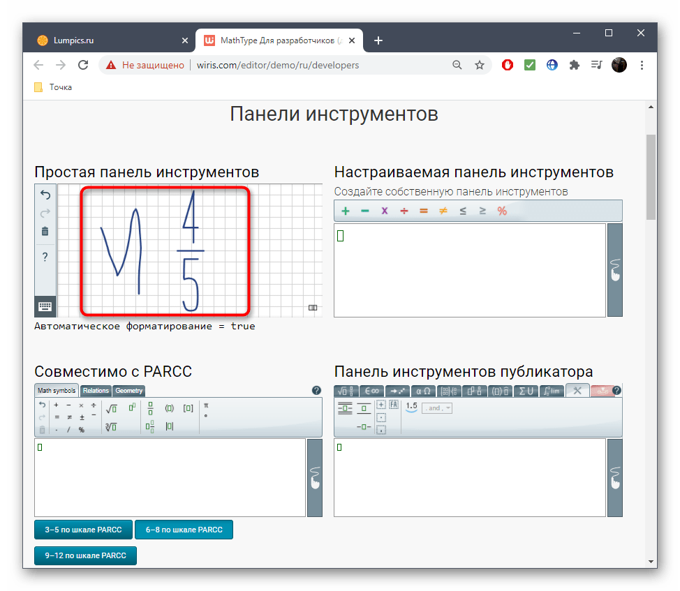
При переходе в этот режим откроется небольшой лист в клеточку, где и осуществляется написание всех чисел, аргументов и прочего содержимого формул. При необходимости вернитесь назад в классическое представление.
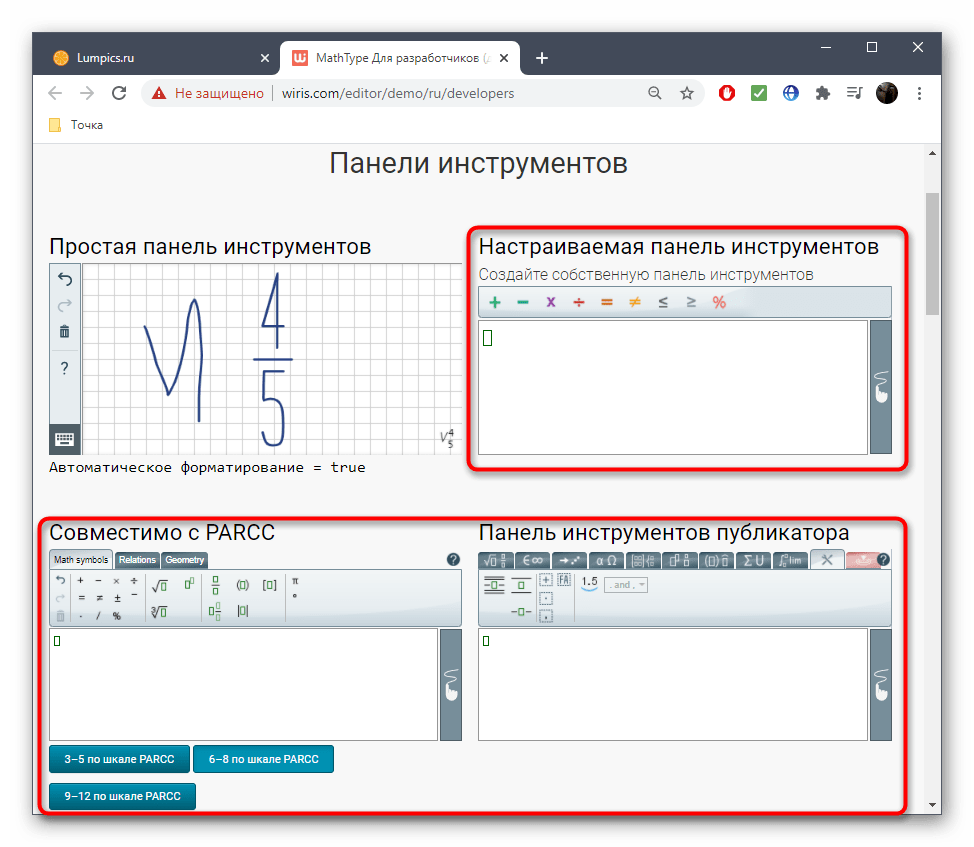
Посмотрите на названия следующих трех блоков. Два из них индивидуальные и подходят для PARCC и публикаторов, а третья панель является настраиваемой, где разработчики позволяют добавить только те инструменты, которые нужны для редактирования именно сейчас.
Опустившись ниже, вы найдете блок «Экспортируйте математические уравнения в разные форматы». Если хотите сохранить формулу в виде отдельного файла, обязательно составляйте ее через данную панель.


Еще ниже есть блок, позволяющий форматировать стандартное представление в LaTeX, однако о таком типа подачи формул мы еще поговорим ниже.

Wiris — идеальное средство для редактирования формул в режиме онлайн. Однако некоторым пользователям такая расширенная функциональность не нужна или присутствующие инструменты попросту не подходят. Тогда мы советуем воспользоваться одним из двух следующих методов.
Способ 2: Semestr
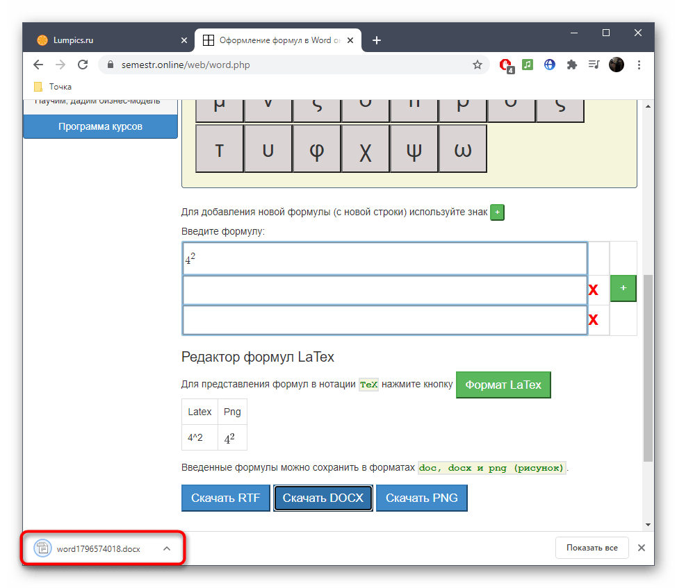
Сайт Semestr предназначен для оформления формул в Word, однако подойдет и для других целей, поскольку разработчики не ставят ограничений на загрузку файла на компьютер, предлагая дополнительно и поддержку перевода в LaTeX.
-
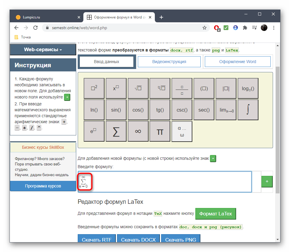
Все доступные составляющие формул располагаются на панели, разделенной на блоки. Соответственно, там, где вы видите пустые квадраты, должны присутствовать числа, вписываемые вручную.
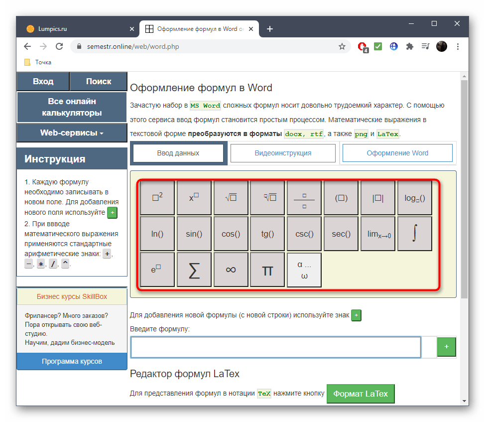
При нажатии по конкретной кнопке ее содержимое сразу же добавляется в блок формулы. Добавляйте другие числа и редактируйте присутствующие по необходимости.

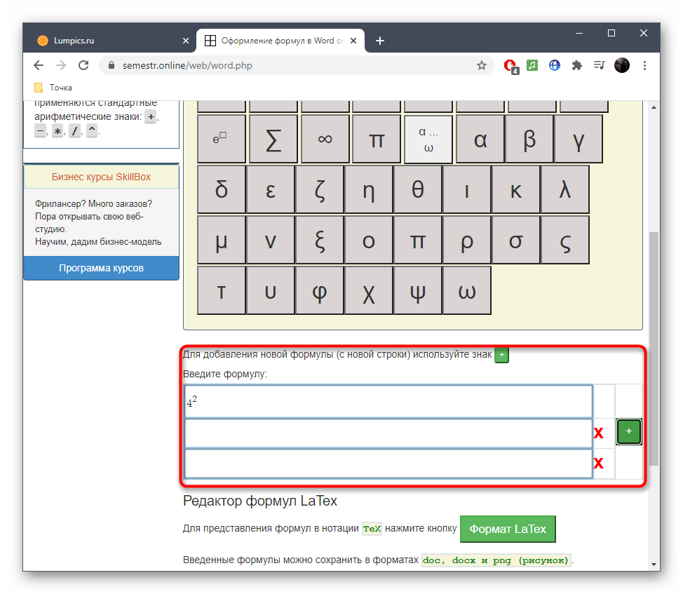
Есть в Semestr и весь греческий алфавит, буквы которого тоже могут понадобиться при составлении формул. Разверните блок с ним, чтобы использовать конкретный символ.

Нажимайте по кнопке с плюсом для добавления новых формул в список. Они будут независимы друг от друга, однако сохранятся как один файл, который в будущем можно вставить в любую программу или использовать для других целей.
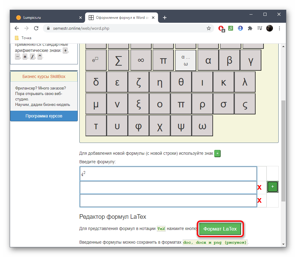
При надобности перевести содержимое в LaTeX кликните по соответствующей зеленой кнопке, а встроенный в Semestr алгоритм выполнит весь процесс автоматически.
После перевода скопируйте полученную формулу или скачайте ее.
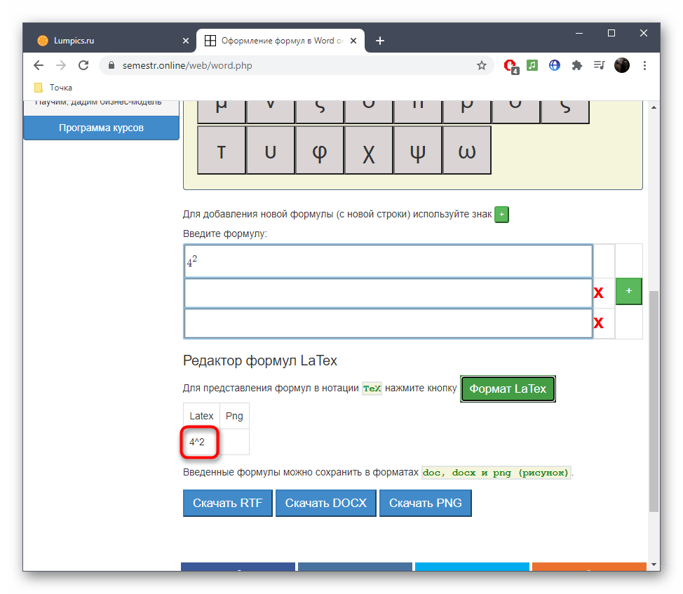
Перед загрузкой выбирайте формат, в котором хотите получить файл, нажав по подходящей кнопке.

Ожидайте завершения загрузки, а затем переходите к дальнейшему взаимодействию с формулами.
Способ 3: Codecogs
Сайт под названием Codecogs оптимален для тех пользователей, кто создает формулы с необходимостью дальнейшего перевода их в формат LaTeX или в тех ситуациях, когда редактирование уже осуществляется в таком форматировании. Codecogs позволяет добавлять различные составляющие формул с одновременным отображением их в классическом варианте и упомянутом выше.
-
Оказавшись на главной странице сайта Codecogs, ознакомьтесь с верхней панелью, откуда и осуществляется добавление всех элементов. Нажмите по одному из блоков, чтобы развернуть доступные варианты или сразу же поместить его в поле.

В редакторе вы увидите представление в LaTeX и сможете вписывать необходимые числа.

Ниже отображается классическое представление, которое в будущем и можно будет сохранить отдельным файлом на компьютере.

Используйте дополнительные функции настройки внешнего вида, чтобы поменять шрифт, фон или размер текста.

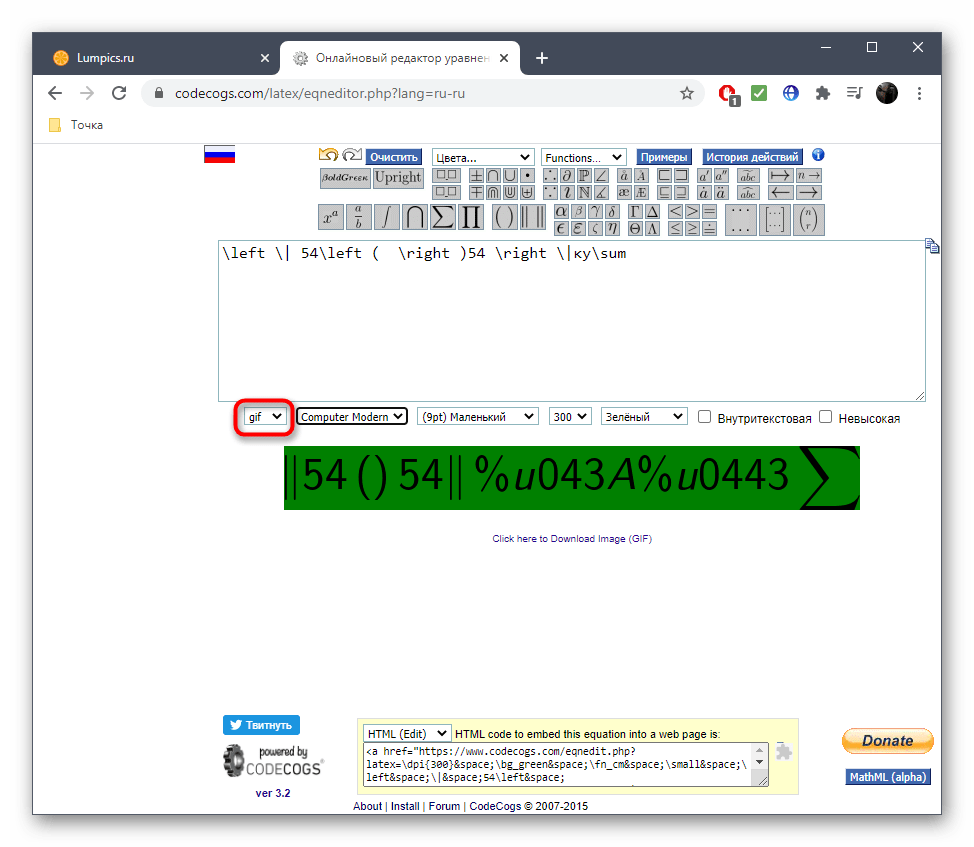
Дополнительно в выпадающем меню выберите формат, в котором файл будет сохранен на жестком диске.
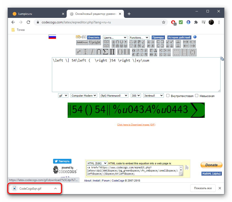
Нажмите по специально отведенной кликабельной надписи для начала загрузки файла с готовой формулой в выбранном формате.
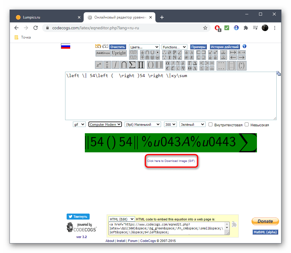
Дождитесь конца скачивания и пользуйтесь готовым уравнением.
Отметим, что для редактирования LaTeX лучше всего использовать отдельные редакторы, которые специально предназначены для этого. Более детальную информацию по этому поводу вы найдете в другой статье на нашем сайте, кликнув по ссылке ниже.
Помимо этой статьи, на сайте еще 12701 инструкций.
Добавьте сайт Lumpics.ru в закладки (CTRL+D) и мы точно еще пригодимся вам.
Отблагодарите автора, поделитесь статьей в социальных сетях.
источники:
http://ru.excel-translator.de/translator/
http://lumpics.ru/formula-editor-online/

If you and your team use versions of Excel in different languages, check out the Functions Translator. This Microsoft add-in can translate entire formulas or help you find the function you want in the language you need.
Install the Functions Translator Add-In
The Functions Translator is a Microsoft add-in available for free. You can install it by heading to the Insert tab and choosing “Get Add-ins” in the Add-ins section of the ribbon.

Enter “Functions Translator” in the Search field and the top. Then select “Add” when you see the add-in in the search results and “Continue” to install it.
Once the add-in installs, you’ll get a new section of the ribbon on the Home tab. On the right, look for Functions Translator and you’ll see the two tools you’ll use, Reference and Translator.
Set Up the Functions Translator
When you install and open the Functions Translator for the first time using either ribbon button, you’ll see a Welcome screen in the side panel on the right. This allows you set up default To and From languages, but you can change these translation languages anytime as needed.
Select Get Started to head to the language settings. If you prefer to get right to work, you can choose “Skip” on the top right.
To set your default languages, simply select them in the drop-down boxes and click “Start Working.”
To change the languages later, select an option in the ribbon and click the gear icon in the sidebar to open the Preferences.
Find a Function
If you want to find a function in another language, click “Reference” in the Functions Translator section of the ribbon on the Home tab.
RELATED: How to Alphabetize Data in Microsoft Excel
This sends you directly to the Reference tab in the tool’s sidebar. Use the drop-down box at the top to pick a category for the function or use “All” to see them all.
The functions appear in alphabetical order so you can find the one you need easily. You’ll see the languages at the top of the list with From on the left and To on the right.
For additional information about a function, select it. You’ll then see a description of the function on the Dictionary tab.
You can also use the Dictionary tab on its own to search for any function you like and see the description and corresponding function in another language.
Translate a Formula
Maybe you’d like to translate a formula, the handiest feature of the tool. Plus, you can use a few convenient options in the Translator area. Click “Translator” in the Functions Translator section of the ribbon on the Home tab.
RELATED: How to Paste Text Without Formatting Almost Anywhere
In the sidebar, either type or paste your formula in the box at the top. Optionally, select the delimiters you want to use.
Then, click the translate button which is the one with the arrow pointing down. You’ll then see your formula translated to the other language in the box at the bottom. You can also do the reverse if necessary and translate the opposite direction using the arrow pointing up button.
To use the translated formula in your sheet, select a cell and then click the icon on the left of the translation. This appears as letters.
To automatically translate a formula in a cell, check the box at the bottom of the sidebar for Instantly Translate Selected Cell. Note the direction of the translation with the To and From languages before doing so.
Whether you need a formula in your own language from a sheet in a different dialect or want to help your team create formulas in their language, the Functions Translator in Excel is a great helper.
READ NEXT
- › How to Translate Languages in Google Sheets
- › How to Install Unsupported Versions of macOS on Your Mac
- › Microsoft Outlook Is Adding a Splash of Personalization
- › This 64 GB Flash Drive From Samsung Is Just $8 Right Now
- › Why Your Phone Charging Cable Needs a USB Condom
- › Liquid Metal vs. Thermal Paste: Is Liquid Metal Better?
- › The Best Steam Deck Docks of 2023
How-To Geek is where you turn when you want experts to explain technology. Since we launched in 2006, our articles have been read billions of times. Want to know more?