
If you have a worksheet with data in columns that you need to rotate to rearrange it in rows, use the Transpose feature. With it, you can quickly switch data from columns to rows, or vice versa.
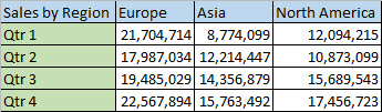
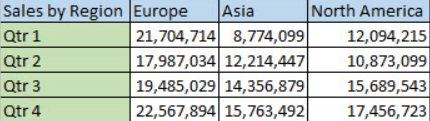
For example, if your data looks like this, with Sales Regions in the column headings and and Quarters along the left side:
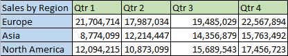
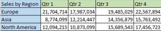
The Transpose feature will rearrange the table such that the Quarters are showing in the column headings and the Sales Regions can be seen on the left, like this:
Note: If your data is in an Excel table, the Transpose feature won’t be available. You can convert the table to a range first, or you can use the TRANSPOSE function to rotate the rows and columns.
Here’s how to do it:
-
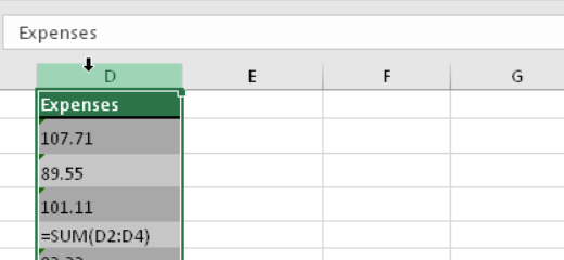
Select the range of data you want to rearrange, including any row or column labels, and press Ctrl+C.
Note: Ensure that you copy the data to do this, since using the Cut command or Ctrl+X won’t work.
-
Choose a new location in the worksheet where you want to paste the transposed table, ensuring that there is plenty of room to paste your data. The new table that you paste there will entirely overwrite any data / formatting that’s already there.
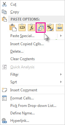
Right-click over the top-left cell of where you want to paste the transposed table, then choose Transpose
 .
.
-
After rotating the data successfully, you can delete the original table and the data in the new table will remain intact.
Tips for transposing your data
-
If your data includes formulas, Excel automatically updates them to match the new placement. Verify these formulas use absolute references—if they don’t, you can switch between relative, absolute, and mixed references before you rotate the data.
-
If you want to rotate your data frequently to view it from different angles, consider creating a PivotTable so that you can quickly pivot your data by dragging fields from the Rows area to the Columns area (or vice versa) in the PivotTable Field List.
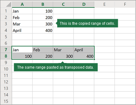
You can paste data as transposed data within your workbook. Transpose reorients the content of copied cells when pasting. Data in rows is pasted into columns and vice versa.
Here’s how you can transpose cell content:
-
Copy the cell range.
-
Select the empty cells where you want to paste the transposed data.
-
On the Home tab, click the Paste icon, and select Paste Transpose.
Excel is a popular and handy tool for storing mathematical, statistical, and other information. Does Excel provide any functionalities for data transformation? Of course, it does! To transform data in Excel, you can use multiple functions, as well as native and third-party tools to automate processes. Read on to learn about all the available options.
What is data transformation in Excel?
According to Wikipedia:
Data transformation is the process of converting data from one format or structure into another format or structure.
So, you basically change the format without changing the information content of the data. The goal of data transformation is to present the data so that it can be used most effectively.
Data transformation in Excel means the same process but implemented in Excel and with the help of Excel functions and tools. For example, you can remove a column, change the data type, or filter rows. Each of these operations means data transformation.
In what cases may data transformation in Excel be needed?
Often, simply arranging data alphabetically, in ascending order, or transforming non-normal data in Excel is not enough. To understand the information, sometimes more complex transformations are required.
After conducting any sociological research, the collected data needs to be grouped in one place, and a detailed analysis should be carried out. Entrepreneurs use Excel data transformation to create reports or optimize their work. These can be companies that are engaged in sales or even tour operators.
If we talk about mathematics or physics, the systematization of data allows them to simplify the work as much as possible. And if, when working with data, you can immediately calculate the square root or raise a number to a power, it makes the work faster. It is almost impossible to list all areas where data transformation in Excel can be used, but to name a few:
- Reporting
- Analysis of statistical data
- Performing mathematical operations with a large amount of data
- Compiling financial data
- Business analytics, and many others
Each specialty can use data transformation in different ways, depending on their goals and needs.
What can you use to transform data in Excel?
Suppose you are planning to transform data values in Excel. In that case, you can take advantage of the numerous Excel functions, as well as built-in and third-party tools.
Excel functions
As for data transformation, Excel itself has a vast number of functions that allow you to transform data, change the spreadsheet’s appearance, perform various mathematical operations, and many others. These functions are more than enough to help you structure and organize your data in most simple cases.
Power Query
Power Query is a popular Excel tool used to extract, transform, and load data. It can be used as part of a self-service ETL solution to perform the following tasks:
- Extract data from the source.
- Transform your data to prepare it for analysis.
- Load the transformed data into a worksheet or data model.
Its massive popularity is in part due to its easy use. All steps are performed automatically, and the final results are recorded in a spreadsheet already familiar to you.
Power Pivot
This is an Excel-like user interface to a full-fledged SQL database installed on your computer and is a powerful tool for processing vast amounts of data. Power Pivot allows you to:
- Link imported spreadsheets by key columns.
- Filter and sort them.
- Perform mathematical and logical operations using more than 150 functions of the built-in DAX language.
Power View
Power View made its way into Excel 2013 from SharePoint. It primarily provides the user with tools for quickly creating live visual reports using pivot spreadsheets and database-based charts.
You can add totals to the report in a simple spreadsheet, a pivot spreadsheet, and various types of charts. Power View allows you to link data from spreadsheets even to Bing maps.
Coupler.io
Coupler.io is not a data transformation tool but a solution for importing data from different apps and sources to Excel. However, you can use it for data transformation purposes in many ways since it allows you to:
- Merge data from different spreadsheets.
- Select columns or a data range for import.
- Import queries (for specific data sources), and many more.
Check out the list of available Excel integrations and find the one you need.
Note: if you did not find the desired source, please fill out this form to let us know which application you would like to import data from.
What are the data transformation functions in Excel?
There are a considerable number of Excel data transformation functions. Here are 10 of the most popular ones:
| Function | Description |
|---|---|
| LOG10 | Allows you to calculate the logarithm to base 10. |
| ASIN | Allows you to calculate the arcsine. |
| SQRT | Allows you to calculate the square root. |
| ABS | Returns the absolute value of a number |
| LET | Assigns names to the results of calculations to allow storage of intermediate calculations, values, or name definitions in a formula. |
| ARABIC | Converts Roman numerals to Arabic numerals as a number. |
| DATE | Returns the sequential serial number that represents a particular date. |
| DAYS | Returns the number of days between two dates. |
| DEGREES | Converts radians to degrees. |
| ISO.CEILING | Rounds a number up to the nearest integer or multiple. |
Each function can perform one or more actions. You are unlikely to have to use all the existing functions. On average, one person uses 3 to 10 different functions, depending on what field of activity they work in.
Example of transforming data in Excel
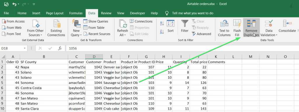
One of the simplest examples of data transformation in Excel is removing duplicates. In Excel, you can do this either with Power Query if you’re getting data from an external source or with a button if your data set is already in Excel. Here is an example of a data set with duplicate records.

To remove these duplicates, click the Remove Duplicates button on the Data tab, then select the columns that contain duplicates.
There you go!

Examples of transforming data using Excel functions and tools
How to transform data into log in Excel?
Users working with stats or scientists or other researchers need to calculate the logarithm of a certain number. It can be quickly done if you use a calculator, but what if there is a large amount of data, and you need to do everything as soon as possible? Then, use log transform data in Excel. To convert the required data to a logarithm, you can use two functions: LOG and LOG 10.
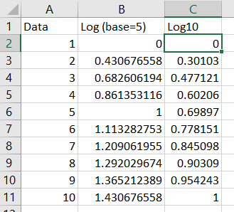
- LOG10 is the function to return the base-10 logarithm of a number.
=log10(number)
- LOG is the function to return the logarithm of a number to the base you specify. The default base value is 10.
=log(number,base)
For example, here are two log transform formulas:
How to square root transform data in Excel?
To apply the square root transformation to a data set in Excel, you can use the SQRT function.
=SQRT(number)
For example:

How to make cube root Excel data transformation?
There is no dedicated function in Excel for cube root transformation. However, you can apply the following formula:
=[value]^(1/3)
For example:
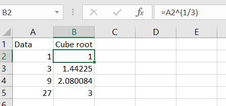
According to this principle, you can perform root transformations of any degree, replacing 3 with the degree you need.
How to arcsine transform data in Excel?
The arcsine is the angle whose sine is the number. The arcsine transform can be used to stretch points between 0 and 1, for example, when working with proportions or fractions.
The arcsine transformation or the angular transformation is calculated as two times the arcsine of the square root of the proportion. To transform such data, use a combination of two functions: ASIN, which returns the inverse sine of a number, and SQRT.
=ASIN(SQRT())
For example, it looks like this:
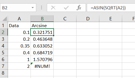
The formula only works for the values in the range from 0 to 1. For example, it returned a #NUM! error for value 2. To avoid this, you will need to convert values to fit the 0 to 1 range. For this, divide each value by the max value into the data set using the following formula:
=[value]/MAX([data-set])
For example:

Nest this formula with the arcise one and you’ll get the proper result, for example:
=ASIN(SQRT(A2/MAX(A2:A6)))

How to transform data in Excel from columns to rows?
Use the transpose function if you have a worksheet with data in columns that need to be rotated to change its row order. With it, you can quickly switch data from columns to rows or vice versa.
Suppose you had a data set like this:
The transpose function rearranges the data set so that it looks like this:
To perform this transformation, you should select the range of data you want to reorder, including any row or column labels, and press Ctrl+C.
Next, you need to select a new location on the worksheet to insert the transposed data set (make sure you have enough space). The new data set that you insert here will completely overwrite any data/formatting already there.
Right-click the top-left cell to paste the transposed data set, then select Transpose.

Once you’ve transformed data in Excel, you can delete the original data set, and the data in the new one will remain intact.
How to transform into numeric data in Excel?
Sometimes, data in Excel is textual, which can lead to some problems. Fixing this is easy enough. You should select the cells and click on the diamond icon with an exclamation mark to select the conversion option to get started. You can perform such actions if this button is not available.

You should select the column where this problem occurs (if you don’t want to convert the entire column, you can select multiple cells instead).
On the Data tab, click Text to Columns.
The Text to Columns button is typically used to split a column, but it can also be used to convert a single column of text to numbers.

The remaining steps of the Text to Columns functionality are best for splitting a column. Since you’re just converting text in a column, you can click Apply right away, and Excel will convert the cells.

Press CTRL + 1 (or ⌘ + 1 on Mac). Then choose any format.
How to transform data range in Excel?
At any moment, you can convert the table to a normal range of data on a worksheet.

Right click on the table, select Table => Convert to range.

Main ideas for data transformation in Excel
The value of data transformation in Excel is difficult to overestimate. It can be used in various fields, such as sociology, mathematics, physics, and many other sciences. It solves several problems:
- Transforms data so that it is easier to do calculations
- Allows you to modify tables so that it is more convenient to work with them
- Simplifies data analysis
- Facilitates the creation of various reports and monitoring
Sometimes, it is impossible to perform calculations correctly since the values can be measured in different physical quantities (for example, radians and degrees), or vice versa; we need to perform some rounding. To not do all the conversions manually, you can use the special features of Excel. It allows you to save a lot of time, effort, and energy to deal with more complex and important processes, while computer technology is doing monotonous work.
Basic Excel data transformation rules
When transforming data in Excel, you need to remember the rules for using this spreadsheet:
- Any action can be reversed, so you should never panic.
- Using formulas when working with Excel simplifies working with a spreadsheet, but if you wish, you can do without them in some cases.
- If you work with Google Excel, there is no need to save permanently, but the interface and functions may differ slightly.
- Some add-ons may already be built into your version of the spreadsheet, while others may need to be downloaded. In the second case, use only trusted sites to avoid downloading a computer virus.
The above rules are not complex, and you can easily remember them even before working with a spreadsheet.
What to do if transform data in Excel fails?
In the process of data transformation, you may lose the data partly or entirely, and this may be very problematic. To mitigate losses, it is good to have a backup of the data.
You can store your backup copy in another Excel workbook stored locally or in the cloud. It would also be great to have copies in another spreadsheet app, for example, Google Sheets, or even in a data warehouse, such as Google BigQuery. You can easily automate backups of your data to any of these destinations using Coupler.io. The schedule for data refresh can be customized, which is more than awesome! Try Coupler.io for free and good luck with your data.
-

A content manager at Coupler.io whose key responsibility is to ensure that the readers love our content on the blog. With 5 years of experience as a wordsmith in SaaS, I know how to make texts resonate with readers’ queries✍🏼

Back to Blog
Focus on your business
goals while we take care of your data!
Try Coupler.io
Go to the Data tab in the ribbon. Select Transform Data by Example.
- A list of transformations from the search will be returned.
- Hover your mouse cursor over any of the transformations returned to preview the results.
- You can see a live preview of the transformation results in your data.
Contents
- 1 What does transform data mean in Excel?
- 2 Where is transform in Excel?
- 3 How do you transform data?
- 4 How do you add get & transform data in Excel?
- 5 What is the difference between load and transform data in Excel?
- 6 How do I enable the data option in Excel?
- 7 Why do we transform data?
- 8 What is an Xlookup in Excel?
- 9 Can Excel get data from PDF?
- 10 What are the types of data transformation?
- 11 What is data transformation give example?
- 12 What is transformation with example?
- 13 How can power query transform data?
- 14 How do I load data into a query table in Excel?
- 15 How do I convert data to normal distribution in Excel?
- 16 How do you get data analysis on Excel?
- 17 How do you use data function?
- 18 What are the 4 functions of transforming the data into information?
- 19 How is raw data transformed?
- 20 What are the three most common transformations in ETL processes?
What does transform data mean in Excel?
Transforming data means modifying it in some way to meet your data analysis requirements. For example, you can remove a column, change a data type, or filter rows. Each of these operations is a data transformation.
Where is transform in Excel?
In Excel 2016, they can be accessed through the Data tab, and then the Get & Transform Data section. In Power BI, the functionality exists on the Home tab, in the External Data section.
The Data Transformation Process Explained in Four Steps
- Step 1: Data interpretation.
- Step 2: Pre-translation data quality check.
- Step 3: Data translation.
- Step 4: Post-translation data quality check.
How do you add get & transform data in Excel?
Import data with Power Query (Get & Transform)
- Go to Ribbon > Data > Get Data > From File > From Workbook.
- Power Query displays the Import Data dialog box.
- Identify the source workbook and double-click on it.
- Power Query displays the Navigator dialog box.
- Select the data source you want to work with.
- Click Load.
What is the difference between load and transform data in Excel?
When you load data you can use data directly as you import on power bi desktop. If you use transform you can modify the data you already have or importing data.
How do I enable the data option in Excel?
Show legacy data import wizards
- Select File > Options > Data.
- Select one or more wizards to enable access from the Excel ribbon.
- Close the workbook and then reopen it to see the activate the wizards.
- Select Data > Get Data > Legacy Wizards, and then select the wizard you want.
Why do we transform data?
Data is transformed to make it better-organized. Transformed data may be easier for both humans and computers to use. Properly formatted and validated data improves data quality and protects applications from potential landmines such as null values, unexpected duplicates, incorrect indexing, and incompatible formats.
What is an Xlookup in Excel?
Use the XLOOKUP function to find things in a table or range by row.With XLOOKUP, you can look in one column for a search term, and return a result from the same row in another column, regardless of which side the return column is on.
Can Excel get data from PDF?
Technically, Microsoft built a “PDF data connector” for Excel, which lets end users import PDF table data using the Data tab in Excel. They select “From File” and then “From PDF” to import data.
What are the types of data transformation?
Top 8 Data Transformation Methods
- 1| Aggregation. Data aggregation is the method where raw data is gathered and expressed in a summary form for statistical analysis.
- 2| Attribute Construction.
- 3| Discretisation.
- 4| Generalisation.
- 5| Integration.
- 6| Manipulation.
- 7| Normalisation.
- 8| Smoothing.
What is data transformation give example?
Data transformation is the mapping and conversion of data from one format to another. For example, XML data can be transformed from XML data valid to one XML Schema to another XML document valid to a different XML Schema. Other examples include the data transformation from non-XML data to XML data.
What is transformation with example?
Transformation is the process of changing. An example of a transformation is a caterpillar turning into a butterfly.
How can power query transform data?
These transformations can be as simple as removing a column or filtering rows, or as common as using the first row as a table header. There are also advanced transformation options such as merge, append, group by, pivot, and unpivot.
How do I load data into a query table in Excel?
In Excel, you may want to load a query into another worksheet or Data Model.
- In Excel, select Data > Queries & Connections, and then select the Queries tab.
- In the list of queries, locate the query, right click the query, and then select Load To.
- Decide how you want to import the data, and then select OK.
How do I convert data to normal distribution in Excel?
Creating a Bell Curve in Excel
- In cell A1 enter 35.
- In the cell below it enter 36 and create a series from 35 to 95 (where 95 is Mean + 3* Standard Deviation).
- In the cell adjacent to 35, enter the formula: =NORM.DIST(A1,65,10,FALSE)
- Again use the fill handle to quickly copy and paste the formula for all the cells.
How do you get data analysis on Excel?
Windows
- Click the File tab, click Options, and then click the Add-Ins category.
- In the Manage box, select Excel Add-ins and then click Go.
- In the Add-Ins box, check the Analysis ToolPak check box, and then click OK. If Analysis ToolPak is not listed in the Add-Ins available box, click Browse to locate it.
How do you use data function?
Remarks. You use the SETDATA and GETDATA functions for transferring data in a notification. The functions are typically needed for handling actions on the notification. The SETDATA function is called from the source of the notification, while the GETDATA function is called from the action code.
What are the 4 functions of transforming the data into information?
Take Depressed Data, follow these four easy steps and voila: Inspirational Information!
- Know your business goals. An often neglected first step you have got to be very aware of, and intimate with.
- Choose the right metrics.
- Set targets.
- Reflect and Refine.
How is raw data transformed?
Data transformation is the process of converting data from one format to another. The most common data transformations are converting raw data into a clean and usable form, converting data types, removing duplicate data, and enriching the data to benefit an organization.
What are the three most common transformations in ETL processes?
Let’s dive in and learn how to convert raw data into insights through the three-step ETL process.
- 1st Step – Extraction.
- 2nd Step – Transformation.
- 3rd Step – Loading.
Many statistical tests make the assumption that datasets are normally distributed.
However, this assumption is often violated in practice. One way to address this issue is to transform the values of the dataset using one of the following three transformations:
1. Log Transformation: Transform the values from y to log(y).
2. Square Root Transformation: Transform the values from y to √y.
3. Cube Root Transformation: Transform the values from y to y1/3.
By performing these transformations, the data typically becomes closer to normally distributed. The following examples show how to perform these transformations in Excel.
Log Transformation in Excel
To apply a log transformation to a dataset in Excel, we can use the =LOG10() function.
The following screenshot shows how to apply a log transformation to a dataset in Excel:
![]()
To determine if this transformation made the dataset more normally distributed, we can perform a Jarque-Bera normality test in Excel.
The test statistic for this test is defined as:
JB =(n/6) * (S2 + (C2/4))
where:
- n: the number of observations in the sample
- S: the sample skewness
- C: the sample kurtosis
Under the null hypothesis of normality, JB ~ X2(2).
If the p-value that corresponds to the test statistic is less than some significance level (e.g. α = .05), then we can reject the null hypothesis and conclude that the data is not normally distributed.
The following screenshot shows how to perform a Jarque-Bera test for the raw data and the transformed data:

Notice that the p-value for the raw data is less than .05, which indicates that it is not normally distributed.
However, the p-value for the transformed data is not less than .05, so we can assume that it is normally distributed. This tells us that the log transformation worked.
Square Root Transformation in Excel
To apply a square root transformation to a dataset in Excel, we can use the =SQRT() function.
The following screenshot shows how to apply a square root transformation to a dataset in Excel:

Notice that the p-value of the Jarque-Bera normality test for the transformed data is not less than .05, which indicates that the square root transformation was effective.
Cube Root Transformation in Excel
To apply a cube root transformation to a dataset in Excel, we can use the =DATA^(1/3) function.
The following screenshot shows how to apply a cube root transformation to a dataset in Excel:

The p-value of the Jarque-Bera normality test for the transformed data is not less than .05, which indicates that the cube root transformation was effective.
All three data transformations effectively made the raw data more normally distributed.
Out of the three transformations, the log transformation resulted in the largest p-value in the Jarque-Bera normality test, which tells us that it likely made the data the “most” normally distributed out of the three transformation methods.
Additional Resources
How to Perform a Box-Cox Transformation in Excel
What is the Assumption of Normality in Statistics?
Содержание
- Transpose (rotate) data from rows to columns or vice versa
- Tips for transposing your data
- Need more help?
- Microsoft Excel — The BASICS of Data Transformation
- Key Concepts Essential to Shaping Data For Analysis
- Data Transformation / Shaping Process
- Excel Data Tables
- Step 1-Convert raw data input into an Excel Table
- Step 2 — Create additional fields in the data table
- Step 3 — Populate the Calendar Year field
- Step 4 — Populate the Category Summary field
- Step 5 — Populate the Stratification field
- About Don
- How to Transform Data in Excel (Log, Square Root, Cube Root)
- Log Transformation in Excel
- Square Root Transformation in Excel
- Cube Root Transformation in Excel
- How to Transform Data in Excel? Ultimate Guide
- What is data transformation in Excel?
- In what cases may data transformation in Excel be needed?
- What can you use to transform data in Excel?
- Excel functions
- Power Query
- Power Pivot
- Power View
- Coupler.io
- What are the data transformation functions in Excel?
- Example of transforming data in Excel
- Examples of transforming data using Excel functions and tools
- How to transform data into log in Excel?
- How to square root transform data in Excel?
- How to make cube root Excel data transformation?
- How to arcsine transform data in Excel?
- How to transform data in Excel from columns to rows?
- How to transform into numeric data in Excel?
- How to transform data range in Excel?
- Main ideas for data transformation in Excel
- Basic Excel data transformation rules
- What to do if transform data in Excel fails?
Transpose (rotate) data from rows to columns or vice versa
If you have a worksheet with data in columns that you need to rotate to rearrange it in rows, use the Transpose feature. With it, you can quickly switch data from columns to rows, or vice versa.
For example, if your data looks like this, with Sales Regions in the column headings and and Quarters along the left side:
The Transpose feature will rearrange the table such that the Quarters are showing in the column headings and the Sales Regions can be seen on the left, like this:
Note: If your data is in an Excel table, the Transpose feature won’t be available. You can convert the table to a range first, or you can use the TRANSPOSE function to rotate the rows and columns.
Here’s how to do it:
Select the range of data you want to rearrange, including any row or column labels, and press Ctrl+C.
Note: Ensure that you copy the data to do this, since using the Cut command or Ctrl+X won’t work.
Choose a new location in the worksheet where you want to paste the transposed table, ensuring that there is plenty of room to paste your data. The new table that you paste there will entirely overwrite any data / formatting that’s already there.
Right-click over the top-left cell of where you want to paste the transposed table, then choose Transpose  .
.
After rotating the data successfully, you can delete the original table and the data in the new table will remain intact.
Tips for transposing your data
If your data includes formulas, Excel automatically updates them to match the new placement. Verify these formulas use absolute references—if they don’t, you can switch between relative, absolute, and mixed references before you rotate the data.
If you want to rotate your data frequently to view it from different angles, consider creating a PivotTable so that you can quickly pivot your data by dragging fields from the Rows area to the Columns area (or vice versa) in the PivotTable Field List.
You can paste data as transposed data within your workbook. Transpose reorients the content of copied cells when pasting. Data in rows is pasted into columns and vice versa.
Here’s how you can transpose cell content:
Copy the cell range.
Select the empty cells where you want to paste the transposed data.
On the Home tab, click the Paste icon, and select Paste Transpose.
Need more help?
You can always ask an expert in the Excel Tech Community or get support in the Answers community.
Источник
Microsoft Excel — The BASICS of Data Transformation
Key Concepts Essential to Shaping Data For Analysis
Whenever analysis and reporting is performed in Excel — and practically every company does — it is imperative that data is aggregated correctly and “transformed”.
For analysis to be efficient and effective, proper structure of the data and the development of additional fields (to aid analysis) is very important.
The two charts above were developed for a recent training session I conducted.
A part of the session was to focus on working with a data set I compiled (Apple historical sales) and performing basic data “shaping” to enable flexible analysis and reporting.
Below, I highlight the steps taken to do this and touch on three areas of Excel that are typically used for basic data transformation and analysis:
- Excel Data Tables
- VLOOKUP function
- Pivot Tables (future post…) — Part 2
Data Transformation / Shaping Process
Excel Data Tables
Here is a excellent summary from TechRepublic of key reasons you want to use Excel Tables. Key considerations mentioned include:
- Effortless data entry
- Always visible headers
- Formula autofill (my favorite!)
- Dynamic range
Step 1-Convert raw data input into an Excel Table
Step 2 — Create additional fields in the data table
This will enable the analysis we are potentially interested in getting. In this session, I have anticipated a need for three additional fields.
Step 3 — Populate the Calendar Year field
Step 4 — Populate the Category Summary field
We will use a VLOOKUP with EXACT match to do this. Here is the formula syntax for VLOOKUP.
Step 5 — Populate the Stratification field
Getting this field populated is more complicated. Here’s why:
- It involves 2 lookup tables. Since the Amount field includes $’s AND Units, separate lookup tables are needed for DOLLARS grouping and UNITS grouping.
- Nesting functions is used to resolve this. The formula performs the following:
— Use the IF Function to check whether the TYPE field is “Dollars”.
— If TYPE = “Dollars”, then use the specified lookup table (result if IF statement is TRUE).
— If TYPE is NOT “Dollars”, then use the Units lookup table (result if IF statement is FALSE).
Our data set is complete…for now.
Next step is to start to build analysis and visualizations of the data. This is the fun part — and where pivot tables make it simple!
I will cover the basics tips I provided in the presentation in a future post…stay tuned!
About Don
“On a mission to challenge the status quo to a more productive and effective end…”
Don is passionate about helping professionals and organizations keep up and adapt to the changing business world that we operate in.
Источник
How to Transform Data in Excel (Log, Square Root, Cube Root)
Many statistical tests make the assumption that datasets are normally distributed.
However, this assumption is often violated in practice. One way to address this issue is to transform the values of the dataset using one of the following three transformations:
1. Log Transformation: Transform the values from y to log(y).
2. Square Root Transformation: Transform the values from y to √ y .
3. Cube Root Transformation: Transform the values from y to y 1/3 .
By performing these transformations, the data typically becomes closer to normally distributed. The following examples show how to perform these transformations in Excel.
Log Transformation in Excel
To apply a log transformation to a dataset in Excel, we can use the =LOG10() function.
The following screenshot shows how to apply a log transformation to a dataset in Excel:
![]()
To determine if this transformation made the dataset more normally distributed, we can perform a Jarque-Bera normality test in Excel.
The test statistic for this test is defined as:
JB =(n/6) * (S 2 + (C 2 /4))
- n: the number of observations in the sample
- S: the sample skewness
- C: the sample kurtosis
Under the null hypothesis of normality, JB
If the p-value that corresponds to the test statistic is less than some significance level (e.g. α = .05), then we can reject the null hypothesis and conclude that the data is not normally distributed.
The following screenshot shows how to perform a Jarque-Bera test for the raw data and the transformed data:
![]()
Notice that the p-value for the raw data is less than .05, which indicates that it is not normally distributed.
However, the p-value for the transformed data is not less than .05, so we can assume that it is normally distributed. This tells us that the log transformation worked.
Square Root Transformation in Excel
To apply a square root transformation to a dataset in Excel, we can use the =SQRT() function.
The following screenshot shows how to apply a square root transformation to a dataset in Excel:
![]()
Notice that the p-value of the Jarque-Bera normality test for the transformed data is not less than .05, which indicates that the square root transformation was effective.
Cube Root Transformation in Excel
To apply a cube root transformation to a dataset in Excel, we can use the =DATA^(1/3) function.
The following screenshot shows how to apply a cube root transformation to a dataset in Excel:
![]()
The p-value of the Jarque-Bera normality test for the transformed data is not less than .05, which indicates that the cube root transformation was effective.
All three data transformations effectively made the raw data more normally distributed.
Out of the three transformations, the log transformation resulted in the largest p-value in the Jarque-Bera normality test, which tells us that it likely made the data the “most” normally distributed out of the three transformation methods.
Источник
How to Transform Data in Excel? Ultimate Guide
Excel is a popular and handy tool for storing mathematical, statistical, and other information. Does Excel provide any functionalities for data transformation? Of course, it does! To transform data in Excel, you can use multiple functions, as well as native and third-party tools to automate processes. Read on to learn about all the available options.
What is data transformation in Excel?
According to Wikipedia:
Data transformation is the process of converting data from one format or structure into another format or structure.
So, you basically change the format without changing the information content of the data. The goal of data transformation is to present the data so that it can be used most effectively.
Data transformation in Excel means the same process but implemented in Excel and with the help of Excel functions and tools. For example, you can remove a column, change the data type, or filter rows. Each of these operations means data transformation.
In what cases may data transformation in Excel be needed?
Often, simply arranging data alphabetically, in ascending order, or transforming non-normal data in Excel is not enough. To understand the information, sometimes more complex transformations are required.
After conducting any sociological research, the collected data needs to be grouped in one place, and a detailed analysis should be carried out. Entrepreneurs use Excel data transformation to create reports or optimize their work. These can be companies that are engaged in sales or even tour operators.
If we talk about mathematics or physics, the systematization of data allows them to simplify the work as much as possible. And if, when working with data, you can immediately calculate the square root or raise a number to a power, it makes the work faster. It is almost impossible to list all areas where data transformation in Excel can be used, but to name a few:
- Reporting
- Analysis of statistical data
- Performing mathematical operations with a large amount of data
- Compiling financial data
- Business analytics, and many others
Each specialty can use data transformation in different ways, depending on their goals and needs.
What can you use to transform data in Excel?
Suppose you are planning to transform data values in Excel. In that case, you can take advantage of the numerous Excel functions, as well as built-in and third-party tools.
Excel functions
As for data transformation, Excel itself has a vast number of functions that allow you to transform data, change the spreadsheet’s appearance, perform various mathematical operations, and many others. These functions are more than enough to help you structure and organize your data in most simple cases.
Power Query
Power Query is a popular Excel tool used to extract, transform, and load data. It can be used as part of a self-service ETL solution to perform the following tasks:
- Extract data from the source.
- Transform your data to prepare it for analysis.
- Load the transformed data into a worksheet or data model.
Its massive popularity is in part due to its easy use. All steps are performed automatically, and the final results are recorded in a spreadsheet already familiar to you.
Power Pivot
This is an Excel-like user interface to a full-fledged SQL database installed on your computer and is a powerful tool for processing vast amounts of data. Power Pivot allows you to:
- Link imported spreadsheets by key columns.
- Filter and sort them.
- Perform mathematical and logical operations using more than 150 functions of the built-in DAX language.
Power View
Power View made its way into Excel 2013 from SharePoint. It primarily provides the user with tools for quickly creating live visual reports using pivot spreadsheets and database-based charts.
You can add totals to the report in a simple spreadsheet, a pivot spreadsheet, and various types of charts. Power View allows you to link data from spreadsheets even to Bing maps.
Coupler.io
Coupler.io is not a data transformation tool but a solution for importing data from different apps and sources to Excel. However, you can use it for data transformation purposes in many ways since it allows you to:
- Merge data from different spreadsheets.
- Select columns or a data range for import.
- Import queries (for specific data sources), and many more.
Check out the list of available Excel integrations and find the one you need.
Note: if you did not find the desired source, please fill out this form to let us know which application you would like to import data from.
What are the data transformation functions in Excel?
There are a considerable number of Excel data transformation functions. Here are 10 of the most popular ones:
| Function | Description |
|---|---|
| LOG10 | Allows you to calculate the logarithm to base 10. |
| ASIN | Allows you to calculate the arcsine. |
| SQRT | Allows you to calculate the square root. |
| ABS | Returns the absolute value of a number |
| LET | Assigns names to the results of calculations to allow storage of intermediate calculations, values, or name definitions in a formula. |
| ARABIC | Converts Roman numerals to Arabic numerals as a number. |
| DATE | Returns the sequential serial number that represents a particular date. |
| DAYS | Returns the number of days between two dates. |
| DEGREES | Converts radians to degrees. |
| ISO.CEILING | Rounds a number up to the nearest integer or multiple. |
Each function can perform one or more actions. You are unlikely to have to use all the existing functions. On average, one person uses 3 to 10 different functions, depending on what field of activity they work in.
Example of transforming data in Excel
One of the simplest examples of data transformation in Excel is removing duplicates. In Excel, you can do this either with Power Query if you’re getting data from an external source or with a button if your data set is already in Excel. Here is an example of a data set with duplicate records.
To remove these duplicates, click the Remove Duplicates button on the Data tab, then select the columns that contain duplicates.

Examples of transforming data using Excel functions and tools
How to transform data into log in Excel?
Users working with stats or scientists or other researchers need to calculate the logarithm of a certain number. It can be quickly done if you use a calculator, but what if there is a large amount of data, and you need to do everything as soon as possible? Then, use log transform data in Excel. To convert the required data to a logarithm, you can use two functions: LOG and LOG 10.
- LOG10 is the function to return the base-10 logarithm of a number.
- LOG is the function to return the logarithm of a number to the base you specify. The default base value is 10.
For example, here are two log transform formulas:
![]()
How to square root transform data in Excel?
To apply the square root transformation to a data set in Excel, you can use the SQRT function.
![]()
How to make cube root Excel data transformation?
There is no dedicated function in Excel for cube root transformation. However, you can apply the following formula:
![]()
According to this principle, you can perform root transformations of any degree, replacing 3 with the degree you need.
How to arcsine transform data in Excel?
The arcsine is the angle whose sine is the number. The arcsine transform can be used to stretch points between 0 and 1, for example, when working with proportions or fractions.
The arcsine transformation or the angular transformation is calculated as two times the arcsine of the square root of the proportion. To transform such data, use a combination of two functions: ASIN, which returns the inverse sine of a number, and SQRT.
For example, it looks like this:
![]()
The formula only works for the values in the range from 0 to 1. For example, it returned a #NUM! error for value 2. To avoid this, you will need to convert values to fit the 0 to 1 range. For this, divide each value by the max value into the data set using the following formula:
Nest this formula with the arcise one and you’ll get the proper result, for example:
How to transform data in Excel from columns to rows?
Use the transpose function if you have a worksheet with data in columns that need to be rotated to change its row order. With it, you can quickly switch data from columns to rows or vice versa.
Suppose you had a data set like this:
![]()
The transpose function rearranges the data set so that it looks like this:
![]()
To perform this transformation, you should select the range of data you want to reorder, including any row or column labels, and press Ctrl+C.
Next, you need to select a new location on the worksheet to insert the transposed data set (make sure you have enough space). The new data set that you insert here will completely overwrite any data/formatting already there.
Right-click the top-left cell to paste the transposed data set, then select Transpose.
Once you’ve transformed data in Excel, you can delete the original data set, and the data in the new one will remain intact.
How to transform into numeric data in Excel?
Sometimes, data in Excel is textual, which can lead to some problems. Fixing this is easy enough. You should select the cells and click on the diamond icon with an exclamation mark to select the conversion option to get started. You can perform such actions if this button is not available.
You should select the column where this problem occurs (if you don’t want to convert the entire column, you can select multiple cells instead).
On the Data tab, click Text to Columns.
The Text to Columns button is typically used to split a column, but it can also be used to convert a single column of text to numbers.
The remaining steps of the Text to Columns functionality are best for splitting a column. Since you’re just converting text in a column, you can click Apply right away, and Excel will convert the cells.
Press CTRL + 1 (or ⌘ + 1 on Mac). Then choose any format.
How to transform data range in Excel?
At any moment, you can convert the table to a normal range of data on a worksheet.
Right click on the table, select Table => Convert to range.
Main ideas for data transformation in Excel
The value of data transformation in Excel is difficult to overestimate. It can be used in various fields, such as sociology, mathematics, physics, and many other sciences. It solves several problems:
- Transforms data so that it is easier to do calculations
- Allows you to modify tables so that it is more convenient to work with them
- Simplifies data analysis
- Facilitates the creation of various reports and monitoring
Sometimes, it is impossible to perform calculations correctly since the values can be measured in different physical quantities (for example, radians and degrees), or vice versa; we need to perform some rounding. To not do all the conversions manually, you can use the special features of Excel. It allows you to save a lot of time, effort, and energy to deal with more complex and important processes, while computer technology is doing monotonous work.
Basic Excel data transformation rules
When transforming data in Excel, you need to remember the rules for using this spreadsheet:
- Any action can be reversed, so you should never panic.
- Using formulas when working with Excel simplifies working with a spreadsheet, but if you wish, you can do without them in some cases.
- If you work with Google Excel, there is no need to save permanently, but the interface and functions may differ slightly.
- Some add-ons may already be built into your version of the spreadsheet, while others may need to be downloaded. In the second case, use only trusted sites to avoid downloading a computer virus.
The above rules are not complex, and you can easily remember them even before working with a spreadsheet.
What to do if transform data in Excel fails?
In the process of data transformation, you may lose the data partly or entirely, and this may be very problematic. To mitigate losses, it is good to have a backup of the data.
Источник