
Excel for Microsoft 365 Excel for Microsoft 365 for Mac Excel for the web Excel 2021 Excel 2019 Excel 2016 Excel 2013 Excel 2010 Excel 2007 More…Less
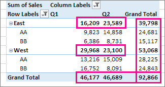
When working with a PivotTable, you can display or hide subtotals for individual column and row fields, display or hide column and row grand totals for the entire report, and calculate the subtotals and grand totals with or without filtered items.

-
In a PivotTable, select an item of a row or column field. Make sure it is a field and not a value.
-
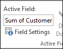
On the PivotTable Analyze tab, in the Active Field group, click Field Settings.

This displays the Field Settings dialog box.
-
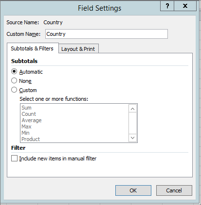
In the Field Settings dialog box, under Subtotals, do one of the following:
-
To subtotal an outer row or column label using the default summary function, click Automatic.
-
To remove subtotals, click None.
Note: If a field contains a calculated item, you can’t change the subtotal summary function.
-
To use a different function, to display more than one type of subtotal, or to subtotal an inner row or column label, click Custom (if this option is available), and then select a function.
Functions that you can use as a subtotal
Function
Description
Sum
The sum of the values. This is the default function for numeric data.
Count
The number of data values. The Count summary function works the same as the COUNTA function. Count is the default function for data other than numbers.
Average
The average of the values.
Max
The largest value.
Min
The smallest value.
Product
The product of the values.
Count Numbers
The number of data values that are numbers. The Count Numbers summary function works the same as the worksheet COUNT function.
StDev
An estimate of the standard deviation of a population, where the sample is a subset of the entire population.
StDevp
The standard deviation of a population, where the population is all of the data to be summarized.
Var
An estimate of the variance of a population, where the sample is a subset of the entire population.
Varp
The variance of a population, where the population is all of the data to be summarized.
Note: You cannot use a custom function that uses an Online Analytical Processing (OLAP) data source.
-
-
To include or exclude new items when applying a filter in which you have selected specific items in the Filter menu, select or clear the Include new items in manual filter check box.
Tips:
-
To quickly display or hide the current subtotal, right-click the item of the field, and then select or clear the check box next to Subtotal «<Label name>».
-
For outer row labels in compact or outline form, you can display subtotals above or below their items, or hide the subtotals, by doing the following:
-
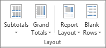
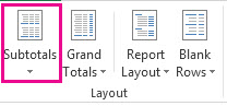
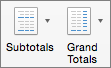
On the Design tab, in the Layout group, click Subtotals.
-
Do one of the following:
-
Select Do Not Show Subtotals.
-
Select Show all Subtotals at Bottom of Group.
-
Select Show all Subtotals at Top of Group.
-
-
You can display or hide the grand totals for the current PivotTable. You can also specify default settings for displaying and hiding grand totals
Display or hide grand totals
-
Click anywhere in the PivotTable.
-
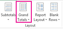
On the Design tab, in the Layout group, click Grand Totals, and then select the grand total display option that you want.
Change the default behavior for displaying or hiding grand totals
-
Click the PivotTable.
-
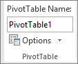
On the PivotTable Analyze tab, in the PivotTable group, click Options.
-
In the PivotTable Options dialog box, on the Totals & Filters tab, do one of the following:
-
To display grand totals, select either Show grand totals for columns or Show grand totals for rows, or both.
-
To hide grand totals, clear either Show grand totals for columns or Show grand totals for rows, or both.
-
-
Click anywhere in the PivotTable.
-
On the PivotTable Analyze tab, in the PivotTable group, click Options.
-
In the PivotTable Options dialog box, on the Total & Filters tab, do one of the following:
-
For Online Analytical Processing (OLAP) source data, do one of the following:
-
Select or clear the Subtotal filtered page items check box to include or exclude report filter items.
Note: The OLAP data source must support the MDX expression subselect syntax.
-
Select or clear the Mark totals with * check box to display or hide an asterisk next to totals. The asterisk indicates that the visible values that are displayed and that are used when Excel calculates the total are not the only values that are used in the calculation.
Note: This option is only available if the OLAP data source does not support the MDX expression subselect syntax.
-
-
For non-OLAP source data, select or clear the Allow multiple filters per field check box to include or exclude filtered items in totals.
-
Need more help?
Want more options?
Explore subscription benefits, browse training courses, learn how to secure your device, and more.
Communities help you ask and answer questions, give feedback, and hear from experts with rich knowledge.
When you create a PivotTable that shows value amounts, subtotals and grand totals appear automatically, but you can also show or hide them.
Show or hide subtotals
-
Click anywhere in the PivotTable to show the PivotTable Tools.
-
Click Design > Subtotals.
-
Pick the option you want:
-
Do Not Show Subtotals
-
Show all Subtotals at Bottom of Group
-
Show all Subtotals at Top of Group
Tip: You can include filtered items in the total amounts by clicking Include Filtered Items in Totals. Click this option again to turn it off. You’ll find additional options for totals and filtered items on the Totals & Filters tab in the PivotTable Options dialog box (Analyze> Options).
-
Show or hide grand totals
-
Click anywhere in the PivotTable to show the PivotTable Tools on the ribbon.
-
Click Design > Grand Totals.
-
Pick the option you want:
-
Off for Rows and Columns
-
On for Rows and Columns
-
On for Rows only
-
On for Columns only
-
Tip: If you don’t want to show grand totals for rows or columns, uncheck the Show grand totals for rows or Show grand totals for columns boxes on the Totals & Filters tab in the PivotTable Options dialog box (Analyze> Options).
When you create a PivotTable that shows value amounts, subtotals and grand totals appear automatically, but you can also show or hide them.
Tip: Row grand totals are only displayed if your data just has one column, because a grand total for a group of columns often doesn’t make sense (for example, if one column contains quantities and one column contains prices). If you want to display a grand total of data from several columns, create a calculated column in your source data, and display that column in your PivotTable.
Show or hide subtotals
To show or hide subtotals:
-
Click anywhere in the PivotTable to show the PivotTable Analyze and Design tabs.
-
Click Design > Subtotals.
-
Pick the option you want:
-
Don’t Show Subtotals
-
Show All Subtotals at Bottom of Group
-
Show All Subtotals at Top of Group
Tip: You can include filtered items in the total amounts by clicking Include Filtered Items in Totals. Click this option again to turn it off.
-

Show or hide grand totals
-
Click anywhere in the PivotTable to show the PivotTable Analyze and Design tabs.
-
Click Design > Grand Totals.
-
Pick the option you want:
-
Off for Rows & Columns
-
On for Rows & Columns
-
On for Rows Only
-
On for Columns Only
-
When a pivot table has grand totals, Excel automatically names those totals. I’ll show you some examples, with details on which grand total headings you can change, and which ones you can’t.
Grand Total Headings Video
This video shows how pivot table Grand Totals are created, and how you can change some of the headings. The detailed instructions are below the video.
Your browser can’t show this frame. Here is a link to the page
The Video Timeline:
0:00 Introduction
0:52 Add a Column Field
1:15 Change the Heading Text
1:55 Add Another Value Field
3:01 Change Total Field Heading
3:51 Get the Excel Workbook
Creating Grand Totals
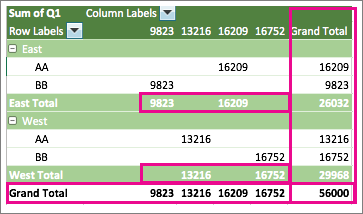
If you create a very simple pivot table, with one Row field and one Value field, Excel will automatically show a Grand Total of the amounts at the bottom.

Then, if you add a field to the Columns area, Excel will show a Grand Total at the right. The headings both have the default text – “Grand Total”.

Change the Grand Total Headings
Sometimes you might want a different Grand Total heading, instead of the default text. For example, if the column contains small numbers, you could put a shorter name at the top. That will let you keep the pivot table as narrow as possible.
In a simple pivot table like this, it’s easy to change the grand total headings – just follow these steps:
- Select either one of the “Grand Total” heading cells
- Then, to change the text:
- Type a new heading, to replace the existing heading
- OR Press F2, then edit in the text in the cell
- OR Click in the Formula bar, and edit the text there
NOTE: You can’t double-click the cell to edit the text.
In the screen shot below, I typed “GT” in cell D4, to create a smaller heading in column D.

As soon you complete the name change, Excel automatically changes the other Grand Total heading, to the same text.

Grand Total Headings – Multiple Values
If there are multiple Value fields in a pivot table, Excel shows a different set of grand total headings.
In the screen shot below, the Order Count field was added to the Values area. Now, instead of a Grand Total column at the right, there are columns with “Total” and the field names – Total Qty and Total Orders
The Row Grand Total, in cell A11, did not change.

Cannot Change Total Field Headings
It was easy to change the original “Grand Total” headings, but Excel won’t let you change these “Total Field” headings
If you try to edit a Total Field heading, an error message will appear: “Cannot edit subtotal, block total, or grand total names.”

Can Still Change Grand Total Headings
However, that error message is a bit misleading. You can’t change the “Total Field” headings, but you CAN still edit the “Grand Total” heading in that pivot table.
In the pivot table shown below, I was able to change the Row “Grand Total” heading, without any problems.

More Pivot Table Grand Total Info
For more information, go to the pivot table Grand Totals page on my Contextures website. See workarounds for showing a grand total at the top or at the left, and other grand total tricks.
_______________
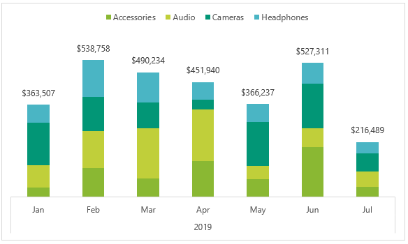
If you work with PivotTables, then you’ve probably found that you can’t include grand totals in Pivot Charts, or subtotals for that matter. And if you’ve ever created a stacked column chart then you’ll have likely wanted to include grand totals as column labels, like this:
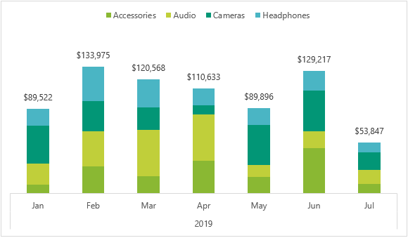
And then remembered you can’t.
One workaround is to create a regular chart from a PivotTable, then you can include the Grand Totals in the source data range.
Another option is to use CUBE functions to connect to the PivotTable source data. The nice thing about CUBE functions is you can get the PivotTable to create them for you and they can retain connectivity to Slicers. That’s right, you don’t even need to learn how to write CUBE formulas!
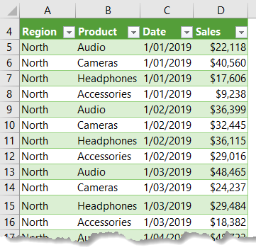
My data, shown below, is formatted in an Excel table called, Table1. It’s product sales by date and region:
Download Workbook
Download the workbook and follow along:
Enter your email address below to download the sample workbook.
By submitting your email address you agree that we can email you our Excel newsletter.
Automatically Create CUBE Formulas
The key to CUBE formulas is that your data needs to be referenced from Power Pivot*, aka the Data Model.
*Power Pivot is available in for Excel 2010, Excel 2013/2016 Office Professional Plus, Office 2016 Professional, any version of Excel 2019 or Office 365, or the standalone edition of Excel 2013/2016. Click here for the full list.
Step 1: Load data to the Data Model
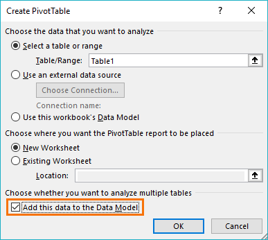
Insert a new PivotTable and at the dialog box check the ‘add this data to the Data Model’ box:
Note: Excel 2010 users will need to load the data to Power Pivot via the Power Pivot tab > Add Linked Table. Then from the Power Pivot window Home tab > Insert PivotTable.
Step 2: Build the PivotTable
Create the PivotTable that will support your Pivot Chart. I like to insert a chart at the same time to make sure the PivotTable layout is going to result in a chart that looks the way I want.
I’m using a stacked column chart, therefore I need the series names in the column labels and the dates in the rows, so they form my horizontal axis labels:
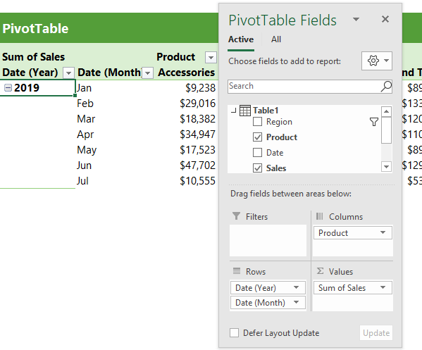
Tip: My dates are grouped into years and months: to do this, right-click the date in the PivotTable > Group.
Optional: If you’d like to filter your chart with a Slicer, insert it now. I’ve inserted a Slicer for the Region field. More on this in step 6.
Step 3: Convert the PivotTable to CUBE Formulas
Select any cell in the PivotTable > PivotTable Analyze tab > OLAP Tools > Convert to Formulas:
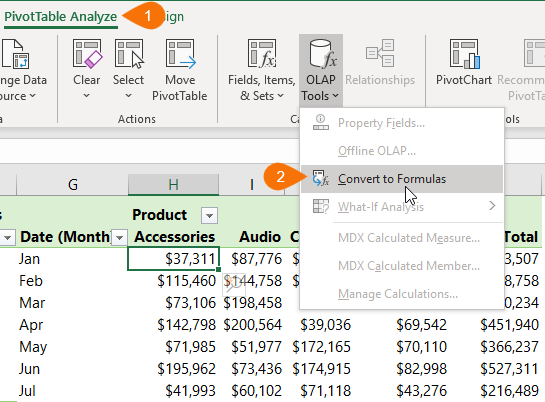
If you inspect the cells in what was your PivotTable, you’ll see they’re now CUBE formulas, as shown below:
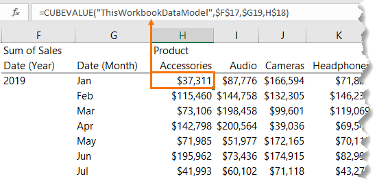
The CUBE formulas are directly referencing the Data Model. Any changes to the Power Pivot Data Model will be reflected in the CUBE formulas.
Step 4: Insert a Regular Chart
Now that you’ve converted the PivotTable to CUBE formulas you can insert a regular chart i.e. not a PivotChart. I’m using a stacked column chart.
Step 5: Format the Chart
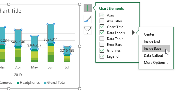
The Grand Total value is the top segment of the stacked column chart. We need to hide this, but first let’s select the grand total series and add Data Labels > Inside Base:
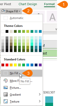
Next, with the grand total series still selected go to the Format tab > Shape Fill > No Fill
Hide the gridlines and vertical axis, and place the legend at the top (be sure to delete the legend entry for ‘Grand Total’; select it in the legend and press the Delete key):
Step 6: Connect CUBE Formulas to Slicers (Optional)
My data set allows me to filter the data by region and I’m going to do this with the Slicer I inserted in step 2.
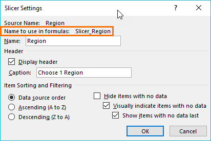
First, right-click the Slicer > Slicer Settings and find its ‘name to use in formulas’:
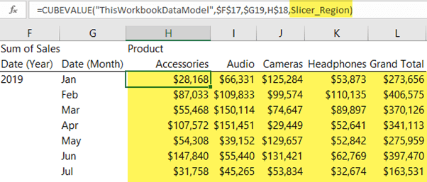
Now, edit the CUBE formulas in the values area to include the Slicer ‘name to use in formulas’ in the next ‘member_expression’ argument, like so:
=CUBEVALUE("ThisWorkbookDataModel",$F$17,$G19,H$18,Slicer_Region)
Be sure to copy the formula to all the values area cells:
Step 7: Format and Arrange Slicer and Chart
Now all that’s left is to align the Slicer to the chart and make it look nice:
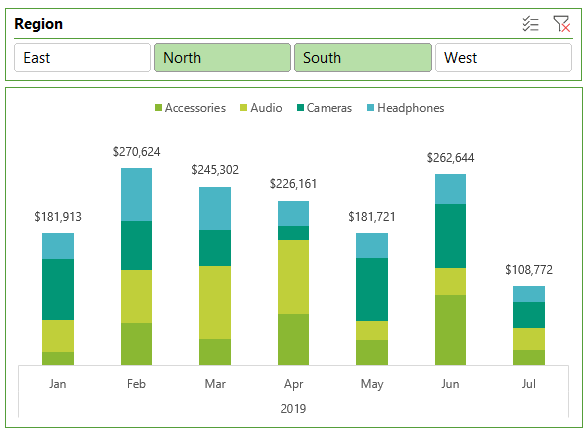
Notice the Slicer acts as a header for the chart and informs the user what regions it relates to without the need for an extra heading.
Tip: This CUBE formula technique also works with PivotTables based on an OLAP data source like SSAS Cubes.
Learn Power Pivot
Power Pivot is hugely versatile and enables you to work with a lot of data and or, data spread across multiple tables. If you’d like to learn Power Pivot please consider my Power Pivot course. There is more information on what Power Pivot can do on the course page linked to above.
You’re likely going to come across the need for running totals if you’re dealing with any sort of daily data.
Imagine you track sales each day. Your data contains a row for each date with a total sales amount, but maybe you want to know the total sales for the month at each day. This is a running total, it’s the sum of all sales up to and including the current days sales.
In this post we’ll cover multiple ways to calculate a running total for your daily data. We’ll explore how to use worksheet formulas, pivot tables, power pivot with DAX and power query.
We’ll also explore what happens to the running total calculation when inserting or deleting rows of data and how to update the results.
Get the file with all the examples.
Running Totals with a Simple Formula
It’s possible to create a basic running total formula using the + operator.
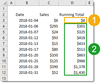
However, we’ll need to use two different formulas to get the job done.
- =C3 will be the first formula and will only be in the first row of the running total.
- =C4+D3 will be in the second row and can be copied down the remaining rows for the running total.
The formula in our first row can’t add the cell above it to the total as it contains a text value for a column heading. This would cause a #VALUE! error to appear in the running total since the + can’t handle text values. We avoid this with a different formula in the first row which doesn’t reference the cell above.
What happens to the running total when we insert or delete rows in our data?
Inserting a new row will result in a gap in the running total. To fix this, we’ll need to copy the formula down from the first cell above the newly inserted rows all the way down to the last row.
Deleting any rows will result in #REF! errors since deleting a row means deleting a cell referenced by the formula below it. To fix this, we’ll need to copy the formula down from the last error-free cell all the way down to the last row.
Running Totals with a SUM Formula
We can avoid the awkwardness of using two different formulas in our running total column by utilizing the SUM function instead of the + operator. When the SUM function encounters a text cell it will treat it the same as a though it contained a 0.
This way we can use the following formula uniformly for every row including the first row.
=SUM(C3,D2)
This formula will reference the column heading containing text for the first row, but this ok as it’s treated like a 0.
When inserting or deleting rows, we will still encounter the same problems with blank cells and errors. We can fix them the same way as with running totals in the simple formula method.
Running Totals with a Partially Fixed Range
Another option with the SUM function is to only reference the Sales column and use a partially fixed range reference.
If we use the following formula =SUM($C$3:C3), we can copy and paste this down the range. It won’t reference any column headings and the range referenced will grow to each row.
Unfortunately, this too will have the same problems (and solutions) with inserting or deleting rows.
Running Totals with a Relative Named Range
We can avoid the problems with inserting and deleting rows from our data if we use a relative named range. This will refer to the cell directly above no matter how many rows we insert or delete.
This is a trick that involves temporarily switching the Excel reference style from A1 to R1C1. Then defining a named range using the R1C1 notation. Then switching the reference style back to A1.
In R1C1 reference style, cells are referred to by how far away they are from the cell using the reference. For example, =R[-2]C[3] refers to the cell 2 up and 3 to the right of the cell using this formula.
We can use this relative referencing to create a named range that’s always one cell above the referring cell with the formula =R[-1]C.
To switch reference style, go to the File tab then choose Options. Go to the Formula section in the Excel Options menu and check the R1C1 reference style box and then press the OK button.
Now we can add our named range. Go to the Formula tab of the Excel ribbon and choose the Define Name command.
Insert a name like “Above” as the name of the range. Add the formula =R[-1]C into the Refers to input and press the OK button.
We can now switch Excel back to the default reference style. Go to the File tab > Options the Formula section > uncheck the R1C1 reference style box > then press the OK button.
Now we can use the formula =SUM([@Sales],Above) in our running total column.
The named range Above will always refer to the cell directly above. When we insert or delete rows, the relative named range will adjust accordingly and no action is needed.
In fact if we place our data in an Excel Table then the formula will automatically fill down for any new rows since the formula is uniform for the entire column. No action is needed to copy down any formulas.
Running Totals with a Pivot Table
Pivot tables are super useful for summarizing any type of data. There’s more to them than just adding, counting and finding averages. There are many other types of calculations built in, and there is actually a running total calculation!
First, we need to insert a pivot table based on the data. Select a cell inside the data and go to the Insert tab and choose the PivotTable command. Then go through the Create PivotTable window to choose where you want the pivot table, either in a new worksheet or somewhere in an existing one.
Add the Date field into the Rows area of the pivot table, then add the Sales field into the Values area of the pivot table. Now add another instance of the Sales field into the Rows area.
We should now have two identical Sales fields with one of them being labelled Sum of Sales2. We can rename this label anytime by simply typing over it with something like Running Total.
Right click on any of the values in the Sum of Sales2 field and select Show Value As then choose Running Total In.
We want to show the running total by date, so in the next window we need to select Date as the Base Field.
That’s it, we now have a new calculation which displays the running total of our sales inside the pivot table.
What happens if we add or delete a row in our source data, how does this affect the running total? The pivot table calculations are dynamic and will take any new data into account in its running total calculation, we will just need to refresh the pivot table.
Right click anywhere inside the pivot table and choose Refresh from the menu.
Running Totals with Power Pivot and DAX Measures
The first couple steps for this are the exact same using a regular pivot table.
Select a cell inside the data and go to the Insert tab and choose the PivotTable command.
When you come to the Create PivotTable menu, check the Add this data to the Data Model box to add the data to the data model and enable it for use with power pivot.
Place the Date field in the Rows area and the Sales field in the Values area of the pivot table.
With power pivot, we will need to create any extra calculations we want using the DAX language. Right click on the table name in the PivotTable Fields window, then select Add Measure to create a new calculation. Note, this is only available with the data model.
=CALCULATE (
    SUM ( Sales[Sales] ),
    FILTER (
        ALL (Sales[Date] ),
        Sales[Date] <= MAX (Sales[Date])
    )
)
Now we can create our new running total measure.
- In the Measure window, we need to add a Measure Name. In this case we can name the new measure as Running Total.
- We also need to add the above formula into the Formula box.
- The cool thing about power pivot is the ability to assign a number format to a measure. We can choose the Currency format for our measure. Whenever we use this measure in a pivot table the format will automatically be applied.
Press the OK button and the new measure will be created.
There will be a new field listed in the PivotTable Fields window. It has a small fx icon on the left to denote that it’s a measure and not a regular field in the data.
We can use this new field just like any other field and drag it into the Values area to add our running total calculation into the pivot table.
What happens to the running total when we add or remove data from the source table? Just like a regular pivot table, we simply need to right click on the pivot table and select Refresh to update the calculation.
Running Totals with a Power Query
We can also add running totals to our data using power query.
First we need to import the table into power query. Select the table of data and go to the Data tab and choose the From Table/Range option. This will open the power query editor.
Next we can sort our data by date. This is an optional step we can add so that if we change the order of our source data, the running total will still appear by date.
Click on the filter toggle in the date column heading and choose Sort Ascending from the options.
We need to add an index column. This will be used in the running total calculation later on. Go to the Add Column tab and click on the small arrow next to the Index Column to insert an index starting at 1 in the first row.
We need to add a new column to our query to calculate the running total. Go to the Add Column tab and choose the Custom Column command.
We can name the column as Running Total and add the following formula.
List.Sum(List.Range(#"Added Index"[Sales],0,[Index]))
The List.Range function creates a list of values from the Sales column starting at the 1st row (0th item) which spans a number of rows based on the value in the index column.
The List.Sum function then adds up this list of values which is our running total.
We no longer need the index column, it has served its purpose and we can remove it. Right click on the column heading and select Remove from the options.
We’ve got our running total and are finished with the query editor. We can close the query and load the results into a new worksheet. Go to the Home tab of the query editor and press the Close & Load button.
What happens with the running total when we add or remove rows from our source data? We will need to refresh the power query output table to update the running total with the changes. Right click anywhere on the table and choose Refresh to update the table.
With the optional sorting step above, if we add dates out of order to the source data, power query will sort by date and return the correct order by date for the running total.
Conclusions
There are many different options for calculating running totals in Excel.
We’ve explored options including formulas in the worksheet, pivot tables, power pivot DAX formulas, and power query. Some offer a more robust solution when adding or removing rows from the data, other methods offer an easier implementation.
Simple formulas in the worksheet are easy to set up but won’t handle inserting or deleting new rows of data easily. Other solutions like pivot tables, DAX and power query are more robust and handle inserting or deleting rows of data easily but are harder to set up.
It’s good to be aware of the pros and cons of each method and choose the one best suited. If you won’t be inserting or deleting new data, then worksheet formulas might be the way to go.
About the Author
John is a Microsoft MVP and qualified actuary with over 15 years of experience. He has worked in a variety of industries, including insurance, ad tech, and most recently Power Platform consulting. He is a keen problem solver and has a passion for using technology to make businesses more efficient.