
If you’ve ever had to sum up items across many different sheets, then you know it can be a real pain when there are a lot of sheets. This trick will make it super easy.
Get the example workbook with the above link to follow along.
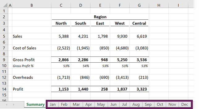
In this example, you have a table of sales figures each in a separate tab named Jan through Dec.
Each sheet is the same format with the table in the same position within each sheet.
=Jan!C3+Feb!C3+Mar!C3+Apr!C3+May!C3+Jun!C3+Jul!C3+Aug!C3+Sep!C3+Oct!C3+Nov!C3+Dec!C3If you wanted to create a Total sheet and have a table in it that sums up each of the tables in the Jan to Dec sheets, then you could use the above formula and copy it across the whole table.
Creating this formula isn’t very efficient though, as it requires selecting the Jan sheet, then selecting the cell C3, then typing a +, then selecting the Feb sheet, etc.s
Going through 12 sheets in all. There is a better way!
Add the sum formula into the total table.
- Type out the start of your sum formula
=SUM(. - Left click on the Jan sheet with the mouse.
- Hold Shift key and left click on the Dec sheet. Now select the cell C3 in the Dec sheet. Add a closing bracket to the formula and press Enter.
Your sum formula should now look like this =SUM(Jan:Dec!C3).
The formula will sum up C3 across each of the sheets from Jan to Dec.
You can also use this technique with other formulas like COUNT, AVERAGE, etc. An easier way over cycling through each sheet individually.
About the Author
John is a Microsoft MVP and qualified actuary with over 15 years of experience. He has worked in a variety of industries, including insurance, ad tech, and most recently Power Platform consulting. He is a keen problem solver and has a passion for using technology to make businesses more efficient.
Have you ever had to sum the same cell across multiple sheets? This often occurs where information is held in numerous sheets in a consistent format. For example, it could be a monthly report with a tab for each month (see screenshot below as an example).
Watch the video
Watch the video on YouTube.
I see many examples where the user has clicked the same cell on each sheet, putting a “+” symbol between each reference. If there are a lot of worksheets, it takes a while to click on them all. Also, if the sheet names are long, the formula starts to look quite unreadable. The screenshot below shows an example of this type of approach.
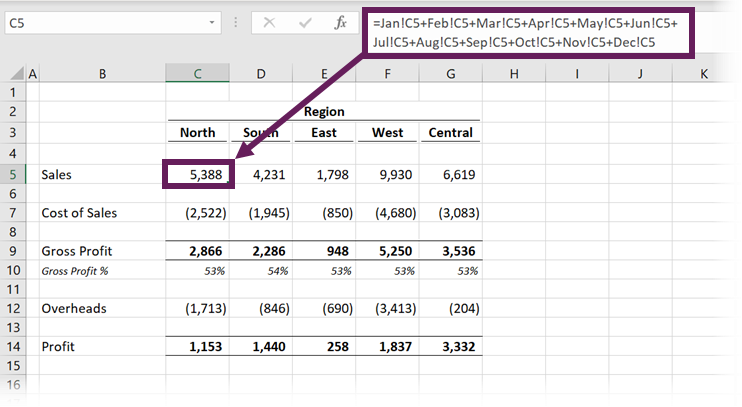
The formula in cell C5 is:
=Jan!C5+Feb!C5+Mar!C5+Apr!C5+May!C5+Jun!C5+
Jul!C5+Aug!C5+Sep!C5+Oct!C5+Nov!C5+Dec!C5
How do you know if you’ve clicked on every worksheet? What if you happened to miss one by accident? There is only one way to know – you’ve got to check it!
The chances are that you don’t need to do all that clicking. And just think about the time you will waste if there is a new tab to be added.
The good news is that there is another approach we can take that will enable us to sum across different sheets easily. I still remember the first time a work colleague showed me this trick; my jaw hit the ground in amazement. I thought he was an Excel genius. That’s why I’m sharing it here; by using this approach, you can look like an Excel genius to your work colleagues too 🙂
To sum the same cell across multiple sheets of a workbook, we can use the following formula structure:
=SUM('FirstSheet:LastSheet'!A1)
- Replace FirstSheet and LastSheet with the worksheet names you wish to sum between. If your worksheet names contain spaces, or are the name of a range (e.g., Q1 could be the name of a sheet or a cell reference ), then single quotes ( ‘ ) are required around the sheet names. If not, the single quotes can be left out.
- Replace A1 with the cell reference you wish to use
With this beautiful little formula, we can see all the worksheets included in the calculation just by looking at the tabs at the bottom. Take a look at the screenshot below. All the tabs from Jan to Dec are included in the calculation.
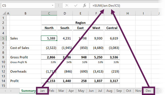
The formula in cell C5 is:
=SUM(Jan:Dec!C5)
SUM across multiple sheets – dynamic
We can change this to be more dynamic, making it even easier to use. Instead of using the names of the first and last tabs, we can create two blank sheets to act as bookends for our calculation.
Take a look at the screenshot below. The Start and End sheets are blank. By dragging sheets in and out of the Start and End bookends, we can sum almost anything we want.
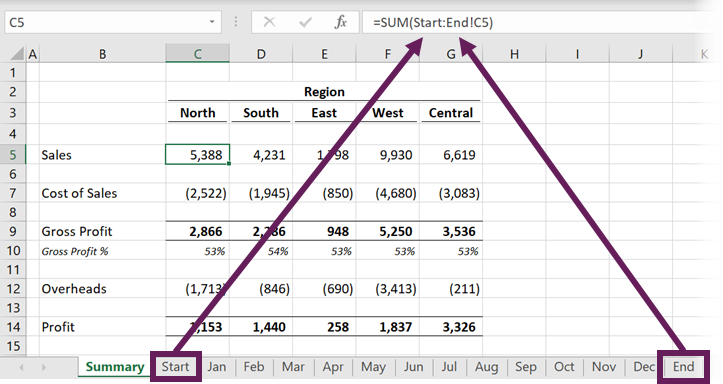
The formula in cell C5 is
=SUM(Start:End!C5)
We can also create sub-calculations. For example, we could add quarters as interim bookends too. There is the added advantage that the tabs also serve as helpful presentation dividers. The example below shows the calculation of just Jan, Feb, and Mar sheets.
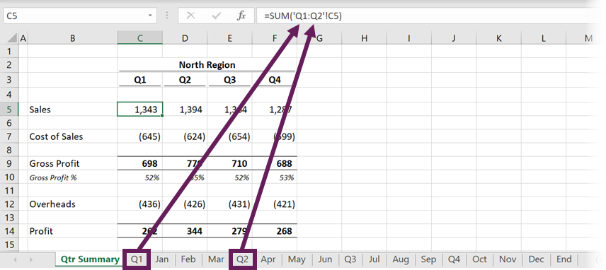
The formula in cell C5 is:
=SUM('Q1:Q2'!C5)
Excel could mistake Q1 and Q2 as cell references; therefore, adding single quotes around the sheet names is essential.
Which other formulas does this work for?
This approach doesn’t just work for the SUM function. Here is a list of all the functions for which this trick works.
| Basic Calculations
SUM AVERAGE AVERAGEA PRODUCT |
Counting
COUNT COUNTA |
Min & Max
MAX MAXA MIN MINA |
Standard deviation
STDEV STDEVA STDEVP STDEVPA |
Variance
VAR VARA VARP VARPA |
The drawbacks
There are a few things to be aware of:
- All the sheets must be in a consistent layout and must stay that way. If one worksheet changes, the formula many not sum the correct cells.
- Usually, formula cell references move automatically when new rows or columns are inserted. This formula does not work like that. It will only move if you select all the sheets and then insert a row or column into all of those sheets at the same time.
- Any sheets which are between the two tabs are included within the calculation. Therefore, even though we cannot see them, hidden sheets are also included in the result.

About the author
Hey, I’m Mark, and I run Excel Off The Grid.
My parents tell me that at the age of 7 I declared I was going to become a qualified accountant. I was either psychic or had no imagination, as that is exactly what happened. However, it wasn’t until I was 35 that my journey really began.
In 2015, I started a new job, for which I was regularly working after 10pm. As a result, I rarely saw my children during the week. So, I started searching for the secrets to automating Excel. I discovered that by building a small number of simple tools, I could combine them together in different ways to automate nearly all my regular tasks. This meant I could work less hours (and I got pay raises!). Today, I teach these techniques to other professionals in our training program so they too can spend less time at work (and more time with their children and doing the things they love).
Do you need help adapting this post to your needs?
I’m guessing the examples in this post don’t exactly match your situation. We all use Excel differently, so it’s impossible to write a post that will meet everybody’s needs. By taking the time to understand the techniques and principles in this post (and elsewhere on this site), you should be able to adapt it to your needs.
But, if you’re still struggling you should:
- Read other blogs, or watch YouTube videos on the same topic. You will benefit much more by discovering your own solutions.
- Ask the ‘Excel Ninja’ in your office. It’s amazing what things other people know.
- Ask a question in a forum like Mr Excel, or the Microsoft Answers Community. Remember, the people on these forums are generally giving their time for free. So take care to craft your question, make sure it’s clear and concise. List all the things you’ve tried, and provide screenshots, code segments and example workbooks.
- Use Excel Rescue, who are my consultancy partner. They help by providing solutions to smaller Excel problems.
What next?
Don’t go yet, there is plenty more to learn on Excel Off The Grid. Check out the latest posts:
See all How-To Articles
This tutorial demonstrates how to count the number of worksheets in an Excel file.
Count Number of Worksheets
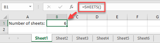
The easiest way to count the number of worksheets in your workbook is to use the SHEETS Function. Say your Excel file has six worksheets.
In any cell on any of the sheets, enter the formula:
=SHEETS()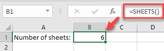
As you can see, this function without arguments returns the total number of sheets in the current workbook (including hidden sheets).
In this article, we will learn how to get the sum or add cells across multiple sheets in Microsoft Excel.
Sometimes we need to access different values from different worksheets of the same excel book. Here we are accessing it to add multiple cells in Excel 2016.
In this article, we will learn how to sum the values located on different sheets in excel 2016. We will use the SUM function to add numbers.
SUM function adds up the values.
SUM = number 1 + number 2 + …
Syntax:
=SUM(number 1, number 2, ..)
Let’s understand how to add cells in excel 2016 with the example explained here.
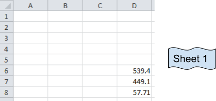
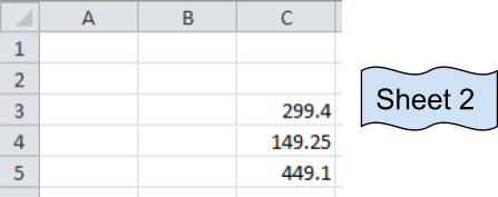
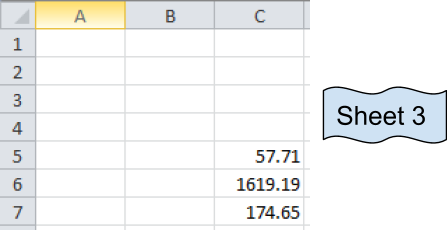
These are numbers from three different sheets and desired output sum will be in Sheet 1.
Now we use the SUM function
Formula:
=SUM(D6:D8, Sheet2!C3:C5,Sheet3!C5:C7)
Explanation:
The resulting output is in Sheet 1.
D6:D8 adds the values of Sheet 1 D6+D7+D8
C3:C5 adds the values of Sheet 2 C3+C4+C5
C5:C7 adds the values of Sheet 3 C5+C6+C7.
It’s basically the addition of values in cells
D6+D7+D8 + C3+C4+C5 + C5+C6+C7
You can select the cells separated by commas to add the numbers.
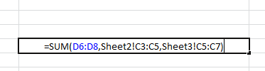
Your formula will look like the above image.
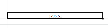
Press Enter and your desired sum will be here in Sheet 1.
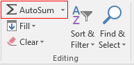
As we can see Sum function returns the sum. You can use Autosum option in Home tab in Editing.
Click arrow key for more options like shown below.
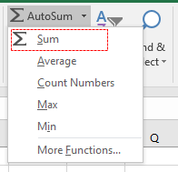
Then select the cells to add up values in Excel. You can sum across the rows and columns using the SUM function.
Hope you got SUM function adding cells in excel. The same function can be performed in Excel 2016, 2013 and 2010. Let us know how you like this article. You will find more content on functions and formulas here. Please state your query down in the comment box. We will help you.
If you liked our blogs, share it with your friends on Facebook. And also you can follow us on Twitter and Facebook. Hope you got SUM function adding cells in excel. The same function can be performed in Excel 2016, 2013 and 2010. Let us know how you like this article. You will find more content on functions and formulas here. Please state your query down in the comment box. We will help you.
We would love to hear from you, do let us know how we can improve, complement or innovate our work and make it better for you. Write us at info@exceltip.com
Popular Articles:
50 Excel Shortcut to Increase Your Productivity
How to use the VLOOKUP Function in Excel
How to use the COUNTIF function in Excel
How to use the SUMIF Function in Excel
Understanding how cells behave in relation to one another is essential to getting the most out of Microsoft Excel. When you’re working with multiple worksheets simultaneously, it can become tedious to click back and forth, manually updating totals. In these instances, it makes sense to set up a totalling worksheet that automatically summarizes data gathered from cells located elsewhere in your workbook.
-
Click the «+» button at the bottom of the Excel screen to insert a new worksheet. This is the worksheet you will use to create your running total. If you want to title the sheet, double-click its tab and enter a title.
-
Add any relevant text labels and formatting to the columns and cells on your new worksheet. If you just want to have one cell displaying a total of a selection of numbers summed up from other worksheets, you might label cell A1 «Running Total,» for example.
-
Click the cell in which you want to display your running total. Following through on the example given in Step 2, you might click cell A2, so that your total displays under your Running Total header.
-
Click your mouse pointer in the formula bar at the top of the screen to initiate Excel’s formula entry capabilities.
-
Enter the following text in the formula bar:
= sum(
-
Click your mouse pointer on the first worksheet tab from which you want to add totalling data, and then click the cell from which you want to gather totalling information. Press the «,» key on your keyboard, and then repeat this step for each of the cells from which you want to gather data for your total.
-
Press the «)» key on your keyboard, and then press «Enter» to finish creating your totalling formula.
After you press Enter, Excel automatically takes you to your totalling worksheet and displays your total in the selected cell. If you click the totalling cell and then look at the formula bar, it should look something like the following:
= SUM(Sheet2!A2,Sheet1!A5)
The «Sheet1» and «Sheet2» values will be replaced by the names of your worksheets, and the «A2» and «A5» values replaced by the cells you clicked in Step 6.