
Total the data in an Excel table
You can quickly total data in an Excel table by enabling the Total Row option, and then use one of several functions that are provided in a drop-down list for each table column. The Total Row default selections use the SUBTOTAL function, which allow you to include or ignore hidden table rows, however you can also use other functions.

-
Click anywhere inside the table.
-
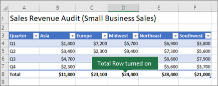
Go to Table Tools > Design, and select the check box for Total Row.

-
The Total Row is inserted at the bottom of your table.
Note: If you apply formulas to a total row, then toggle the total row off and on, Excel will remember your formulas. In the previous example we had already applied the SUM function to the total row. When you apply a total row for the first time, the cells will be empty.
-
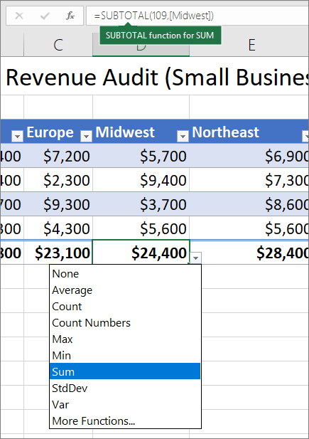
Select the column you want to total, then select an option from the drop-down list. In this case, we applied the SUM function to each column:
You’ll see that Excel created the following formula: =SUBTOTAL(109,[Midwest]). This is a SUBTOTAL function for SUM, and it is also a Structured Reference formula, which is exclusive to Excel tables. Learn more about Using structured references with Excel tables.
You can also apply a different function to the total value, by selecting the More Functions option, or writing your own.
Note: If you want to copy a total row formula to an adjacent cell in the total row, drag the formula across using the fill handle. This will update the column references accordingly and display the correct value. If you copy and paste a formula in the total row, it will not update the column references as you copy across, and will result in inaccurate values.

You can quickly total data in an Excel table by enabling the Total Row option, and then use one of several functions that are provided in a drop-down list for each table column. The Total Row default selections use the SUBTOTAL function, which allow you to include or ignore hidden table rows, however you can also use other functions.
-
Click anywhere inside the table.
-
Go to Table > Total Row.
-
The Total Row is inserted at the bottom of your table.
Note: If you apply formulas to a total row, then toggle the total row off and on, Excel will remember your formulas. In the previous example we had already applied the SUM function to the total row. When you apply a total row for the first time, the cells will be empty.
-
Select the column you want to total, then select an option from the drop-down list. In this case, we applied the SUM function to each column:
You’ll see that Excel created the following formula: =SUBTOTAL(109,[Midwest]). This is a SUBTOTAL function for SUM, and it is also a Structured Reference formula, which is exclusive to Excel tables. Learn more about Using structured references with Excel tables.
You can also apply a different function to the total value, by selecting the More Functions option, or writing your own.
Note: If you want to copy a total row formula to an adjacent cell in the total row, drag the formula across using the fill handle. This will update the column references accordingly and display the correct value. If you copy and paste a formula in the total row, it will not update the column references as you copy across, and will result in inaccurate values.
You can quickly total data in an Excel table by enabling the Toggle Total Row option.
-
Click anywhere inside the table.
-
Click the Table Design tab > Style Options > Total Row.
The Total row is inserted at the bottom of your table.
Set the aggregate function for a Total Row cell
Note: This is one of several beta features, and currently only available to a portion of Office Insiders at this time. We’ll continue to optimize these features over the next several months. When they’re ready, we’ll release them to all Office Insiders, and Microsoft 365 subscribers.
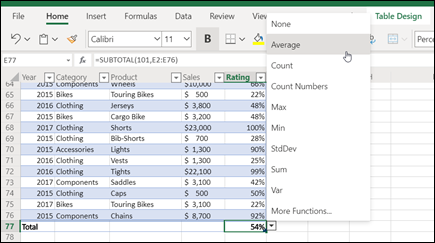
The Totals Row lets you pick which aggregate function to use for each column.
-
Click the cell in the Totals Row under the column you want to adjust, then click the drop-down that appears next to the cell.
-
Select an aggregate function to use for the column. Note that you can click More Functions to see additional options.
Need more help?
You can always ask an expert in the Excel Tech Community or get support in the Answers community.
See Also
Overview of Excel tables
Video: Create an Excel table
Create or delete an Excel table
Format an Excel table
Resize a table by adding or removing rows and columns
Filter data in a range or table
Convert a table to a range
Using structured references with Excel tables
Subtotal and total fields in a PivotTable report
Subtotal and total fields in a PivotTable
Excel table compatibility issues
Export an Excel table to SharePoint
Need more help?
Want more options?
Explore subscription benefits, browse training courses, learn how to secure your device, and more.
Communities help you ask and answer questions, give feedback, and hear from experts with rich knowledge.
Usually, numbers are stored in rows of a single column, so getting the total of those columns is important. However, there are different ways of getting the total. As a beginner, it is important to know the concept of getting the column totals. This article will show you how to get excel totals of columns differently.
Table of contents
- Total Column in Excel
- How to Get Column Total in Excel (with Examples)
- Example #1 – Get Temporary Excel Column Total in Single Click
- Example #2 – Get Auto Column Total in Excel
- Example #3 – Get Excel Column Total by Using SUM Function Manually
- Example #4 – Get Excel Column Total by Using SUBTOTAL Function
- Things to Remember
- Recommended Articles
- How to Get Column Total in Excel (with Examples)
How to Get Column Total in Excel (with Examples)
Here we will show you how to get total columns in Excel with a few examples.
You can download this Column Total Excel Template here – Column Total Excel Template
Example #1 – Get Temporary Excel Column Total in Single Click
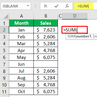
If you need a quick total of the column and see the total of any column, then this option will show a quick sum of numbers in the column.
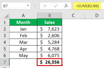
- For example, look at the below data in Excel.
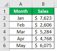
- To get the total of this column “B,” select the entire column or the data range from B2 to B6. Then, we need to select the whole column and see the “Status Bar.”
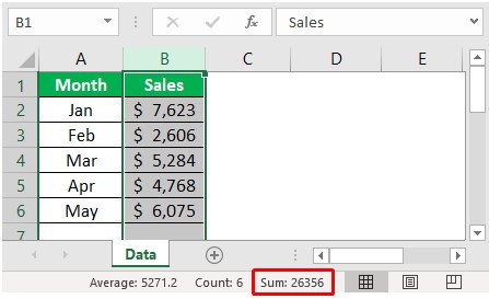
As we can see in the status barAs the name implies, the status bar displays the current status in the bottom right corner of Excel; it is a customizable bar that can be customized to meet the needs of the user.read more, we have a quick sum showing as 26,356.
- Instead of selecting the entire column, we must choose the only data range and see the result.
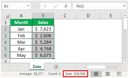
The total is the same, but the only difference is the formatting of numbers. In the previous case, we selected the entire column, and the formatting of numbers was not there. But this time, since we have chosen only the numbers range in the quick sum, too. So then, we can see the same formatting of the selected range.
Example #2 – Get Auto Column Total in Excel
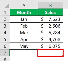
The temporary total can be seen to make the calculations permanently visible in a cell. We can use the autosum option. For example, in the above data, we have data till the 6th row, so in the 7th row, we need the total of the above column numbers.
- We must select the cell which is just below the last data cell.
- Now press the “ALT + =” shortcut key to insert the AUTOSUM option.
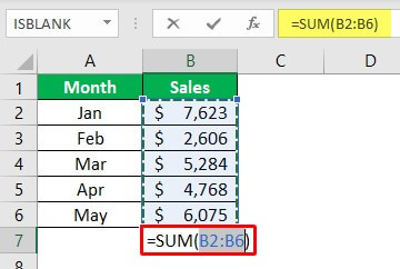
- As we can see above, it has automatically inserted the SUM function in excelThe SUM function in excel adds the numerical values in a range of cells. Being categorized under the Math and Trigonometry function, it is entered by typing “=SUM” followed by the values to be summed. The values supplied to the function can be numbers, cell references or ranges.read more upon pressing the shortcut key “ALT + =” and pressing the “Enter” key to get the column total.
Since we have selected only the data range, it has given us the same formatting of the selected cells.
- However, there are certain limitations to this AUTOSUM function, especially when we work with a large number of cells. Now, look at the below data.
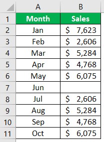
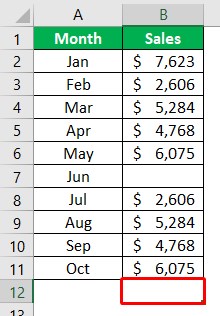
- In the above data, we have data range till the 11th row. So in the 12th row, we need the column total, so select cell B12.
- After that, we need to press the ALT + = sign shortcut key to insert the quick SUM function.
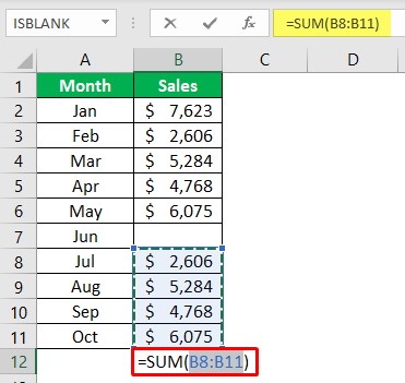
Look at the limitation of the AUTOSUM function. It has selected only four cells above. After the 4th cell, we have a blank cell, so the AUTOSUM shortcut thinks this will be the end of the data and returns only four cells summation.
In this case, this is a small sample size, but when the data is larger, it may go unnoticed. That is where we need to use the manual SUM function.
Example #3 – Get Excel Column Total by Using SUM Function Manually
- We can open the SUM function in any cell other than the column of numbers.
- For the SUM function, choose the entire column of “B.”
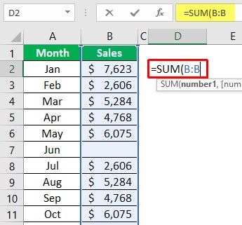
- Then, close the bracket and press the “Enter” key to get the result.

So this will take the entire column into consideration and display results accordingly. Since the whole column has been selected, we need not worry about the missing cells.
Example #4 – Get Excel Column Total by Using SUBTOTAL Function
The SUBTOTAL function in excelThe SUBTOTAL excel function performs different arithmetic operations like average, product, sum, standard deviation, variance etc., on a defined range.read more is very powerful to show only displayed cell results.
- We must open the SUBTOTAL function first.

- Upon opening the SUBTOTAL function, we have many kinds of calculation types. From the list, choose the 9-SUM function.

- Next, choose the above range of cells.

- Then, close the bracket and press the “Enter key” to get the result.
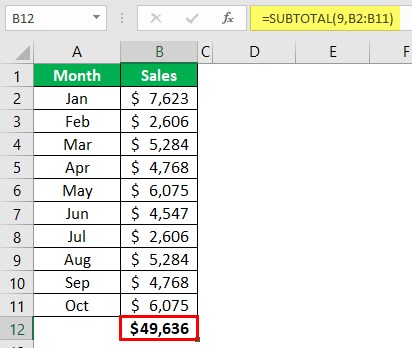
We have got the total of the column. But the question is, if the SUM function returned the same, then what is the point of using SUBTOTAL.
- The special thing is that SUBTOTAL displays the calculation only for visible cells. So, for example, apply a filter and choose only any of the three months.
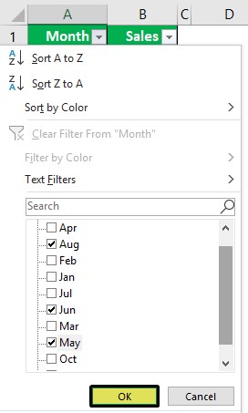
- We have chosen only the “Aug, Jun, and May” months. Then, click on “OK” and see the result.

The result of a SUBTOTAL function is limited to only visible cells, not the entire range of cells, so this is the specialty of the SUBTOTAL function.
Things to Remember
- The AUTOSUM takes the only reference of non-empty cells, and at the finding of empty cells, it will stop its reference.
- If any minus value is between, all those values will be deducted, and the result is the same as the mathematical rule.
Recommended Articles
This article has been a guide to Excel Column Total. We learn how to get a column total in Excel using the SUM and SUBTOTAL function and examples and a downloadable Excel template. You may learn more about Excel from the following articles: –
- SUM Shortcut in Excel
- How to Sum by Color in Excel?
- SUMIF Function in Excel
- Themes in Excel
Asked by: Augusta Ruecker
Score: 5/5
(41 votes)
Select a cell next to the numbers you want to sum, click AutoSum on the Home tab, press Enter, and you’re done. When you click AutoSum, Excel automatically enters a formula (that uses the SUM function) to sum the numbers.
How do I total a SUM in Excel?
To sum a range of cells, use the SUM function. To sum cells based on one criteria (for example, greater than 9), use the following SUMIF function (two arguments). To sum cells based on one criteria (for example, green), use the following SUMIF function (three arguments, last argument is the range to sum).
What is the formula for SUM in Excel?
The SUM function adds values. You can add individual values, cell references or ranges or a mix of all three. For example: =SUM(A2:A10) Adds the values in cells A2:10.
How do you total a row in Excel?
You can quickly total data in an Excel table by enabling the Toggle Total Row option.
- Click anywhere inside the table.
- Click the Table Design tab > Style Options > Total Row. The Total row is inserted at the bottom of your table.
How do I enable filtering?
Try it!
- Select any cell within the range.
- Select Data > Filter.
- Select the column header arrow .
- Select Text Filters or Number Filters, and then select a comparison, like Between.
- Enter the filter criteria and select OK.
22 related questions found
How do you create a formula for a column in Excel?
To insert a formula in Excel for an entire column of your spreadsheet, enter the formula into the topmost cell of your desired column and press «Enter.» Then, highlight and double-click the bottom-right corner of this cell to copy the formula into every cell below it in the column.
What is Excel average formula?
Description. Returns the average (arithmetic mean) of the arguments. For example, if the range A1:A20 contains numbers, the formula =AVERAGE(A1:A20) returns the average of those numbers.
How many Excel formulas are there?
Excel has over 475 formulas in its Functions Library, from simple mathematics to very complex statistical, logical, and engineering tasks such as IF statements (one of our perennial favorite stories); AND, OR, NOT functions; COUNT, AVERAGE, and MIN/MAX.
Which formula is not entered correctly?
Solution(By Examveda Team)
A formula always starts with an equal sign (=), which can be followed by numbers, math operators (such as a plus or minus sign), and functions, which can really expand the power of a formula. Here in option D 10+50 there is no equal sign (=), so it is not correct.
What is count A in Excel?
Description. The COUNTA function counts the number of cells that are not empty in a range.
Is there a Sumif function in Excel?
The Excel SUMIF function returns the sum of cells that meet a single condition. Criteria can be applied to dates, numbers, and text. The SUMIF function supports logical operators (>,<,<>,=) and wildcards (*,?) for partial matching.
How do you create spreadsheet?
Open a new, blank workbook
- Click the File tab.
- Click New.
- Under Available Templates, double-click Blank Workbook. Keyboard shortcut To quickly create a new, blank workbook, you can also press CTRL+N.
Which symbol is entered before a formula?
If you type in the formula, you must start with an equal sign, so Excel knows that the data in the cell is a formula. After the =, what comes next depends on what you’re trying to do. If you are multiplying numbers, just type in the appropriate numbers and mathematical symbol (* for multiply).
Which is not a function in MS Excel?
The correct answer to the question “Which one is not a function in MS Excel” is option (b). AVG. There is no function in Excel like AVG, at the time of writing, but if you mean Average, then the syntax for it is also AVERAGE and not AVG. The other two options are correct.
How can u activate a cell?
Answer: D. A cell can be ready to activate by any of the method Pressing the Tab key or Clicking the cell or Pressing an arrow key.
What are the 5 functions in Excel?
To help you get started, here are 5 important Excel functions you should learn today.
- The SUM Function. The sum function is the most used function when it comes to computing data on Excel. …
- The TEXT Function. …
- The VLOOKUP Function. …
- The AVERAGE Function. …
- The CONCATENATE Function.
What is basic formula?
Formula is an expression that calculates values in a cell or in a range of cells. For example, =A2+A2+A3+A4 is a formula that adds up the values in cells A2 through A4. Function is a predefined formula already available in Excel.
What are the top 10 Excel formulas?
Top 10 Most Useful Excel Formulas
- SUM, COUNT, AVERAGE. SUM allows you to sum any number of columns or rows by selecting them or typing them in, for example, =SUM(A1:A8) would sum all values in between A1 and A8 and so on. …
- IF STATEMENTS.
- SUMIF, COUNTIF, AVERAGEIF.
- VLOOKUP. …
- CONCATENATE. …
- MAX & MIN. …
- AND. …
- PROPER.
What is grade formula Excel?
To find the grade, multiply the grade for each assignment against the weight, and then add these totals all up. … So for each cell (in the Total column) we will enter =SUM(Grade Cell * Weight Cell), so my first formula is =SUM(B2*C2), the next one would be =SUM(B3*C3) and so on.
What is Max function in Excel?
The Excel MAX function returns the largest numeric value in a range of values. The MAX function ignores empty cells, the logical values TRUE and FALSE, and text values. Get the largest value. The largest value in the array.
How do I automatically apply formulas in Excel without dragging?
Simply do the following:
- Select the cell with the formula and the adjacent cells you want to fill.
- Click Home > Fill, and choose either Down, Right, Up, or Left. Keyboard shortcut: You can also press Ctrl+D to fill the formula down in a column, or Ctrl+R to fill the formula to the right in a row.
How do I add a formula to existing data in Excel?
Just select all the cells at the same time, then enter the formula normally as you would for the first cell. Then, when you’re done, instead of pressing Enter, press Control + Enter. Excel will add the same formula to all cells in the selection, adjusting references as needed.
How do I do a percentage formula in Excel?
The percentage formula in Excel is = Numerator/Denominator (used without multiplication by 100). To convert the output to a percentage, either press “Ctrl+Shift+%” or click “%” on the Home tab’s “number” group.
Can you start a formula in Excel with?
Simple formulas always start with an equal sign (=), followed by constants that are numeric values and calculation operators such as plus (+), minus (-), asterisk(*), or forward slash (/) signs. Let’s take an example of a simple formula. On the worksheet, click the cell in which you want to enter the formula.
Running total (also called cumulative sum) is quite commonly used in many situations. It’s a metric that tells you what’s the sum of the values so far.
For example, if you have the monthly sales data, then a running total would tell you how much sales have been done till a specific day from the first day of the month.
There are also some other situations where running total is often used, such as calculating your cash balance in your bank statements/ledger, counting calories in your meal plan, etc.
In Microsoft Excel, there are multiple different ways to calculate running totals.
The method you choose would also depend on how your data is structured.
For example, if you have simple tabular data then you can use a simple SUM formula, but if you have an Excel table, then it’s best to use structured references. You can also use Power Query to do this.
In this tutorial, I’m going to cover all these different methods to calculate running totals in Excel.
So let’s get started!
Calculating Running Total with Tabular Data
If you have tabular data (i.e., a table in Excel which is not converted into an Excel table), you can use some simple formulas to calculate the running totals.
Using the Addition Operator
Suppose you have date-wise sales data and you want to calculate the running total in column C.

Below are the steps to do this.
Step 1 – In cell C2, which is the first cell where you want the running total, enter
=B2
This will simply get the same sale values in cell B2.

Step 2 – In cell C3, enter the below formula:
=C2+B3

Step 3 – Apply the formula to the entire column. You can use the Fill handle to select and drag it, or simply and copy-paste the cell C3 to all the remaining cells (which would automatically adjust the reference and give the right result).
This will give you the result as shown below.

It’s a really simple method and works well in most cases.
The logic is simple – every cell picks up the value above it (which is the cumulative sum till the date before) and adds the value in the cell adjacent to it (which is the sale value for that day).
There is only one drawback – in case you delete any of the existing rows in this data set, all the cells below that would return a reference error (#REF!)

If that’s a possibility with your data set, use the next method that uses the SUM formula
Using SUM with Partially Locked Cell Reference
Suppose you have date-wise sales data and you want to calculate the running total in column C.
Below is the SUM formula that will give you the running total.
=SUM($B$2:B2)

Let me explain how this formula works.
In the above SUM formula, I have used the reference to add as $B$2:B2
- $B$2 – this is an absolute reference, which means that when I copy the same formula in the cells below, this reference is not going to change. So when copying the formula in the cell below, the formula would change to SUM($B$2:B3)
- B2 – this is the second part of the reference which is a relative reference, which means that this would adjust as I copy the formula down or to the right. So when copying the formula in the cell below, this value will become B3
Also read: Absolute, Relative, and Mixed Cell References in Excel
The great thing about this method is that in case you delete any of the rows in the data set, this formula would adjust and still give you the right running totals.
Calculating Running Total in Excel Table
When working with tabular data in Excel it’s a good idea to convert it into an Excel table. It makes it a lot easier to manage the data and also allows makes it easy to use tools such as Power Query and Power Pivot.
Working the Excel tables comes with benefits such as structured references (which makes it really easy to refer to the data in the table and use it in formulas), and automatic adjustment of references in case you add or delete data from the table.
While you can still use the above formula that I have shown you in an Excel table, let me show you some better methods to do this.
Suppose you have an Excel table as shown below and you want to calculate the running total in column C.

Below is the formula that will do this:
=SUM(SalesData[[#Headers],[Sale]]:[@Sale])

The above formula may look a bit long, but you don’t have to write it yourself. what you see within the sum formula are called structured references, which is Excel’s efficient way to refer to specific data points in an Excel table.
For example, SalesData[[#Headers],[Sale]] refers to the Sale header in the SalesData table (SalesData is the name of the Excel table that I gave when I created the table)
And [@Sale] refers to the value in the cell in the same row in the Sale column.
I just explained this here for your understanding, but even if you know nothing about structured references, you can still easily create this formula.
Below are the steps to do this:
- In cell C2, enter =SUM(
- Select cell B1, which is the header of the column that has the sale value. You can use the mouse or use the arrow keys. You will notice that Excel automatically enters the structured reference for that cell
- Add a : (colon symbol)
- Select cell B2. Excel would again automatically insert the structured reference for the cell
- Close the bracket and hit enter
You will also notice that you don’t have to copy the formula in the entire column, an Excel table automatically does it for you.
Another great thing about this method is that in case you add a new record in this data set, the Excel table would automatically calculate the running total for all the new records.
While we have included the header of the column in our formula, remember that the formula would ignore the header text and only consider the data in the column
Calculating Running Total Using Power Query
Power Query is an amazing tool when it comes to connecting with databases, extracting the data from multiple sources, and transforming it before putting it into Excel.
If you are already working with Power Query, it would be more efficient to add running totals while you are transforming the data within the Power Query editor itself (instead of 1st getting the data in Excel and then adding the running totals using any of the above methods covered above).
While there is no inbuilt feature in Power Query to add running totals (which I wish there was), you can still do that using a simple formula.
Suppose you have an Excel table as shown below and you want to add the running totals to this data:

Below are the steps to do this:
- Select any cell in the Excel table
- Click on Data

- In the Get & Transform tab, click on the from Table/Range icon. This will open the table in the Power Query editor
- [Optional] In case your Date column is not already sorted, click on the filter icon in the Date column, and then click on Sort ascending

- Click the Add Column tab in the Power Query editor

- In the General group, click on the Index Column dropdown (do not click on the Index Column icon, but on the small black tilted arrow right next to it to show more options)
- Click on the ‘From 1’ option. Doing this will add a new index column that would start from one and enter numbers incrementing by 1 in the entire column

- Click on the ‘Custom Column’ icon (which is also in the Add Column tab)

- In the custom column dialog box that opens up, enter a name for the new column. in this example, I will use the name ‘Running Total’

- In the Custom column formula field, enter the below formula: List.Sum(List.Range(#”Added Index”[Sale],0,[Index]))

- Make sure there’s a checkbox at the bottom of the dialog box that says – ‘No syntax errors have been detected’
- Click OK. This would add a new running total column
- Remove the Index Column

- Click on the File tab and then click on ‘Close and Load’


The above steps would insert a new sheet in your workbook with a table that has the running totals.

Now if you’re thinking that these are just too many steps as compared to the previous methods of using simple formulas, you’re right.
If you already have a data set and all you need to do is add running totals, it’s better not to use Power Query.
Using Power Query makes sense where you have to extract data from a database or combine data from multiple different workbooks and in the process also add running totals to it.
Also, once you do this automation using Power Query, the next time your data set changes you do not have to do it again you can simply refresh the query and it would give you the result based on the new data set.
How does this work?
Now let me quickly explain what happens in this method.
The first thing we do in the Power Query editor is to insert an index column starting from one and incrementing by one as it goes down the cells.
We do this because we need to use this column while we calculate the running total in another column that we insert in the next step.
Then we insert a custom column and use the below formula
List.Sum(List.Range(#"Added Index"[Sale],0,[Index]))
This is a List.Sum formula that would give you the sum of the range that is specified within it.
And that range is specified using the List.Range function.
The List.Range function gives the specified range in the sale column as the output and this range changes based on the Index value. For example, for the first record, the range would simply be the first sale value. And as you go down the cells, this range would expand.
So, for the first cell. List.Sum would only give you the sum of the first sale value, and for the second cell, it would give you the sum for the first two sale values and so on.
While this method works well, gets really slow with large datasets – thousands of rows. If you’re dealing with a large data set and want to add running totals to it, have a look at this tutorial that shows other methods that are faster.
Calculating Running Total Based on Criteria
So far, we have seen examples where we have calculated the running total for all the values in a column.
But there could be cases where you want to calculate the running total for specific records.
For example, below I have a data set and I want to calculate the running total for Printers and Scanners separately in two different columns.

This can be done using a SUMIF formula that calculates the running total while making sure the specified condition is met.
Below is the formula that will do this for the Printer columns:
=SUMIF($C$2:C2,$D$1,$B$2:B2)

Similarly, to calculate the running total for Scanners, use the below formula:
=SUMIF($C$2:C2,$E$1,$B$2:B2)

In the above formulas, I have used SUMIF, which would give me the sum in a range when the specified criteria are met.
The formula takes three arguments:
- range: this is the criteria range that would be checked against the specified criteria
- criteria: this is the criteria that would be checked in only if this criterion is met then the values in the third argument, which is the sum range, would be added
- [sum_range]: this is the sum range from which the values would be added if the criteria are met
Also, in the range and sum_range argument, I have locked the second part of the reference, so that as we go down the cells, the range would keep expanding. This allows us to only consider and add values till that range (hence running totals).
In this formula, I have used the header column (Printer and Scanner) as the criteria. you can also hardcode the criteria if your column headers are not exactly the same as the criteria text.
In case you have multiple conditions that you need to check, then you can use the SUMIFS formula.
Running Total in Pivot Tables
If you want to add running totals in a Pivot Table result, you can easily do that using an inbuilt functionality in Pivot tables.
Suppose you have a Pivot Table as shown below where I have the date in one column and the sale value in the other column.

Below are the steps to add an additional column that will show the running total of the sales by date:
- Drag the Sale field and put it in the Value area.

- This will add another column with the Sales values
- Click on the Sum of Sale2 option in the Value area
- Click on the ‘Value Field Settings’ option

- In the Value Field Settings dialog box, change the Custom Name to ‘Running Totals’

- Click on the ‘Show Value As’ tab
- In the Show value as drop-down, select the ‘Running Total in’ option
- In the Base field options, make sure Date is selected
- Click Ok


The above steps would change the second sale column into the Running Total column.

So these are some of the ways you can use to calculate the running total in Excel. If you have data in tabular format, you can use simple formulas, and if you have an Excel table, then you can use formulas that make use of structured references.
I’ve also covered how to calculate running total using Power Query and in Pivot Tables.
I hope you found this tutorial useful.
Other Excel tutorials you may also like:
- How to Sum a Column in Excel
- Calculating Moving Average in Excel [Simple, Weighted, & Exponential]
- Excel Quick Analysis Tool – How to Best Use it? 10 Examples!
Tables are one of the best features of Excel. While it is possible to use the standard cell referencing with a Table, they have their own referencing style called structured references. We have to think a little differently to create a running total in an Excel Table using structured references.
We will look at all the options in this post.
Download the example file
I recommend you download the example file for this post. Then you’ll be able to work along with examples and see the solution in action, plus the file will be helpful for future reference.
![]()
Download the file: 0075Running Totals in Excel Tables.zip
Watch the video
Watch the video on YouTube.
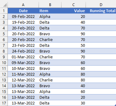
The example
All the scenarios in this post use the same Table. The goal is to:
- Create a running total in the Running Total column
- Ensure values calculate correctly when rows are added or deleted
Normal cell references
We could use normal cell references in either the A1 or R1C1 style. For this, there are two common options (1) Cell above + value (2) Expanding range with mixed references.
Method #1: Cell above + value
The purpose of a Table is to use the same formula in each row of the column. Therefore, it is not possible to just use the cell above plus the value method.
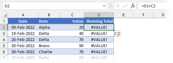
The formula in Cell D2 is:
=D1+C2
The result of the formula is #VALUE!; Cell D1 is a text value, which cannot be added to a number using a basic calculation.
However, the SUM function ignores text values; therefore, by using SUM with a comma (known as the Union Operator), the text value will be calculated as a zero. This avoids the #VALUE! error.
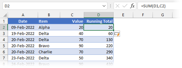
The formula in Cell D2 is:
=SUM(D1,C2)
The result of this formula is a running total in each row of the Running Total column.
Rather than SUM, you could also use the N function. This returns zero if the cell reference within it is not a number; otherwise, it returns the number. For example, if Cell D2 contained the following formula, it would also create a running total.
=N(D1)+C2
However, both methods all fall short when rows are deleted. The screenshot below shows the result after Row 4 has been deleted.
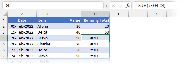
As you can see by the #REF! error, this method does not work when rows are deleted. This does not meet the requirements we wanted.
Method #2: Expanding range with mixed references
There is another method we can take using standard ranges that uses mixed references.
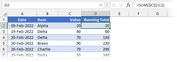
The formula in Cell D2 is:
=SUM($C$2:C2))
This method creates an expanding range for each row in the Table.
So, if you delete a row, it still works… perfect! Or is it? The problem comes when you add a new row of data to the bottom:
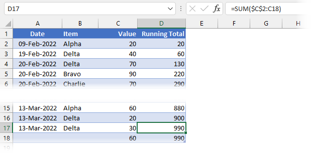
There isn’t an obvious problem at the start. But, take a look at cell D17; what is the formula that has been automatically copied down? The formula references cell C18 (the last row of the Table), which is incorrect.
=SUM($C$2:C18)
Using this method, adding rows causes the formulas to expand to include the last row, which creates a calculation issue. Therefore, this isn’t a suitable method either.
Structured references
We really want to use structured references. After all, that is the whole point of using a Table.
Method #3: SUM with header row
In the previous section, we identified that SUM ignores text values. Given that the header row in a Table is always text and an absolute row reference (i.e., it doesn’t move when a cell is dragged down), we can create a running total with just the SUM function and structured references.
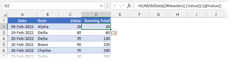
The formula in Cell D2 is:
=SUM(tblData[[#Headers],[Value]]:[@Value])
The result of this formula is a running total in each row.
- tblData[[#Headers],[Value]] is the reference to the header row
- [@Value] is the reference to the cell within the Value column contained on the same row
- : (Colon) between two cell references creates a range
It is easier to see this method at work when we select a cell from the Running Total column.
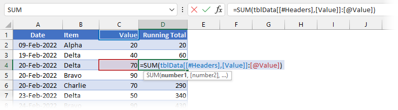
Even though the entire range is not shown, a single range is created between the blue and red boxes.
We can delete or add to the Table, and it still works. AMAZING!
This appears to be the perfect method. However, I feel that using the header row makes this more of a visual solution than a data solution. By which I mean, in other parts of Excel, such as Power Query and Power Pivot, it’s not possible to reference the value in a header row. Therefore, this only works because the data is contained on an Excel worksheet.
I know this works, but conceptually, I feel we should look for another solution.
Method #4: INDEX function
All is not lost; there is another method.
The INDEX function makes it possible to reference any cell within a column.
=INDEX([Value],1)
Therefore, rather than using the column header cell, we can create an absolute reference by selecting the first cell in the column using the INDEX function.
Look at the solution below:
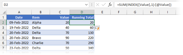
The formula in Cell D2 is:
=SUM(INDEX([Value],1):[@Value])
- INDEX([Value],1) is always a reference to the first cell in the Value column
- [@Value] is the reference to the cell within the Value column contained on the same row
- : (Colon) between the two cell references creates a range
The result of this formula is a non-volatile running total in each row of the Running Total column. It calculates correctly even if rows are added or deleted.
Perfect! This is my preferred option.
Other options
There are other options using OFFSET and relative named ranges that we could use. However, I have discounted these because:
- OFFSET is a volatile function that recalculates every time a cell changes in Excel, which can cause slow spreadsheet calculation times.
- Relative named ranges are a technique to use when you’re stuck or backed into a corner. However, we have suitable techniques without resorting to this.
Running total with criteria
Let’s suggest that we don’t want a single running total, but the running total for each individual element in the Item column. Can our INDEX method handle that situation? You bet it can.
Method #5: INDEX with SUMIFS
We will use the same INDEX technique inside the SUMIFS function.
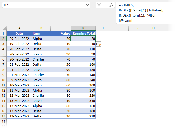
The formula in Cell D2 is:
=SUMIFS(INDEX([Value],1):[@Value],INDEX([Item],1):[@Item],[@Item])
You will notice this uses the same INDEX method as above to create a dynamic range inside both the sum_range and criteria_range1 arguments of the SUMIFS function.
Let’s check this works:
- Alpha exists in Cells B2 (20) and B12 (80). The value in Cell C12 should therefore be 100, which it is. ✅
- Alpha also exists in Cell B15 (60). The value in Cell C15 should be 160, which it is.✅
This method works when rows and added or deleted, precisely what we need. See, the INDEX method is very flexible.
Conclusion
There you have it, lots of options to achieve a running total in an Excel Table. But, there are also lots of pitfalls.
The methods using standard references cannot guarantee the correct values when adding or deleting rows, so these should be discounted.
Both structured referencing methods can be used with COUNT, COUNTIFS, MIN, MINIFS, MAX, MAXIFS, AVERAGE, and AVERAGEIFS.
The SUM + header row method works, but conceptually, I have an issue with referencing the header row in this way. Don’t get me wrong; if it were the only option, I would definitely use it.
The SUM + INDEX method is my preferred choice. It’s flexible and provides everything we need.

About the author
Hey, I’m Mark, and I run Excel Off The Grid.
My parents tell me that at the age of 7 I declared I was going to become a qualified accountant. I was either psychic or had no imagination, as that is exactly what happened. However, it wasn’t until I was 35 that my journey really began.
In 2015, I started a new job, for which I was regularly working after 10pm. As a result, I rarely saw my children during the week. So, I started searching for the secrets to automating Excel. I discovered that by building a small number of simple tools, I could combine them together in different ways to automate nearly all my regular tasks. This meant I could work less hours (and I got pay raises!). Today, I teach these techniques to other professionals in our training program so they too can spend less time at work (and more time with their children and doing the things they love).
Do you need help adapting this post to your needs?
I’m guessing the examples in this post don’t exactly match your situation. We all use Excel differently, so it’s impossible to write a post that will meet everybody’s needs. By taking the time to understand the techniques and principles in this post (and elsewhere on this site), you should be able to adapt it to your needs.
But, if you’re still struggling you should:
- Read other blogs, or watch YouTube videos on the same topic. You will benefit much more by discovering your own solutions.
- Ask the ‘Excel Ninja’ in your office. It’s amazing what things other people know.
- Ask a question in a forum like Mr Excel, or the Microsoft Answers Community. Remember, the people on these forums are generally giving their time for free. So take care to craft your question, make sure it’s clear and concise. List all the things you’ve tried, and provide screenshots, code segments and example workbooks.
- Use Excel Rescue, who are my consultancy partner. They help by providing solutions to smaller Excel problems.
What next?
Don’t go yet, there is plenty more to learn on Excel Off The Grid. Check out the latest posts: