
Count Names in Excel (Table of Contents)
- Overview of Count Names in Excel
- How to Count Names in Excel?
Overview of Count Names in Excel
COUNT is an in-built function in MS Excel that will count the number of cells that contain numbers. It comes under the statistical function category and is used to return an integer as output. There are many ways to count the cells in the given range with several user criteria. Examples are COUNTIF, DCOUNT, COUNTA, etc.
Formula: There are many value parameters in the simple count function, which will count all cells which contain numbers.
There are some specific in-built Count functions which are listed below:
- COUNT: It will count the number of cells that contain the numbers.
- COUNTIF: It will count the number of cells containing the numbers and satisfy the user’s criteria.
- DCOUNT: It will count the cells containing some number in the selected database and satisfy the user criteria.
- DCOUNTA: It will count the non-blank cells in the selected database which satisfy the user criteria.
How to Count Names in Excel?
Counting Names in excel is very simple and easy. So, here are some examples that can help you to Count Names in Excel.
You can download this Count Names Excel Template here – Count Names Excel Template
Example #1 – Count Name which has Age Data
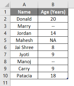
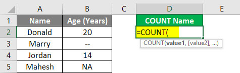
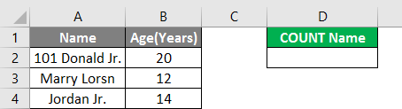
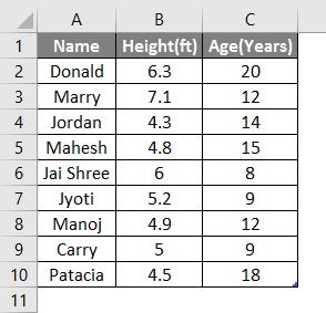
Let’s assume a user has some people’s data like Name and Age, where the user wants to calculate the count of the name with age data in the table.
Let’s see how we can do this with the count function.
Step 1: Open MS Excel from the start menu >> Go to Sheet1, where the user keeps the data.
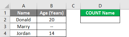
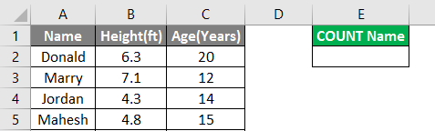
Step 2: Now create headers for the Count name where the user wants the count name, which has age data.
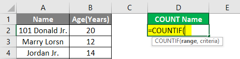
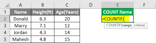
Step 3: Now calculate the count of a name in the given data by the Count function>> use the equal sign to calculate >> Write in D2 Cell and use COUNT>> “=COUNT (”
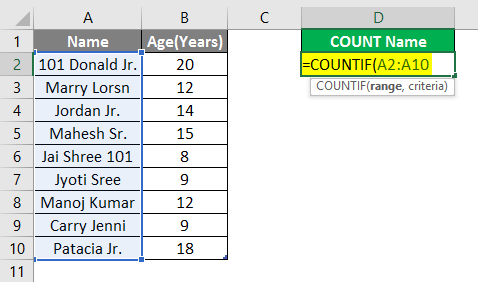
Step 4: Now, it will ask for the value1 which are given in B2 to B10 cell >> select B2 to B10 cell >> “=COUNT (B2: A10)”
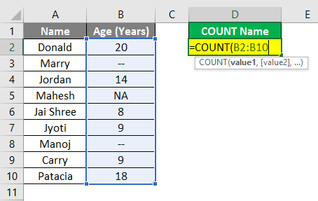
Step 5: Now press the Enter key.
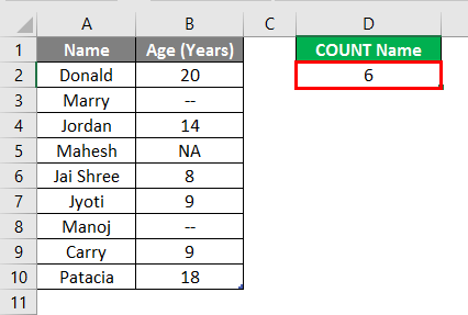
Summary of Example #1: The user wants to calculate the name count, which has age data in the table. So, 6 names in the above example have age data in the table.
Example #2 – Count Name which has Some Common String
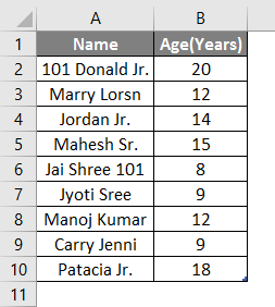
Let’s assume a user has some people’s personal data like Name and Age, where the user wants to calculate the count of the name with the “Jr.” string common in their name. Let’s see how we can do this with the COUNTIF function.
Step 1: Open MS Excel from the start menu >> Go to Sheet2, where the user keeps the data.
Step 2: Create a header for the Count name, with a “Jr.” string common in their name.
Step 3: Now calculate the count of a name in the given data by the COUNTIF function>> use the equal sign to calculate >> Write in D2 Cell and use COUNTIF>> “=COUNTIF (”
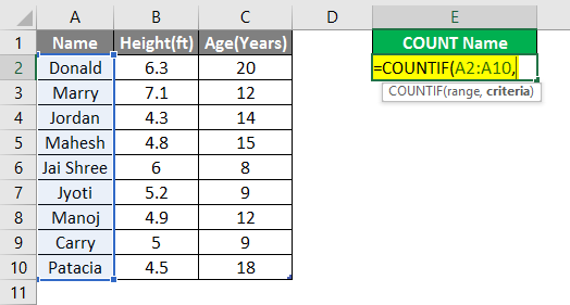
Step 4: Now, it will ask for value1 which are given in A2 to A10 cell >> select A2 to A10 cell >> “=COUNTIF (A2: A10,”
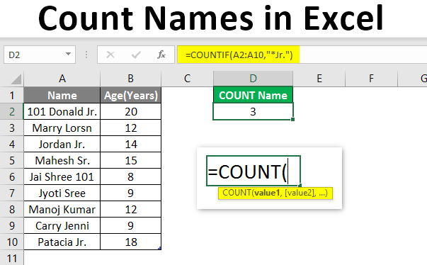
Step 5: Now it will ask for criteria which are to search only for the “Jr.” string in the name >>so write in D2 cell >> “=COUNTIF (A2: A10,” *Jr.”)”
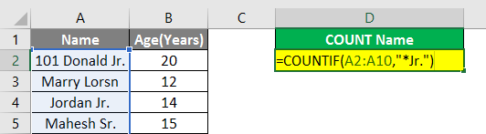
Step 6: Now press the Enter key.

Summary of Example #2: The user wants to count the name with the “Jr.” string common in their name in the table. So, three names in the above example have the “Jr.” string in their name.
Example #3 – Number of Letters with Ending a Specific String
Let’s assume a user wants to count the names with 5 letters and the “ry” string common in their name. Let’s see how we can do this with the COUNTIF function.
Step 1: Open MS Excel from the start menu >> Go to Sheet3, where the user keeps the data.
Step 2: Create a header for the Count name, with 5 letters and a “ry” string common in their name.
Step 3: Now calculate the count of a name in the given data by the COUNTIF function>> use the equal sign to calculate >> Write in E2 Cell and use COUNTIF>> “=COUNTIF (”
Step 4: Now, it will ask for value1 which are given in A2 to A10 cell >> select A2 to A10 cell >> “=COUNTIF (A2: A10,”
Step 5: Now it will ask for criteria which are to search only for the “ry” string in the name with 5 letters>>so write in E2 cell >> “=COUNTIF (A2: A10,”???ry”)”
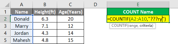
Step 6: Now press the Enter key.
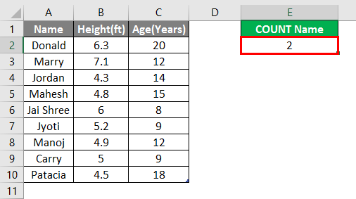
Summary of Example #3: The user wants to count the names with 5 letters in the Name and the “ry” string common in their name in the table. So, 2 names in the above example have a “ry” string in their name with five letters.
Things to Remember About Count Names in Excel
- The Count function comes under the statistical function category and is used to return an integer as output.
- If a cell contains any value that is not numeric, like text or #NA, it will not be counted by the count function.
- The asterisk (*) matches any set of characters in the COUNTIF criteria.
- The question mark (?) is used as the wildcard character to match any single character in the criteria of the function.
- In the criteria, a user can use greater than “>,” less than “<” or equal to the “=” symbol to create criteria in the function. As an example, “=COUNTIF (A2:A5,” >=10″)” here as the output will return the count of the cell, which has a value greater than or equal to 10.
Recommended Articles
This is a guide to Count Names in Excel. Here we discuss How to Count Names in Excel, examples, and a downloadable excel template. You may also look at the following articles to learn more –
- Count Cells with Text in Excel
- Count Characters in Excel
- Count Formula in Excel
- COUNTIFS in Excel
You can use the following methods to count names in Excel:
Method 1: Count Cells with Exact Name
=COUNTIF(A2:A11, "Bob Johnson")
Method 2: Count Cells with Partial Name
=COUNTIF(A2:A11, "*Johnson*")
Method 3: Count Cells with One of Several Names
=COUNTIF(A2:A11, "*Johnson*") + COUNTIF(A2:A11, "*Smith*")
The following examples show how to use each method with the following dataset in Excel:

Example 1: Count Cells with Exact Name
We can use the following formula to count the number of cells in column A that contain the exact name “Bob Johnson”:
=COUNTIF(A2:A11, "Bob Johnson")
The following screenshot shows how to use this formula in practice:

We can see that there are 2 cells that contain “Bob Johnson” as the exact name.
Example 2: Count Cells with Partial Name
We can use the following formula to count the number of cells in column A that contain “Johnson” anywhere in the name:
=COUNTIF(A2:A11, "*Johnson*")
The following screenshot shows how to use this formula in practice:

We can see that there are 4 cells that contain “Johnson” somewhere in the name.
Example 3: Count Cells with One of Several Names
We can use the following formula to count the number of cells in column A that contain “Johnson” or “Smith” somewhere in the name:
=COUNTIF(A2:A11, "*Johnson*") + COUNTIF(A2:A11, "*Smith*")
The following screenshot shows how to use this formula in practice:

We can see that there are 6 cells that contain either “Johnson” or “Smith” somewhere in the name.
Additional Resources
The following tutorials explain how to perform other common tasks in Excel:
How to Count Specific Words in Excel
How to Count Unique Values by Group in Excel
How to Use COUNTIF with Multiple Ranges in Excel
Ways to count values in a worksheet — Microsoft Support
Details: WebThen on the Formulas tab, click AutoSum > Count Numbers. Excel returns the count of the numeric values in the range in a cell adjacent to the range you selected. Generally, this result is displayed in a cell to the right for a … how to count names in excel
› Verified 5 days ago
› Url: Support.microsoft.com View Details
› Get more: How to count names in excelDetail Excel
How to Count Names in Excel? (With Examples) — EduCBA
Details: WebStep 1: Open MS Excel from the start menu >> Go to Sheet3, where the user keeps the data. Step 2: Create a header for the Count name, with 5 letters and a “ry” string common in their name. Step 3: Now calculate the count of a name in the given data by … excel total number of names
› Verified 4 days ago
› Url: Educba.com View Details
› Get more: Excel total number of namesDetail Excel
COUNT function — Microsoft Support
Details: WebThe COUNT function counts the number of cells that contain numbers, and counts numbers within the list of arguments. Use the COUNT function to get the number of entries in a … count items in list excel
› Verified 4 days ago
› Url: Support.microsoft.com View Details
› Get more: Count items in list excelDetail Excel
Formulas to count the occurrences of text, characters, and …
Details: WebFormula to Count the Number of Occurrences of a Single Character in a Range. =SUM (LEN ( range )-LEN (SUBSTITUTE ( range ,»a»,»»))) Where range is the … excel display sheet name in cell
› Verified 8 days ago
› Url: Learn.microsoft.com View Details
› Get more: Excel display sheet name in cellDetail Excel
Count items in list — Excel formula Exceljet
Details: WebTo create a count of the values that appear in a list or table, you can use the COUNTIFS function. In the example shown, the formula in C5 is: = COUNTIFS (B:B,B5) As the formula is copied down, it returns a count of … how to count names
› Verified 9 days ago
› Url: Exceljet.net View Details
› Get more: How to count namesDetail Excel
How to Sum Names in Excel (4 Suitable Ways)
Details: Web4. Use Consolidate Command to Summarize Total for Specified Names in Excel. To examine a list that has been condensed in Excel, we can simply combine the columns labeled “Customer”, “Qty”, … counting unique names in excel
› Verified 5 days ago
› Url: Exceldemy.com View Details
› Get more: Counting unique names in excelDetail Excel
How to count individual names in a column. — Microsoft …
Details: WebAfter that, it was a simple matter to use COUNTIF () to count all of the 1’s in column C. In C2 I put in the function =COUNTIF (B$2:B2,B2) and filled down to accomadate the names in column B. In B8 I used =COUNTIF … excel count list of names
› Verified 3 days ago
› Url: Answers.microsoft.com View Details
› Get more: Excel count list of namesDetail Excel
How to Count Unique Names in Excel (6 Simple Methods) …
Details: Web2. Utilizing SUMPRODUCT Under AND Criteria to Count Unique Names with Criteria. 3. Using SUM with COUNTIF Formula to Count Unique Names. 4. Using SUM with FREQUENCY and MATCH to …
› Verified 1 days ago
› Url: Exceldemy.com View Details
› Get more: ExcelDetail Excel
How to Count Cells With Text in Microsoft Excel — How-To Geek
Details: WebCount Cells With Specific Text in Excel. To make Excel only count the cells that contain specific text, use an argument with the COUNTIF function. First, in your …
› Verified 1 days ago
› Url: Howtogeek.com View Details
› Get more: ExcelDetail Excel
How to Count Names in Excel — Sheetaki
Details: WebTo apply this method, simply follow the steps below. 1. Firstly, we will count using an exact name. To do this, we will first create an area to input the result. Then, we can simply type in the formula “ …
› Verified 2 days ago
› Url: Sheetaki.com View Details
› Get more: ExcelDetail Excel
How to count names in Excel: formula, using COUNTIF
Details: WebLeave blank criteria range. Next to «copy to»-click on the icon at the right end of the window and select some empty cell e.g. D1. Choose «unique records only» at the …
› Verified 2 days ago
› Url: Ccm.net View Details
› Get more: ExcelDetail Excel
How to Use the COUNTIF Formula in Microsoft Excel — How-To Geek
Details: WebTo count the number of multiple values (e.g. the total of pens and erasers in our inventory chart), you may use the following formula. =COUNTIF (G9:G15, «Pens»)+COUNTIF (G9:G15, «Erasers») This counts the number of erasers and pens. Note, this formula uses COUNTIF twice since there are multiple criteria being used, with one …
› Verified 3 days ago
› Url: Howtogeek.com View Details
› Get more: ExcelDetail Excel
counting the total number of different names in a column.
Details: WebI have a spreadsheet to keep track of wins with specific characters for my ongoing tournament with my friends in super smash bros. Column A is round number, column …
› Verified 5 days ago
› Url: Reddit.com View Details
› Get more: ExcelDetail Excel
How to sum variable number of rows in Excel — Microsoft …
Details: WebThe values in the G column will change from customer to customer. What I need is the Formula for I35 that is the sum of rows I30:I34 where the row number 30 is …
› Verified 5 days ago
› Url: Answers.microsoft.com View Details
› Get more: ExcelDetail Excel
How to count cells with text in Excel: any, specific, filtered cells
Details: WebTo identify all hidden cells, filtered out and hidden manually, put 103 in function_num: =SUBTOTAL (103, A2) In this example, we want to count only visible …
› Verified 2 days ago
› Url: Ablebits.com View Details
› Get more: ExcelDetail Excel
How to count names in Excel without duplicates? — WPS Office
Details: WebTo use the COUNT function, you must specify a range that contains at least one cell and contains at least one value. 1.Take an example at the list of names that we …
› Verified 9 days ago
› Url: Wps.com View Details
› Get more: ExcelDetail Excel
For users who are struggling with handling Microsoft Excel when trying to copy the same name multiple times without making it confusing, a simple procedure needs to be followed in order to count a list of names. A list of names in a report may be generated, where the same name appears multiple times. With column ‘A’ having a list of names, where the same name is repeated, and the user desires to display all the names in column ‘B’, but only once.
With this issue, it is required to use the Filter and Advanced Filter options from the Data menu dropdown list. Using the radio button and the ‘copy-to’ options, it is required to choose the ‘unique records only’ option to solve this issue.
What is an Excel formula to count a list of names?
You have a list of names that will change as reports are generated. The report will include the same name multiple times, so the name joebloggs could appear 10 times. You need a formula to scan COL:A that has the list of names. In COL:B you would like Excel to display each of the different names that are in COL:A but only once. So, for example, JOEBLOGGS would appear in B2 only once. Then in COL:C you would like the total amount of times that name appeared in that list. So for example:
A B C
1 joebloggs JOEBLOGGS 5
2 joebloggs
3 joebloggs
4 joebloggs
5 joebloggs
These names will vary so you cannot specify the names using COUNTIF function. You need Excel to populate the names in B automatically.
Solution
Suppose your data is like this from A1 to A9 (note column heading — this is necessary)
Names
a
a
a
a
s
s
d
d
- Click on Data(menu)-Filter-AdvancedFilter
- Choose radio button at the top «copy to another location»
- Next to the list range click on the icon at the right end of the small window and highlight A1 to A9
- Leave blank criteria range
- Next to «copy to»-click on the icon at the right end of the window and select some empty cell e.g. D1
- Choose «unique records only» at the bottom left
- Click on OK
- you will get D1 to D4 names
Names
a
s
d
in E2 copy paste this formla (repeat E2)
=COUNTIF(A$2:A$9,D2)
copy E2 down.
You will get names frequency
Names
a 4
s 2
d 2
Need more help with Excel? Check out our forum!
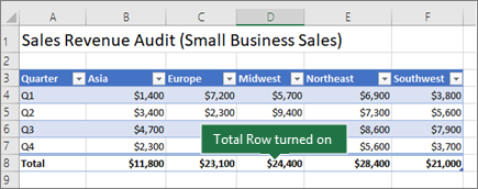
Total the data in an Excel table
You can quickly total data in an Excel table by enabling the Total Row option, and then use one of several functions that are provided in a drop-down list for each table column. The Total Row default selections use the SUBTOTAL function, which allow you to include or ignore hidden table rows, however you can also use other functions.

-
Click anywhere inside the table.
-
Go to Table Tools > Design, and select the check box for Total Row.

-
The Total Row is inserted at the bottom of your table.
Note: If you apply formulas to a total row, then toggle the total row off and on, Excel will remember your formulas. In the previous example we had already applied the SUM function to the total row. When you apply a total row for the first time, the cells will be empty.
-
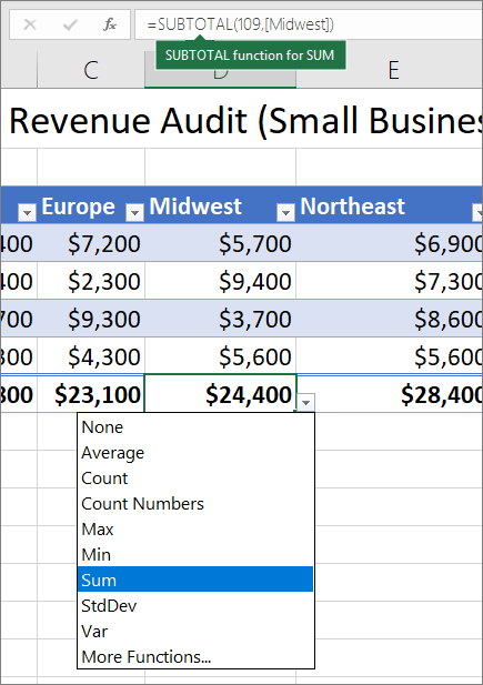
Select the column you want to total, then select an option from the drop-down list. In this case, we applied the SUM function to each column:
You’ll see that Excel created the following formula: =SUBTOTAL(109,[Midwest]). This is a SUBTOTAL function for SUM, and it is also a Structured Reference formula, which is exclusive to Excel tables. Learn more about Using structured references with Excel tables.
You can also apply a different function to the total value, by selecting the More Functions option, or writing your own.
Note: If you want to copy a total row formula to an adjacent cell in the total row, drag the formula across using the fill handle. This will update the column references accordingly and display the correct value. If you copy and paste a formula in the total row, it will not update the column references as you copy across, and will result in inaccurate values.

You can quickly total data in an Excel table by enabling the Total Row option, and then use one of several functions that are provided in a drop-down list for each table column. The Total Row default selections use the SUBTOTAL function, which allow you to include or ignore hidden table rows, however you can also use other functions.
-
Click anywhere inside the table.
-
Go to Table > Total Row.
-
The Total Row is inserted at the bottom of your table.
Note: If you apply formulas to a total row, then toggle the total row off and on, Excel will remember your formulas. In the previous example we had already applied the SUM function to the total row. When you apply a total row for the first time, the cells will be empty.
-
Select the column you want to total, then select an option from the drop-down list. In this case, we applied the SUM function to each column:
You’ll see that Excel created the following formula: =SUBTOTAL(109,[Midwest]). This is a SUBTOTAL function for SUM, and it is also a Structured Reference formula, which is exclusive to Excel tables. Learn more about Using structured references with Excel tables.
You can also apply a different function to the total value, by selecting the More Functions option, or writing your own.
Note: If you want to copy a total row formula to an adjacent cell in the total row, drag the formula across using the fill handle. This will update the column references accordingly and display the correct value. If you copy and paste a formula in the total row, it will not update the column references as you copy across, and will result in inaccurate values.
You can quickly total data in an Excel table by enabling the Toggle Total Row option.
-
Click anywhere inside the table.
-
Click the Table Design tab > Style Options > Total Row.
The Total row is inserted at the bottom of your table.
Set the aggregate function for a Total Row cell
Note: This is one of several beta features, and currently only available to a portion of Office Insiders at this time. We’ll continue to optimize these features over the next several months. When they’re ready, we’ll release them to all Office Insiders, and Microsoft 365 subscribers.
The Totals Row lets you pick which aggregate function to use for each column.
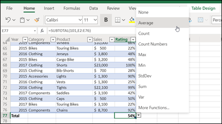
-
Click the cell in the Totals Row under the column you want to adjust, then click the drop-down that appears next to the cell.
-
Select an aggregate function to use for the column. Note that you can click More Functions to see additional options.
Need more help?
You can always ask an expert in the Excel Tech Community or get support in the Answers community.
See Also
Overview of Excel tables
Video: Create an Excel table
Create or delete an Excel table
Format an Excel table
Resize a table by adding or removing rows and columns
Filter data in a range or table
Convert a table to a range
Using structured references with Excel tables
Subtotal and total fields in a PivotTable report
Subtotal and total fields in a PivotTable
Excel table compatibility issues
Export an Excel table to SharePoint
Need more help?
Want more options?
Explore subscription benefits, browse training courses, learn how to secure your device, and more.
Communities help you ask and answer questions, give feedback, and hear from experts with rich knowledge.