
Содержание
- How to See The Current Sheet Number & Total Number of Excel-Sheets
- What the “Sheet Number” feature does
- Availability of the feature in Excel
- How to see the sheet number and the total number of worksheets
- Alternatives
- Total number of sheets (and more) in the “Workbook Statistics”
- Worksheet overview with an Excel Add-In
- Count Sheets in Excel (using VBA)
- Count All Sheets in the Workbook
- VBA Code to Show Sheet Count in a Message Box
- Getting Sheet Count Result in Immediate Window
- Formula to Get Sheet Count in the Worksheet
- Count All Sheets in Another Workbook (Open or Closed)
- Sheet Count in Another Open Workbook
- Sheet Count from a Closed Workbook
- Count All Sheets that Have a Specific Word In It
- Count total values across multiple sheets
- 3 Answers 3
- Function SHEETS and formulas for working with other sheets in Excel
- Formulas using links to other Excel sheets
- SHEETS function to count the number of sheets in a workbook
- Links to other sheets in document templates
How to See The Current Sheet Number & Total Number of Excel-Sheets

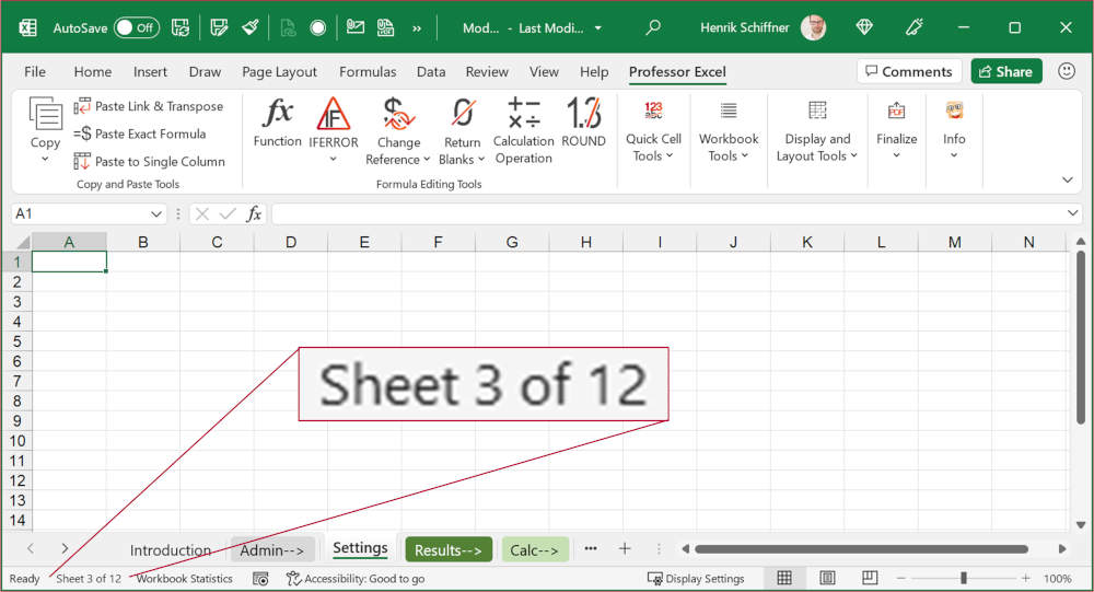
Working with large Excel files with many worksheets can be frustrating. Especially finding things and keeping an overview is troublesome. One (small) feature might come in handy: See the sheet number of the current worksheet and the total number of worksheets. For example, like this: “Sheet 5 / 12”. You can enable this with just a click in the Status Bar.
What the “Sheet Number” feature does
The sheet number feature in Excel does the following:
 Display the current sheet number and total number of worksheets in the bottom-left corner of the Excel window.
- It shows the number of the worksheet that is currently selected in the Status Bar in the left-bottom corner of the Excel window.
- The sheets are counted from left to right. So, if you move a worksheet the numbering changes accordingly (don’t mix it up with the sheet names in the background, for example “Sheet1” etc.).
- It also shows the total number of worksheets in the current Excel file.
- Hidden and very hidden sheets are regarded in the total number count.
- When you select multiple worksheets, still the number of the currently active worksheet is shown.
- When you click on the Sheet Number, the Navigation Pane opens. The current worksheet is then highlighted (with bold font) in the Navigation Pane.
Availability of the feature in Excel
As of now (August 2021), this feature is not available for everyone. Probably, it will sooner or later be rolled out to every user.
- The feature to display the sheet number is first introduced in Excel version 2108 (so the release of August 2021) with Office 365 (now Microsoft 365).
- Initially, the sheet number feature is only available for Office Insider subscribers (for those users who test “beta” versions – not the majority of Excel users). Usually within the next months it’s also available for regular Office 365 subscribers.
- It is at first only available in Office for Windows (not Mac or Office Web / Online).
How to see the sheet number and the total number of worksheets
After knowing now what this feature does and who can use it, it’s time for activating it:
- Right-click on the status bar.
- Set the checkmark at “Sheet number”. Again, if you don’t see such entry please read the section above.
That’s it, now you should see something like “Sheet 3 of 12” in the bottom-left corner of the Excel window.
Alternatives
Total number of sheets (and more) in the “Workbook Statistics”
Excel has another function, called “Workbook Statistics”. It shows very similar information (although not the current worksheet number). It is available already on Windows, Mac and the web version of Excel.
You can activate it by right-clicking on the status bar and then on “Workbook Statistics”.
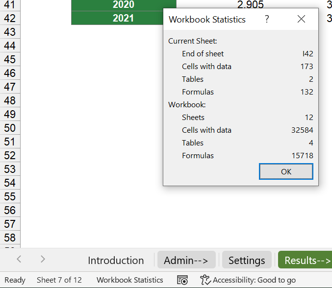 “Workbook Statistics” shows a summary of the Excel file.
Worksheet overview with an Excel Add-In
Because keeping an overview of the workbook is especially for larger Excel files difficult, we have integrated several features into our Excel add-in “Professor Excel Tools”. For example, the “Sheet Manager”, which provides a simple and powerful summary of all your worksheets.
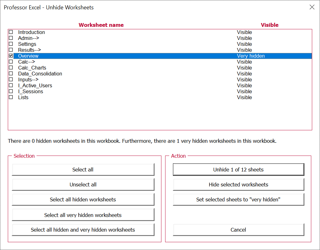 “Professor Excel Tools” has a powerful worksheet manager.

This function is included in our Excel Add-In ‘Professor Excel Tools’
(No sign-up, download starts directly)
More than 35,000 users can’t be wrong.
Источник
Count Sheets in Excel (using VBA)
There are some simple things that are not possible for you to do with in-built functions and functionalities in Excel, but can easily be done using VBA.
Counting the total number of sheets in the active workbook or any other workbook on your system is an example of such a task.
In this tutorial, I’ll show you some simple VBA code that you can use to count the total number of sheets in an Excel workbook.
This Tutorial Covers:
Count All Sheets in the Workbook
There are multiple ways I can use VBA to give me the total count of sheets in a workbook.
In the following sections, I will show you three different methods, and you can choose which one to use:
- Using the VBA code in a module (to get sheet count as a message box)
- Using Immediate window
- Using a Custom Formula (which will give you the sheet count in a cell in the worksheet)
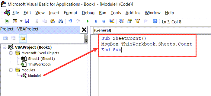
VBA Code to Show Sheet Count in a Message Box
Below is the VBA code to get the total number of sheets in the current workbook shown in a message box:
In the above code, I have used Sheets, which will count all the sheets (be it worksheets or chart sheets). In case you only want to count the total number of worksheets, use Worksheets instead of Sheets. In most cases, people only use worksheets, using Sheets works fine. In layman terms, Sheets = Worksheets + Chart Sheets
Below are the steps to put this code in the VBA Backend:
- Click the Develope tab in the ribbon (don’t see the Developer tab – click here to know how to get it)

- In the Visual Basic Editor that opens, click on ‘Insert’ option in the menu
- Click on Module. This will insert a new module for the workbook

- Copy and Paste the above VBA code in the code window of the module
- Place the cursor anywhere in the code and press the F5 key (or click the green play button in the toolbar)
The above steps would run the code and you will see a message box that shows the total number of worksheets in the workbook.

Note: If you want to keep this code and reuse it in the future in the same workbook, you need to save the Excel file as a macro-enabled file (with a .XLSM extension). You will see this option when you try to save this file.
Getting Sheet Count Result in Immediate Window
The Immediate window gives you the result right there with a single line of code.
Below are the steps to get the count of sheets in the workbook using the immediate window:
- Click the Develope tab in the ribbon (don’t see the Developer tab – click here to know how to get it)
- Click on Visual Basic icon
- In the VB Editor that opens, you might see the Immediate Window already. If you don’t, click the ‘View’ option in the menu and then click on Immediate Window (or use the keyboard shortcut – Control + G)

- Copy and paste the following line of code: ? ThisWorkbook.Sheets.Count

- Place the cursor at the end of the code line and hit enter.
When you hit enter in Step 5, it executes the code and you get the result in the next line in the immediate window itself.
Formula to Get Sheet Count in the Worksheet
If you want to get the sheet count in a cell in any worksheet, using the formula method is the best way.
In this method, I will create a custom formula that will give me the total number of sheets in the workbook.
Below is the code that will do this:
You need to place this code in the module (just like the way I showed in the ” VBA Code to Show Sheet Count in a Message Box” section)
Once you have the code in the module, you can get the sheet count by using the below formula in any cell in the workbook:

Pro Tip: If you need to get the sheet count value often, I would recommend copying and pasting this formula VBA code in the Personal Macro Workbook. When you save a VBA code in the Personal Macro Workbook, it can be used on any Excel file on your system. In short, VBA codes in PMW are always available to you on your system.
Count All Sheets in Another Workbook (Open or Closed)
In the above example, I showed you how to count the number of sheets in the active workbook (the one where you’re working and where you added the VBA codes).
You can also tweak the code a little to get the sheet count in other workbooks (whether open or closed).
Sheet Count in Another Open Workbook
Suppose I want to know the sheet count of an already open workbook – Example.xlsx
The below VBA code with do this:
And in case you want to get the result in the immediate window, you can use the below code.
Sheet Count from a Closed Workbook
In case you need to get the sheet count of a file that’s closed, you either need to open it and then use the above codes, or you can use VBA to first open the file, then count the sheets in it, and then close it.
The first step would be to get the full file location of the Excel file. In this example, my file location is “C:UserssumitOneDriveDesktopTestExample File.xlsx”
You can get the full file path by right-clicking on the file and then clicking on the Copy Path option (or click on the Properties option).
Below are the VBA codes to get the sheet count from the closed workbook:
The above code first opens the workbook, then counts the total number of sheets in it, and then closes the workbook.
Since the code needs to do some additional tasks (apart from counting the sheets), it has some extra lines of code in it.
The Application.DisplayAlerts = False part of the code makes sure that the process of opening a file, counting the sheets, and then closing the file is not visible to the user. This line stops the alerts of the Excel application. And at the end of the code, we set it back to True, so things get back to normal and we see the alerts from thereon.
Count All Sheets that Have a Specific Word In It
One useful scenario of counting sheets would be when you have a lot of sheets in a workbook, and you only want to count the number of sheets that have a specific word in them.
For example, suppose you have a large workbook that has sheets for multiple departments in your company, and you only want to know the sheet count of the sales department sheets.
Below is the VBA code that will only give you the number of sheets that have the word ‘Sales’ in it
Note that the code is case-sensitive, so ‘Sales’ and ‘sales’ would be considered different words.
The above uses an IF condition to check the name of each sheet, and if the name of the sheet contains the specified word (which is checked using the INSTR function), it counts it, else it doesn’t.
So these are some simple VBA codes that you can use to quickly get a count of sheets in any workbook.
I hope you found this tutorial useful!
Other Excel tutorials you may also find useful:
Источник
Count total values across multiple sheets
I have the following data in my Excel file:
Sheet 1
Sheet 2
Sheet 3
I want to get all the records across the multiple sheets and come up with an Excel sheet that summarizes the top products:
Summary
Any way to do this?

3 Answers 3
1) The data in each tab begins in row 2 of columns A to B, with Product in column A
2) In none of these tabs does the data go beyond row 1000 (change all occurrences in the formulas (and Named Ranges) of this value to a suitably larger number if it does)
3) There are no blank cells in between the data in any of your tabs
4) You are using Excel 2007 or later
then, firstly, list all of your relevant sheet names (excluding the Summary sheet) in a horizontal range in your Summary sheet somewhere, e.g. D1:F1, making sure that you list them precisely as they appear on the tabs.
Secondly, go to Name Manager and define two new names:
Refers to: =MMULT(TRANSPOSE(COUNTIFS(INDIRECT(«‘»&$D$1:$F$1&»‘!A2:A1000»),A$2:A2,INDIRECT(«‘»&$D$1:$F$1&»‘!A2:A1000″),»<>«)),ROW(INDIRECT(«1:»&COUNTA(A$2:A2)))^0)
Refers to: =SUBTOTAL(3,INDIRECT(«‘»&$D$1:$F$1&»‘!A2:A1000»))
(Be sure when you create these that they appear exactly as here. Sometimes, if pasted in, you can end up with quotation marks around the formulas, which is not correct.)
In cell A2 of the Summary sheet enter:
(Or whatever the name of your first sheet is.)
Then, in A3 of the Summary sheet, this array formula**:
Copy down until you start to get blanks.
Again, copy down until you start to get blanks.
**Array formulas are not entered in the same way as ‘standard’ formulas. Instead of pressing just ENTER, you first hold down CTRL and SHIFT, and only then press ENTER. If you’ve done it correctly, you’ll notice Excel puts curly brackets <> around the formula (though do not attempt to manually insert these yourself).
Источник
Function SHEETS and formulas for working with other sheets in Excel
SHEET function is designed to return the number of a specific sheet with a space, which allows access to the entire workbook in MS Excel. SHEETS function provides the user with information on the number of sheets contained in the workbook.
Formulas using links to other Excel sheets
Suppose we have a company DecArt in which employees work and their monthly, salary is calculated. This company has information about the average monthly salary in Excel, and the data on it are placed on different sheets: on sheet 1 there are data on wages, on sheet 2, the percentage bonus. We need to calculate the size of the premium in dollars, while these data were placed on the second sheet.
To begin, consider an example of working with sheets in Excel formulas. Example 1:
- Let’s create on sheet 1 of the workbook of the spreadsheet Excel processor table, as shown in the figure. Information about the average monthly wage:

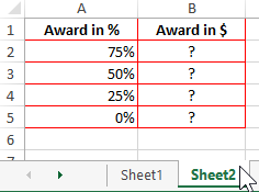
- Next, on sheet 2 of the workbook, we will prepare an area for placing our result — the size of our premium in dollars, as shown in the figure:
- Next, we will need to enter into the B2 cell the formula shown in the figure below:
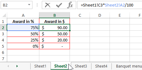
This formula was entered as follows: first, in cell B2, we set the «=» sign, then clicked on «Sheet1» in the lower left corner of the workbook and went to cell C3 on sheet 1, then entered the multiplication operation and switched again to «Sheet2 «to add a percentage.
Thus, when calculating the bonus of each employee, we obtained the initial data on one sheet, and the calculation was made on another sheet. This formula will be very useful when working with longer data sets in large organizations.
SHEETS function to count the number of sheets in a workbook
Consider now the example of the function. It often happens that there are too many sheets in an Excel workbook. It is not possible to visually find out their exact number; it is for this purpose that the SHEETS function has been created.
In this function, only 1 argument — «Link» and even then optional. If it is not filled, then the function returns the total number of sheets created in the current workbook of the Excel file. If necessary, you can fill in the argument. To do this, it is necessary to specify a link to the workbook, in which you need to calculate the total number of sheets created in it.
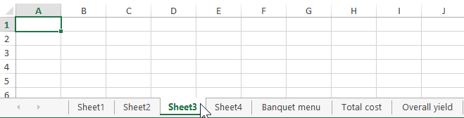
Example 2. Suppose we have a firm for the production of upholstered furniture, and it has a lot of documents that are contained in the Excel workbook. We need to calculate the exact number of these documents, since each of them has its own name, then it will take time to visually calculate their number.
The figure below shows the approximate number:
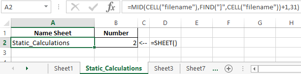
To organize the counting of all sheets, you must use function. Simply set the equal sign “=” and enter the function without filling its arguments in brackets. The call to this function is shown below:
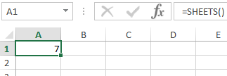
As a result, we obtain the following value: 12 sheets.
Thus, we learned that our company has 12 documents contained in an Excel workbook. This simple example clearly illustrates the operation of the function. This feature can be useful for managers, office workers, sales managers.
Links to other sheets in document templates
Example 3. There are data on the cost of a banquet company engaged in on-site service. It is necessary to calculate the total cost of the banquet, as well as the total yield of portions of dishes, and calculate the total number of sheets in the document.
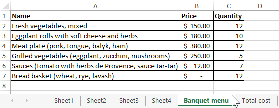
- Create a table «Banquet menu», a general view of which is shown in the figure below:
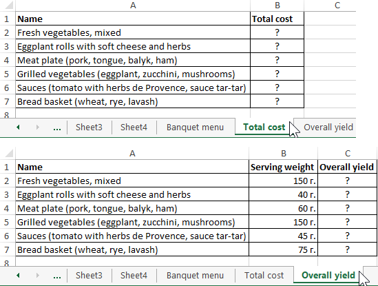
- Similarly, create tables on different sheets «Total cost» and «Total output»:
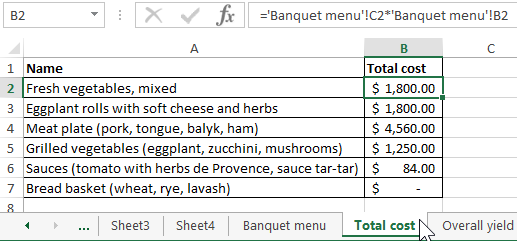
- Using the formula with links to other sheets, we will calculate the total cost of the banquet menu:
- Let’s go to the sheet “Total yield” and by multiplying the cells of the weight of one portion, located on sheet 2 and the total number, located on sheet 1, we will calculate the total output:
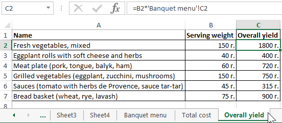
As a result, we got the simplest template for calculating the cost of 1 banquet.
Источник
If you’ve ever had to sum up items across many different sheets, then you know it can be a real pain when there are a lot of sheets. This trick will make it super easy.
Get the example workbook with the above link to follow along.
In this example, you have a table of sales figures each in a separate tab named Jan through Dec.
Each sheet is the same format with the table in the same position within each sheet.
=Jan!C3+Feb!C3+Mar!C3+Apr!C3+May!C3+Jun!C3+Jul!C3+Aug!C3+Sep!C3+Oct!C3+Nov!C3+Dec!C3If you wanted to create a Total sheet and have a table in it that sums up each of the tables in the Jan to Dec sheets, then you could use the above formula and copy it across the whole table.
Creating this formula isn’t very efficient though, as it requires selecting the Jan sheet, then selecting the cell C3, then typing a +, then selecting the Feb sheet, etc.s
Going through 12 sheets in all. There is a better way!
Add the sum formula into the total table.
- Type out the start of your sum formula
=SUM(. - Left click on the Jan sheet with the mouse.
- Hold Shift key and left click on the Dec sheet. Now select the cell C3 in the Dec sheet. Add a closing bracket to the formula and press Enter.
Your sum formula should now look like this =SUM(Jan:Dec!C3).
The formula will sum up C3 across each of the sheets from Jan to Dec.
You can also use this technique with other formulas like COUNT, AVERAGE, etc. An easier way over cycling through each sheet individually.
About the Author
John is a Microsoft MVP and qualified actuary with over 15 years of experience. He has worked in a variety of industries, including insurance, ad tech, and most recently Power Platform consulting. He is a keen problem solver and has a passion for using technology to make businesses more efficient.
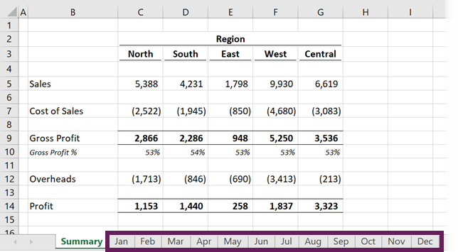
Have you ever had to sum the same cell across multiple sheets? This often occurs where information is held in numerous sheets in a consistent format. For example, it could be a monthly report with a tab for each month (see screenshot below as an example).
Watch the video
Watch the video on YouTube.
I see many examples where the user has clicked the same cell on each sheet, putting a “+” symbol between each reference. If there are a lot of worksheets, it takes a while to click on them all. Also, if the sheet names are long, the formula starts to look quite unreadable. The screenshot below shows an example of this type of approach.
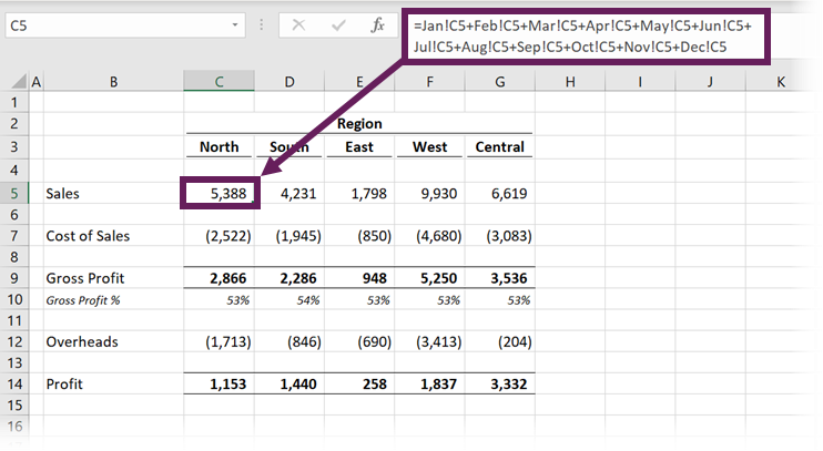
The formula in cell C5 is:
=Jan!C5+Feb!C5+Mar!C5+Apr!C5+May!C5+Jun!C5+
Jul!C5+Aug!C5+Sep!C5+Oct!C5+Nov!C5+Dec!C5
How do you know if you’ve clicked on every worksheet? What if you happened to miss one by accident? There is only one way to know – you’ve got to check it!
The chances are that you don’t need to do all that clicking. And just think about the time you will waste if there is a new tab to be added.
The good news is that there is another approach we can take that will enable us to sum across different sheets easily. I still remember the first time a work colleague showed me this trick; my jaw hit the ground in amazement. I thought he was an Excel genius. That’s why I’m sharing it here; by using this approach, you can look like an Excel genius to your work colleagues too 🙂
To sum the same cell across multiple sheets of a workbook, we can use the following formula structure:
=SUM('FirstSheet:LastSheet'!A1)
- Replace FirstSheet and LastSheet with the worksheet names you wish to sum between. If your worksheet names contain spaces, or are the name of a range (e.g., Q1 could be the name of a sheet or a cell reference ), then single quotes ( ‘ ) are required around the sheet names. If not, the single quotes can be left out.
- Replace A1 with the cell reference you wish to use
With this beautiful little formula, we can see all the worksheets included in the calculation just by looking at the tabs at the bottom. Take a look at the screenshot below. All the tabs from Jan to Dec are included in the calculation.
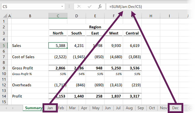
The formula in cell C5 is:
=SUM(Jan:Dec!C5)
SUM across multiple sheets – dynamic
We can change this to be more dynamic, making it even easier to use. Instead of using the names of the first and last tabs, we can create two blank sheets to act as bookends for our calculation.
Take a look at the screenshot below. The Start and End sheets are blank. By dragging sheets in and out of the Start and End bookends, we can sum almost anything we want.
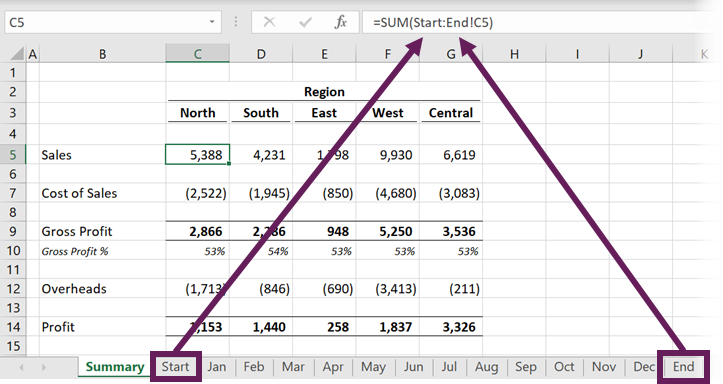
The formula in cell C5 is
=SUM(Start:End!C5)
We can also create sub-calculations. For example, we could add quarters as interim bookends too. There is the added advantage that the tabs also serve as helpful presentation dividers. The example below shows the calculation of just Jan, Feb, and Mar sheets.
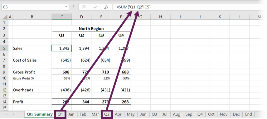
The formula in cell C5 is:
=SUM('Q1:Q2'!C5)
Excel could mistake Q1 and Q2 as cell references; therefore, adding single quotes around the sheet names is essential.
Which other formulas does this work for?
This approach doesn’t just work for the SUM function. Here is a list of all the functions for which this trick works.
| Basic Calculations
SUM AVERAGE AVERAGEA PRODUCT |
Counting
COUNT COUNTA |
Min & Max
MAX MAXA MIN MINA |
Standard deviation
STDEV STDEVA STDEVP STDEVPA |
Variance
VAR VARA VARP VARPA |
The drawbacks
There are a few things to be aware of:
- All the sheets must be in a consistent layout and must stay that way. If one worksheet changes, the formula many not sum the correct cells.
- Usually, formula cell references move automatically when new rows or columns are inserted. This formula does not work like that. It will only move if you select all the sheets and then insert a row or column into all of those sheets at the same time.
- Any sheets which are between the two tabs are included within the calculation. Therefore, even though we cannot see them, hidden sheets are also included in the result.

About the author
Hey, I’m Mark, and I run Excel Off The Grid.
My parents tell me that at the age of 7 I declared I was going to become a qualified accountant. I was either psychic or had no imagination, as that is exactly what happened. However, it wasn’t until I was 35 that my journey really began.
In 2015, I started a new job, for which I was regularly working after 10pm. As a result, I rarely saw my children during the week. So, I started searching for the secrets to automating Excel. I discovered that by building a small number of simple tools, I could combine them together in different ways to automate nearly all my regular tasks. This meant I could work less hours (and I got pay raises!). Today, I teach these techniques to other professionals in our training program so they too can spend less time at work (and more time with their children and doing the things they love).
Do you need help adapting this post to your needs?
I’m guessing the examples in this post don’t exactly match your situation. We all use Excel differently, so it’s impossible to write a post that will meet everybody’s needs. By taking the time to understand the techniques and principles in this post (and elsewhere on this site), you should be able to adapt it to your needs.
But, if you’re still struggling you should:
- Read other blogs, or watch YouTube videos on the same topic. You will benefit much more by discovering your own solutions.
- Ask the ‘Excel Ninja’ in your office. It’s amazing what things other people know.
- Ask a question in a forum like Mr Excel, or the Microsoft Answers Community. Remember, the people on these forums are generally giving their time for free. So take care to craft your question, make sure it’s clear and concise. List all the things you’ve tried, and provide screenshots, code segments and example workbooks.
- Use Excel Rescue, who are my consultancy partner. They help by providing solutions to smaller Excel problems.
What next?
Don’t go yet, there is plenty more to learn on Excel Off The Grid. Check out the latest posts:
See all How-To Articles
This tutorial demonstrates how to count the number of worksheets in an Excel file.
Count Number of Worksheets
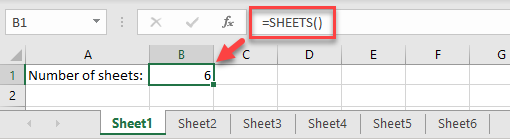
The easiest way to count the number of worksheets in your workbook is to use the SHEETS Function. Say your Excel file has six worksheets.
In any cell on any of the sheets, enter the formula:
=SHEETS()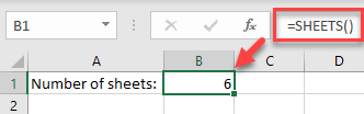
As you can see, this function without arguments returns the total number of sheets in the current workbook (including hidden sheets).
In this article, we will learn how to get the sum or add cells across multiple sheets in Microsoft Excel.
Sometimes we need to access different values from different worksheets of the same excel book. Here we are accessing it to add multiple cells in Excel 2016.
In this article, we will learn how to sum the values located on different sheets in excel 2016. We will use the SUM function to add numbers.
SUM function adds up the values.
SUM = number 1 + number 2 + …
Syntax:
=SUM(number 1, number 2, ..)
Let’s understand how to add cells in excel 2016 with the example explained here.
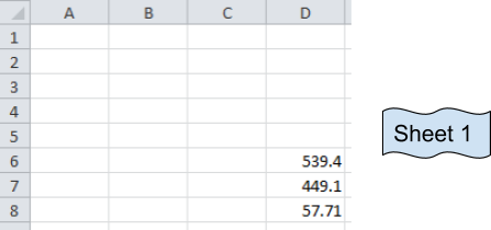
These are numbers from three different sheets and desired output sum will be in Sheet 1.
Now we use the SUM function
Formula:
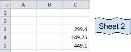
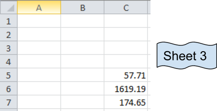
=SUM(D6:D8, Sheet2!C3:C5,Sheet3!C5:C7)
Explanation:
The resulting output is in Sheet 1.
D6:D8 adds the values of Sheet 1 D6+D7+D8
C3:C5 adds the values of Sheet 2 C3+C4+C5
C5:C7 adds the values of Sheet 3 C5+C6+C7.
It’s basically the addition of values in cells
D6+D7+D8 + C3+C4+C5 + C5+C6+C7
You can select the cells separated by commas to add the numbers.
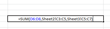
Your formula will look like the above image.
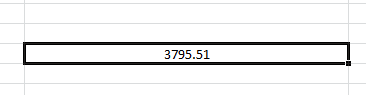
Press Enter and your desired sum will be here in Sheet 1.
As we can see Sum function returns the sum. You can use Autosum option in Home tab in Editing.
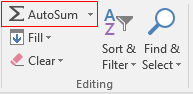
Click arrow key for more options like shown below.
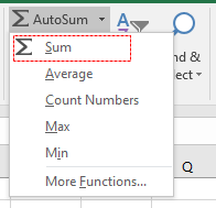
Then select the cells to add up values in Excel. You can sum across the rows and columns using the SUM function.
Hope you got SUM function adding cells in excel. The same function can be performed in Excel 2016, 2013 and 2010. Let us know how you like this article. You will find more content on functions and formulas here. Please state your query down in the comment box. We will help you.
If you liked our blogs, share it with your friends on Facebook. And also you can follow us on Twitter and Facebook. Hope you got SUM function adding cells in excel. The same function can be performed in Excel 2016, 2013 and 2010. Let us know how you like this article. You will find more content on functions and formulas here. Please state your query down in the comment box. We will help you.
We would love to hear from you, do let us know how we can improve, complement or innovate our work and make it better for you. Write us at info@exceltip.com
Popular Articles:
50 Excel Shortcut to Increase Your Productivity
How to use the VLOOKUP Function in Excel
How to use the COUNTIF function in Excel
How to use the SUMIF Function in Excel