
Содержание
- Quick Access Toolbar in Excel
- Practical use of the Quick Access Toolbar
- Customize the Excel shortcut bar
- The advanced Setup
- Changing of the location
- Excel Toolbar
- Introduction to Toolbar in Excel
- How to Use the Toolbar in Excel?
- Example #1
- Example #2
- Example #3
- Example #4
- Example #5
- Things to Remember
- Recommended Articles
- Toolbar on Excel
- Excel Toolbar
- How to Use the toolbar in Excel?
- Examples to Understand Quick Access Excel Toolbar
- 1 – Adding Features to the Toolbar
- #2 – Deleting Features from the Toolbar
- #3 – Moving the Toolbar on the Ribbon
- #4 – Modifying the Sequence of Commands and Resetting to Default Settings.
- #5 – Customize Excel Toolbar
- #6 – Exporting and Importing of Quick Access Toolbar
- Things to Remember
- Recommended Articles
The name of the Quick Access Toolbar speaks for itself. Here are placed those tools, that the user uses most often. Moreover, here you can place tools that are not in the strip with bookmarks. For example, the «PivotTable Wizard», etc.
The Quick Access Toolbar – is the first best solution for users, who are migrating from older versions of Excel and do not have time to the learning of the new interface or its settings, but want to start working right away.
This panel is still useful in the mode of the folded main band of tools. Then there is not necessary to leave the convenient for viewing and working mode with folded strip each time.
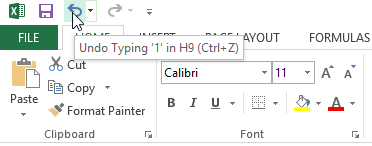
There is the Excel shortcut bar above of the wide tool bar. By default, there are 3 most frequently used tools:
- Save (CTRL + S).
- Cancel the input (CTRL + Z).
- Repeat input (CTRL + Y).
The amount of tools in the Quick Access Toolbar can be changed with using the setting.
- When downloading the program, the active cell on the blank sheet is located at A1 address. Type the letter «a» from the keyboard and press «Enter». The cursor will move down to the cell A2.
- Click the «Undo Input» tool (or the hotkey combination: CTRL + Z) and the text disappears, but the cursor returns to the starting position.

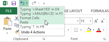
- If you perform to several actions on the worksheet (for example, fill in several letters with the letters), then the drop-down list of the action history for the «Cancel input» button will be available for you. Thus, you can cancel a lot of actions with one click, which is very convenient.
After of the canceling several actions, the history list for the «Repeat Input» tool is available.
Customize the Excel shortcut bar
The Quick Access Toolbar – is the flexible toolbar in Excel for simplifying and improving the user experience in the program.
You can place buttons of frequently used tools. Try adding the «Create» tool button yourself.
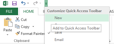
- On the right side, click on the drop-down list to call up the configuration options.
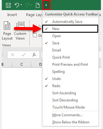
- From the list that appears, select the «New» option and add the tool for creating new Excel workbooks.
- Mark again the option «Create» from the list of settings to delete this tool.
The advanced Setup
In the panel setup options, using the drop-down list, only a few popular tools, but you can add to the panel any of tool available in Excel.
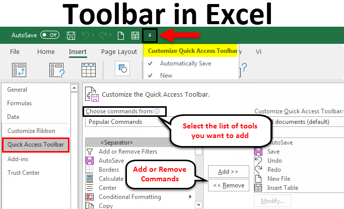
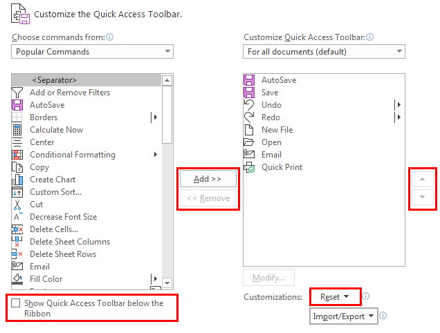
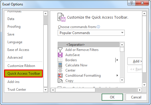
- To flexibly configure the contents of the Quick Access Toolbar, you must select the «Other Commands» option. The «Excel Options» window appears with the parameter «Quick Access Toolbar» already selected. To call this window you can and through the «File» option «Options», then select the necessary option.
- Select the tool in the left list, that you want to use often. Click on the «Add» button and press OK.
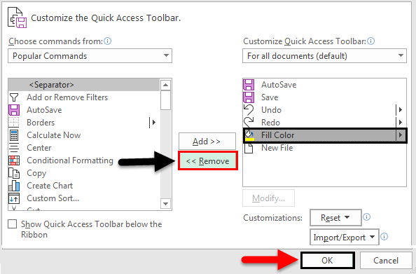
- To remove tools, select the tool from the right list and click on the «Delete» button, then OK.
Changing of the location
If necessary, this panel can be placed under the tool bar, not above it.
Open the drop-down list and select the «Place below the ribbon» option. This task can also be solved by using the context menu. To open the context menu, you need to right-click on the panel.
To return the panel back (by placing it over the tape), select the «Place over tape» option in the same way.
Источник
Excel Toolbar (Table of Contents)
The Toolbar is an area where you can add different commands or tools associated with excel. By default, it is located above the ribbon with different tools and visible in the Excel window’s upper right corner. To increase customer friendliness, toolbars have become customizable according to the frequent use of different tools. Instead of a set of tools, excel gives us the option to select and build a Quick Access Toolbar. This makes quick access to the tools that you want. So the toolbar is popularly known as Quick Access Toolbar.
Excel functions, formula, charts, formatting creating excel dashboard & others

It is a symbolical representation of built-in options available in Excel. By default, it contains the below commands.
- Save: To save the created workbook.
- Undo: To return or step back one level of an immediate action performed.
- Redo: Repeat the last action.
How to Use the Toolbar in Excel?
The Toolbar in Excel is a shortcut tool to avoid searching for the commands you often use in the worksheet. Using Toolbar in Excel is easy, and it helps us simplify access to the document’s commands. Let’s understand the working of the Toolbar in Excel by some examples given below.
Example #1
Adding Commands to the Toolbar in Excel
To get more tools, you have the option to customize the Quick Access Toolbar simply by adding the commands.
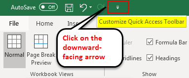
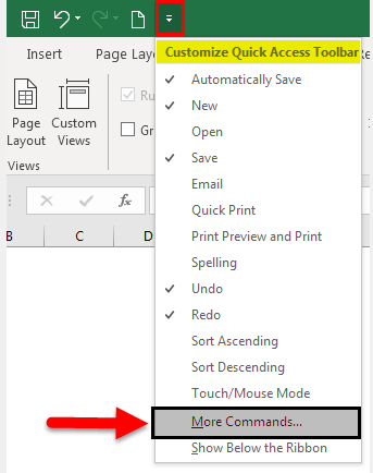
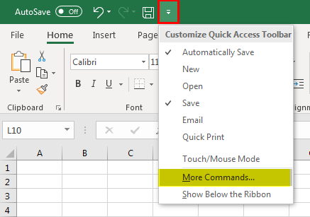
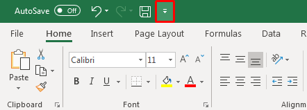
- Click on the downward-facing arrow at the end of the Toolbar in Excel. A pop up will be shown as Customize Quick Access Toolbar.
- From the dropdown, you will get a list of commonly used commands. Click any of the options that you want, and it will be added to the toolbar.
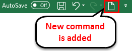
- A new command is selected, and this will be added to the toolbar highlighted as the command is added with already available tools.
In a similar way, you can add the tools which you want to access quickly. So instead of clicking and finding the tools from the multiple hierarchies, you can access the option within a single click.
Example #2
Adding Commands to the Toolbar in Excel
There are options to add more tools Instead of the listed commands. You can add more commands to the quick Access Toolbar by selecting More Commands.
- Click on the downward-facing arrow at the end of the toolbar. Select the More Commands option.
- You will get a new window which gives you all the options available with excel to add to your toolbar.
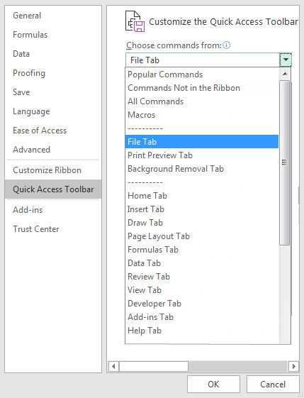
From the Choose commands from the drop-down, you can select which list of tools you want to add. Each list will lead to a different list of commands that you can add to the toolbar.
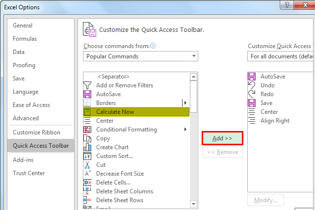
- Click on the Popular Commands, which shows the set of most commonly used commands. Select the Fill color which you want to add to the toolbar. You can see an add button right next to the list of commands; by pressing it and clicking on the OK button, you can add the selected tool to the Excel Toolbar.
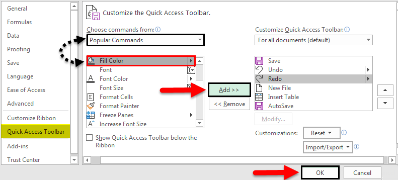
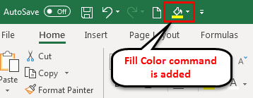
- Once you add the command, it will appear in the list next to the add button. This is the list of tools added to the Toolbar. The “Fill Color” command will be added to the Customize Quick Access Toolbar.
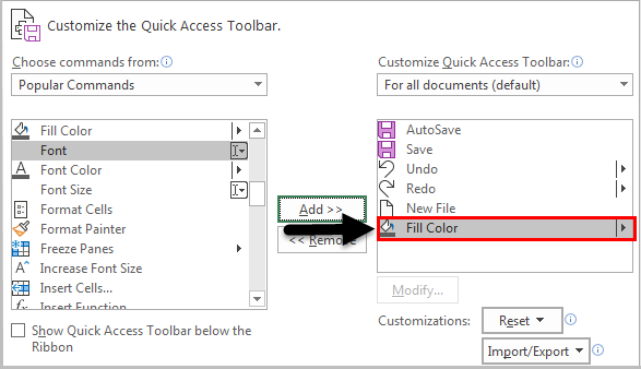
- You can see the “Fill Color” command added to the Quick Access Toolbar as below and the existing commands. Since this is the last item added to the Quick Access Toolbar, it will appear in the listed order.
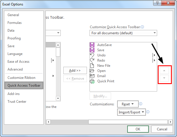
- To reorder the added items, you can use the up and down arrow highlighted on the right to the list of items.
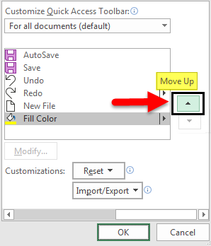
- Select the command which you want to reorder or change the position. By clicking the Upward arrow, the “Fill Color” command is moved upwards in the list shown as below.
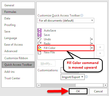
- By pressing the OK button, the selected format will be applied to the Quick Access Toolbar. The “Fill Color” Command is visible before the “New File” Tool.
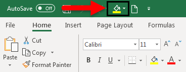
You can see the visibility order of the listed tools is changed. According to the new list order, the “Fill Color” position has been changed to the second last from the end.
Example #3
Removing Command
The commands can be removed from the quick access toolbar if you are no longer using them or not using them frequently. The commands can be removed in a similar way to how you added the commands to the Quick Access Toolbar.
- Click on the downward-facing arrow at the end of the toolbar. Select the More Commands option.
- You will get a new window which will show the already added commands on the right side. This is the list of commands which are already in the quick access toolbar.
- Select the command which you want to remove from the quick access toolbar. In the center, below the add button, a Remove button will be enabled. Press the OK button to make the applied changes.
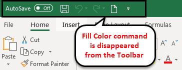
- The Fill Color command is removed, and it will be disappeared from the Quick Access Toolbar, as shown below.
Example #4
Moving the Position
According to your convenience, you can change the position of the toolbar. You can change the position from top to below the ribbon or vice versa.
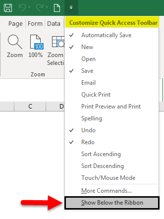
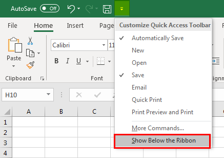
- Select the downward-facing arrow at the end of the toolbar, then select the Show Below the Ribbon option from the list.
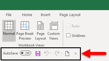
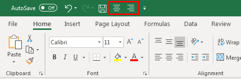
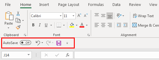
- Now the Toolbar is moved below to the ribbon.
Example #5
Adding Ribbon Commands
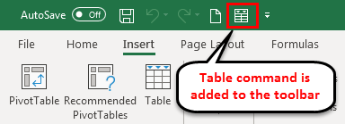
- Right-click on the tool within the ribbon which you want to add to the Toolbar in Excel. You will get the option to Add to Quick Access Toolbar. Here we right-clicked on the Table tool to add from the insert command.
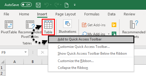
- The command will be added to the Quick Access Toolbar as below.
Things to Remember
- Similar to the name Quick Access Toolbar, this is a customizable toolbar to access the tools easily.
- It is possible to add any of the available commands in excel to the Excel Toolbar.
- The visibility of the toolbar can be set above or below the ribbon.
- Just through a right-click, you will get the option to add most of the command to the Toolbar in Excel.
Recommended Articles
This has been a guide to Toolbar in excel. Here we have discussed How to Use and Customize the Toolbar in Excel, along with practical examples. You can also go through our other suggested articles –
Источник


Toolbar or we can say it is a Quick Access Toolbar available in Excel on the left top side of the Excel window. By default, it has only a few options such as “Save,” “Redo,” and “Undo,” but we can customize the toolbar as per our choice and insert any option or button in the toolbar which will help us to reach the commands to use more quickly than before.
Table of contents
Excel toolbar (also called Quick Access Toolbar Quick Access Toolbar Quick Access Toolbar (QAT) is a toolbar in Excel that may be customized and is located on the upper left-hand side of the window. It enables users to save important shortcuts and easily access them when needed. read more ) is presented to access various commands to perform the operations. In addition, it is presented with an option to add or delete commands to it to access them quickly.
- Quick Access Toolbar is universal, and access is possible on any tab like “Home,” “Insert,” “Review,” “References,” etc. It is independent of the tab that we are working on simultaneously.
- It contains the various options used frequently to enhance the speed of working in Excel sheets.
- Along with the Quick Access Toolbar, another toolbar such as the “Formula Bar,” “Headings,” and Gridlines in excelGridlines In ExcelGridlines are little lines made of dots to divide cells from each other in a worksheet. The gridlines have slight faint invisibility; you can find it in the page layout tab. This option has a checkbox; for activating the gridlines, you can tick on it and untick if you wish to deactivate gridlines.read more under the “Show” or “Hide” group of the “View” tab simply selecting and deselecting the checkmark shows or hides this toolbar.
- “Format” toolbar, “Drawing” toolbar, “Chart” toolbar, and “Standard” toolbar presented in the earlier version of Excel 2003 are modified into the “Home” tab and “Insert” tab in the later versions of Excel 2007 and more.
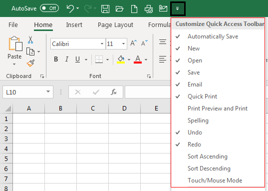
- The “Customize Quick Access Toolbar” option is available to access the full toolbars list.
You are free to use this image on your website, templates, etc., Please provide us with an attribution link How to Provide Attribution? Article Link to be Hyperlinked
For eg:
Source: Toolbar on Excel (wallstreetmojo.com)
How to Use the toolbar in Excel?
- The toolbar in Excel is used for various purposes. However, few major activities are performed on the Quick Access Toolbar on different versions of Excel.
- In the 2007 version, only three activities shift the toolbar’s location, including adding extra features or frequently used commands. In addition, deleting an element from the toolbar is possible whenever we do not want to.
- In higher versions than in 2007, the Quick Access Toolbar is used in many ways, along with adding and removing commands. These include adding commands not presented on the toolbar, modifying commands order, moving the toolbar below or above the ribbon, grouping two or more commands, exporting and importing the toolbar, customizing utilizing the “Options” command, and resetting the default settings.
- Frequent commands like “Save,” “Open,” “Redo,” “New,” “Undo,” “Email,” “Quick Print,” and print preview in excelPrint Preview In ExcelPrint preview in Excel is a tool used to represent the print output of the current page in the excel to see if any adjustments need to be made in the final production. Print preview only displays the document on the screen, and it does not print.read more are easily added to the toolbar.
- We can select the commands not listed in the toolbar from the three categories, including “Popular Commands,” “All Commands,” and “Commands Not Listed” on the ribbon.
Examples to Understand Quick Access Excel Toolbar
Below are examples of the Excel toolbar.
1 – Adding Features to the Toolbar
Adding features or commands to the Quick Access Toolbar is essential. It is done in three ways:
- Adding commands located on the ribbon
- Adding features through the “More Commands” option
- Adding the elements presented on the different tabs directly to the toolbar
Method 1
In the above figure, we can see the tick-marked option present in the toolbar.
Method 2
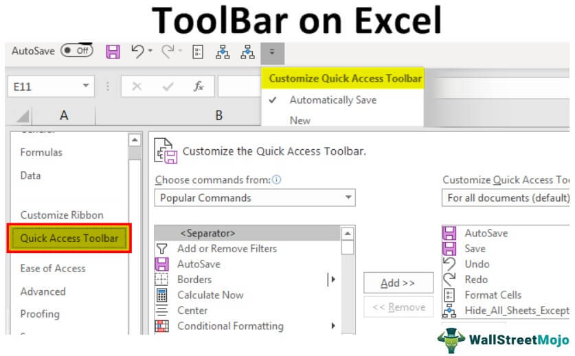
In this, a user must select the “Customize Quick Access Toolbar” in Excel and select the “More Commands” option to add the commands.
As shown in the below figure of the customize window, the user must select the commands and click on the “Add” option to add the feature to the toolbar. Added features are displayed on the excel ribbon Excel Ribbon The ribbon is an element of the UI (User Interface) which is seen as a strip that consists of buttons or tabs; it is available at the top of the excel sheet. This option was first introduced in the Microsoft Excel 2007. read more for accessing easily.
Method 3
The user has to right-click on the feature presented on the ribbon and choose “Add to Quick Access Toolbar.”

As shown in the figure, center and right alignment commands are added to the toolbar utilizing this option.
#2 – Deleting Features from the Toolbar
To remove commands,
Select the command that wants to be removed under the “Customize Quick Access Toolbar” option.
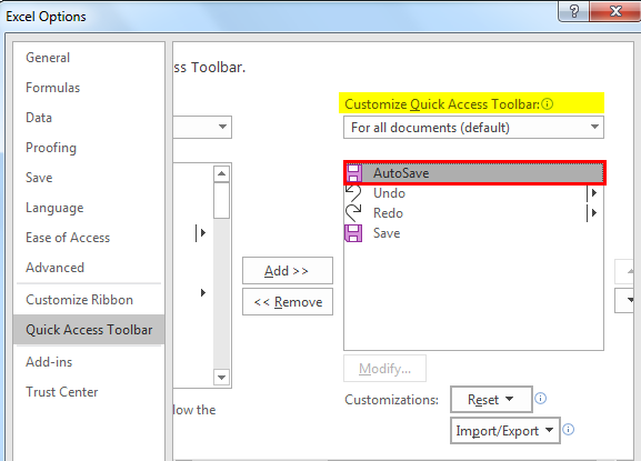
Then, click on the “Remove” button to remove the selected command.

We can also do it by selecting “Excel Options” by clicking on the Microsoft office button on the top left corner of the window and then going to the “Customize” tab.
#3 – Moving the Toolbar on the Ribbon
If a user wants to shift the toolbar to another location, it is done in a few steps. First, the toolbar can be presented below or above the ribbon.
To present the toolbar below the ribbon:
- Click on the “Customize Quick Access Toolbar” button.
- Select the options shown below the ribbon.
#4 – Modifying the Sequence of Commands and Resetting to Default Settings.
The up and down buttons on the “Customize Quick Access Toolbar” present the option in the order per user. Users can discard the changes by clicking on the “Reset” option to get the default settings.
#5 – Customize Excel Toolbar
Customizing the Excel toolbar is done to add, remove, reset, change the toolbar’s location, modify, and alter the order of the features at a time.
All operations are performed quickly on the toolbar using the customization option.
#6 – Exporting and Importing of Quick Access Toolbar
Exporting and importing features are presented in the latest versions of Excel to have the same settings for files used by another computer. To do this,
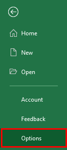
- Go to “File” and select “Options.”
- Then go to a “Quick Access Toolbar.”
- Choose the “Import/Export” option to export customized settings.
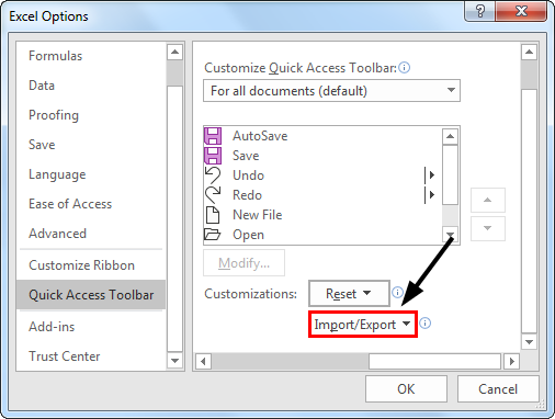
Use the same steps to import customization.
Things to Remember
- The Quick Access Toolbar does not have a feature of displaying multiple lines.
- It is hard to enhance the size of the buttons to correspond to the commands. It is done only by changing the resolution of the screen.
- Another way to add commands to the toolbar is that right-clicking on the ribbon facilitates the option.
- Contents of several commands such as styles, indent, and spacing are not added to the toolbar but are represented in the form of buttons.
- Keyboard shortcutsKeyboard ShortcutsAn Excel shortcut is a technique of performing a manual task in a quicker way.read more are also applied to the commands presented on the toolbar. For example, pressing the “ALT” key displays the shortcut numbers to utilize the commands more effectively by reducing the time.
Recommended Articles
This article is a guide to Toolbar on Excel. Here, we discuss how to add, delete, and modify features on the toolbar and how to customize the Excel toolbar. You can learn more about Excel from the following articles: –
Источник
The name of the Quick Access Toolbar speaks for itself. Here are placed those tools, that the user uses most often. Moreover, here you can place tools that are not in the strip with bookmarks. For example, the «PivotTable Wizard», etc.
The Quick Access Toolbar – is the first best solution for users, who are migrating from older versions of Excel and do not have time to the learning of the new interface or its settings, but want to start working right away.
This panel is still useful in the mode of the folded main band of tools. Then there is not necessary to leave the convenient for viewing and working mode with folded strip each time.
Practical use of the Quick Access Toolbar
There is the Excel shortcut bar above of the wide tool bar. By default, there are 3 most frequently used tools:
- Save (CTRL + S).
- Cancel the input (CTRL + Z).
- Repeat input (CTRL + Y).
The amount of tools in the Quick Access Toolbar can be changed with using the setting.
- When downloading the program, the active cell on the blank sheet is located at A1 address. Type the letter «a» from the keyboard and press «Enter». The cursor will move down to the cell A2.
- Click the «Undo Input» tool (or the hotkey combination: CTRL + Z) and the text disappears, but the cursor returns to the starting position.
- If you perform to several actions on the worksheet (for example, fill in several letters with the letters), then the drop-down list of the action history for the «Cancel input» button will be available for you. Thus, you can cancel a lot of actions with one click, which is very convenient.
After of the canceling several actions, the history list for the «Repeat Input» tool is available.
Customize the Excel shortcut bar
The Quick Access Toolbar – is the flexible toolbar in Excel for simplifying and improving the user experience in the program.
You can place buttons of frequently used tools. Try adding the «Create» tool button yourself.
- On the right side, click on the drop-down list to call up the configuration options.
- From the list that appears, select the «New» option and add the tool for creating new Excel workbooks.
- Mark again the option «Create» from the list of settings to delete this tool.
The advanced Setup
In the panel setup options, using the drop-down list, only a few popular tools, but you can add to the panel any of tool available in Excel.
- To flexibly configure the contents of the Quick Access Toolbar, you must select the «Other Commands» option. The «Excel Options» window appears with the parameter «Quick Access Toolbar» already selected. To call this window you can and through the «File» option «Options», then select the necessary option.
- Select the tool in the left list, that you want to use often. Click on the «Add» button and press OK.
- To remove tools, select the tool from the right list and click on the «Delete» button, then OK.
Changing of the location
If necessary, this panel can be placed under the tool bar, not above it.
Open the drop-down list and select the «Place below the ribbon» option. This task can also be solved by using the context menu. To open the context menu, you need to right-click on the panel.
To return the panel back (by placing it over the tape), select the «Place over tape» option in the same way.
Excel Quick Analysis Tool allows you to quickly analyze data.
It gives you quick access to some of the commonly used data analysis functionalities in Excel so that you don’t have to go into the ribbon and find the correct option (hence saving some clicks and a little bit of time).
In this tutorial, I will tell you everything you need to know about the Quick Analysis Tool in Excel. I’d also cover different use cases where you can use this tool to be more productive and save time.
Where is the Quick Analysis Tool in Excel?
Excel Quick Analysis tool was introduced in Excel 2013, so you won’t find it in versions before Excel 2013.
If you’re searching for the Quick Analysis Tool in the ribbon in Excel, you won’t find it.
It appears automatically whenever you select a range of cells an icon in the bottom right part of the selection.

You can also use the keyboard shortcut Control + Q to show the Quick Analysis Tool icon, in case it doesn’t show up.
By default, this tool is enabled in all the Excel versions (in and after Excel 2013). In case you still can’t access the Quick Analysis Tool, you can follow the steps here to enable it.
What Can You Do with Quick Analysis Tool in Excel?
Quick Analysis Tool tries to give you some commonly used functionalities in Excel.
Note that the data analysis options you see in the Quick Analysis Tool are not unique and you can also find these in the ribbon in different tabs in Excel. The point of showing this tool is to enable you to access these faster.
Let’s now look at all the options you have available in the Quick Analysis Toolbar:
Conditional Formatting
The first option you get in the Quick Analysis Toolbar is Conditional Formatting. Within this, you will see five commonly used Conditional Formatting options.

Note that these options would change based on the data you have selected. For example, if you have numeric data, you will see options such as Data Bars, Icon set, Greater than, Top 10%, etc.
If you have text data, then the options would be to highlight duplicate or unique values or highlight cells that contain specific text or matches a specific string.
And similarly, in case you have dates data, the options would accordingly change.
Keyboard Shortcut - Control + Q + F
Charts
Based on the data in your selected range, you will be shown some commonly used chart types in Excel.

In case you don’t find the chart type you’re looking for, you can click on the More Charts option, which will open the ‘Insert Chart’ dialog box, where you get all the charting options.
Keyboard Shortcut - Control + Q + C
Totals (Calculations)
This could be quite useful if you quickly want to get calculations such as sum, count, average, running total, etc.

Again, the options you see here would be dependent on the data in the range you have selected. If you only have text data in the selected range, then this would only show you the option to get the Count.
Keyboard Shortcut - Control + Q + O
Insert Table/Pivot Table
If you have tabular data that you quickly want to convert into an Excel Table, it can be done using the Quick Analysis Tool (option in the Table’s header).

You also get an option to quickly insert a new Pivot Table in a new sheet using the selected data as the source.
Keyboard Shortcut - Control + Q + T
Sparklines
And lastly, you have the sparkline option where you can quickly insert these in-cell charts that can do wonders in making your data more comprehensible.

You can use it to quickly insert the Line, Column, or Win/Loss sparklines.
Keyboard Shortcut - Control + Q + S
Using Quick Analysis Toolbar in Excel – Some Practical Examples
Now let’s look at some practical examples where using the Quick Analysis Toolbar can save you some time.
Get the SUM or COUNT of Multiple Rows/Columns in One Go
Below I have a dataset where I have the sales of different product lines (printers, scanners, laptops, and projectors) for seven different states in the US.

I want to get the sum of each row and each column. This will tell me what was the total sale value of each product line as well as the total sale value for each state.
Below are the steps to do this using Quick Analysis Tool:
- Select the entire dataset
- Click the Quick Analysis icon that shows up at the bottom right of the selection. If you don’t see it, use the keyboard shortcut Control + Q

- Go to the Totals group
- Click on the ‘Sum’ option (the one in blue color)

The above steps would instantly add a new row that will show you the sum of total sales of each product.

Similarly, if you want to get the sum by states, you can repeat the same steps, and in step 4, instead of the first Sum option (the one in blue color), select the second Sum option (the one in the yellow color).

This will add a new column that will show the sum of all values for each state.

Note that when you use this option, Excel creates and enters the formula for these in the cells. If you click on any of these cells filled by the Quick Analysis tool and check the formula bar, you will see the formula it has used.
In this example, I have shown you how to get the sum of values in rows or columns, and you can follow the same process to get the count of values in rows or columns. Just change the selection in Step 4 (and select the Count options instead)
Also read: How to Sum Only Positive or Negative Numbers in Excel (Easy Formula)
Calculate Percentage Total For Multiple Rows/Columns
Just like we added the sum and count values for rows/columns, you can also add the % Total values.
Below I have the same dataset and I want to get the percentage total value for each product as well as each state.
This will tell me what percentage of total sales is because of the Printers or Scanners. Similarly, having the percentage total value in the column would tell me what percentage of sales is contributed by which state.
Below are the steps to do this:
- Select the dataset
- Click the Quick Analysis icon
- Click on the Totals option
- Click on the % Total option

The above steps would insert a new row that will show the percentage total of all the products.

Similarly, if you want to get the percentage total of all the states, you can repeat the same steps, and in step 4, choose the second % Total option (the one in the yellow color). This will insert a new column that will show the percentage-wise sales by each state.

Also read: Calculate Percentage Change in Excel (% Increase/Decrease Formula)
Highlighting All the Cell With Value Greater Than a Specified Value
If you’re working with numeric data and want to quickly highlight all the cells with a value greater than a specific value, you can do that with a few clicks using the Quick Analysis Tool.
Below I have a dataset where I have the sales figures for different states, and I want to highlight all the cells where the value is more than 100000.

Here are the steps to do this:
- Select the range that has the sales value
- Click the Quick Analysis icon that shows up at the bottom right of the selection. If you don’t see it, use the keyboard shortcut Control + Q
- Make sure you are in the Formatting group
- Click on the ‘Greater Than’ option

- In the ‘Greater Than’ dialog box, enter 100000 in the field

- Specify the formatting (or you can use the default Light Red Fill with Dark Red Text)

- Click OK
The above steps would instantly highlight all the cells that have a value greater than 100,000.

Note that the above steps have used the Conditional Formatting option to highlight the cells. If you want to modify the conditional formatting rule, you can do that by clicking on the Conditional Formatting option (in the Home tab) and then clicking on ‘Manage Rules’
Add a Running Total in Column or Row
Below I have month-wise sales data and I want to add a running total column for the sales values.

Having a running total column is useful when you want to track how the sales are progressing. For example, I can quickly scan through this column and figure out when the total sales value crossed 30,00 or 50,000.
Below are the steps to add a running total column using the Quick Analysis tool:
- Select the entire dataset
- Click on the Quick Analysis icon at the bottom right of the selection (keyboard shortcut Control + Q)
- Go to the Totals group
- Get more options by clicking on the small arrow icon at the right (where all the options end). Clicking on this would show you more available options

- Click on the ‘Running Total’ option

The above steps would instantly add a new column that will show the running totals.

Note that for this to work, the adjacent column (where the running total values get filled) needs to be blank. In case it’s not blank, you will see a prompt that will ask you to overwrite the data or cancel the operation
In case you see the hash symbols instead of the values in the running total column, expand the column width to make sure it’s wide enough to accommodate the numbers.
Just like I showed you how to add a running total column, you can also add the row that shows the running total. For this, you need to select the blue-colored Running Total option (there are two running total options – the blue one for rows and the yellow one for columns)
Add a New Column to Get Sum of Rows
Another useful use of the Quick Analysis tool can be to add a row or column that gives the sum of the values in that row/column.
Below I have the sales data for different product lines and different states in the US.
It would be useful to have an additional row and an additional column that shows the sum of all the values. This would help me know what’s the total sales for each product line and total sales for each state.
Below are the steps to do add a row that shows the sum of all values in each column:
- Select the dataset
- Click on the Quick Analysis icon at the bottom right of the selection (keyboard shortcut Control + Q)
- Go to the Totals group
- Click on the Sum option

The above steps would instantly add a new row with the title ‘Sum’ that will give you the sum of all the columns that have product-wise sales data.

Similarly, if you want to add a column that shows the sum of all values in the row, repeat the same steps, but after step 3, click on the small arrow icon at the right to get more options, and then click on the Sum option (the one in Yellow color)
Note that in case you see hash symbols instead of the values, the column width needs to be increased to make the values visible.
Also read: How to Multiply a Column by a Number in Excel (2 Easy Ways)
Highlight Dates That Occur Last Month or Last Week
Quick Analysis tool has some useful options when working with dates.
One that I find particularly useful is the option to highlight dates that occur in the last week or the last month (where Excel picks up the current date value from your system’s setting).
Below I have a dataset where I have the dates in column A and the task list in column B, and I want to know what dates occurred in the past month or the past week.

Here are the steps to highlight all dates in the previous month:
- Select the dataset
- Click on the Quick Analysis icon at the bottom right of the selection
- In the Formatting group, click on the ‘Last Month’ option

The above steps would instantly highlight all the dates that occur in the previous month.

Note that the dates being highlighted are using the current date of my system at the time of taking this screenshot
A few things you should know when using the Quick Analysis tool to highlight cells using Conditional Formatting:
- When you use any of the options in the Formatting group, it uses conditional formatting to create a rule for the selected cells. This rule remains in place unless you remove it by clicking on the ‘Clear Format’ option (it’s also there in the Formatting group)
- When you click on more than one option, more than one rule is applied to the selected cells. For example, if I first click on the option to highlight cells with dates occurring in the last week and then click on the option to highlight cells with dates occurring in the last month, both the rules would be in place.
Also read: How to Highlight Weekend Dates in Excel?
Highlight All Cells That Contain a Specific Text
So far, we have seen examples of using the Quick Analysis tool with numeric data and dates.
But you can also use this with text data.
Below I have a dataset where I have the product id in column A and the price in column B.

I want to quickly highlight all the cells where the product id contains the text ‘KL’.
Below are the steps to do this using Quick Analysis options:
- Select the data in column A, that has the text data. Note that you shouldn’t select the entire dataset (i.e., columns A and B), as it wouldn’t show you the text-related right options in the Quick Analysis tool.
- Click on the Quick Analysis icon
- In the Formatting group, click on the ‘Text Contains’ option

- In the ‘Text That Contains’ dialog box, enter KL

- Select the formatting in which you want the cells to be highlighted. In this case, I will go with the default ‘Light Red Fill with Dark Red text’

- Click OK
The above steps would instantly highlight all the cells in column A that contain the text ‘KL’

Also read: How to Count Cells that Contain Text Strings
Highlight Cells with Duplicate Text
Identifying duplicates in a dataset is a common task for many Excel users. While there are multiple ways to highlight duplicates in Excel, the Quick Analysis tool makes it really quick.
Below I have a dataset where I have employee names in column A and the training dates assigned to them.

Here are the steps to quickly highlight all the cells with duplicate names:
- Select the names in column A (don’t select the entire dataset, only column A that has the text data)
- Click on the Quick Analysis icon
- In the Formatting group, click on the ‘Duplicate Values’ option

That’s it! Done.
It will highlight all the cells that have the names that have been repeated.

For this to work, the text in the cells needs to be exactly the same. So make sure there are no leading or trailing space characters in the cells. If there are extra space characters in one cell with a name, and not there in the other one, Excel would consider these as different.
Also read: How to Filter Cells that have Duplicate Text Strings (Words) in it
Highlight Cells with Unique Text
Just like we highlighted cells with duplicate text, you can also highlight cells that have unique values.
Let’s take the same example (dataset below), where I have the employee names in column A and their training date in column B, and I want to identify names that only occur once.
Below are the steps to do this using the Quick Analysis tool:
- Select the names in column A (excluding the header)
- Click on the Quick Analysis icon
- In the Formatting group, click on the ‘Unique Values’ option

The above steps would instantly highlight all the names that only appear once in the list.

Remove Conditional Formatting from the Selected Range of Cells
Conditional Formatting is an amazing tool that I use quite often, and a lot of times, I need to remove the Conditional Formatting rules that have already been applied.
Sometimes I just don’t need these, or I need to start from a blank slate that requires removing all the previously applied rules.
Quick Analysis tool makes it really easy to remove conditional formatting by giving you access to that option with a single click.
Below are the steps to remove Condition Formatting using the Quick Analysis tool:
- Select the data from which you want to remove the Condition Formatting rules
- Click on the Quick Analysis icon
- Click on Clear Format

Note that the above steps would only remove the Conditional Formatting, and not the regular formatting such as borders or cell colors or font size/type, etc.
Also read: How to Remove Cell Formatting in Excel (from All, Blank, Specific Cells)
Quickly Insert a Cluster/Stacked chart, Pie Chart, or Scatter Chart
Apart from all the other ways to insert charts in Excel, you can also use the Quick Analysis tool to insert a chart.
While you only get some limited options in the Quick Analysis tool, it could be faster if you want to insert common chart types such as a line chart or a clustered column chart.
And in case you want more charting options, there is a More Charts option available as well.
Below I have a dataset where I have the month names in column A and the sales values in column B, and I want to create a line chart using it.

Here are the steps to do this:
- Select the entire dataset
- Click on the Quick Analysis icon
- Go to the Chart options
- Click on the ‘Line Charts’ option

The above steps would insert a line chart using the selected dataset.

Note that when you hover over the charting options in the Quick Analysis tool, it will show you a preview of how each chart would look like using the selected data.
Also read: How to Make a PIE Chart in Excel
Quick Analysis Tool Not Showing Up in Excel – How to Fix?
In case you’re using the latest Excel version (Excel 2013, 2016, 2019 or Excel with Microsoft 365), And you do not see the Quick Analysis Tool when you select a range of cells, most likely it’s disabled.
And this has an easy fix – you enable it.
Below are the steps to enable the Quick Analysis Tool in Excel:
- Click the File tab in the ribbon
- Click on Options
- In the Excel Options dialog box, make sure General is selected in the left pane
- Enable the option – ‘Show Quick Analysis options on selection’
- Click OK
Note that even if the Quick Analysis tool is disabled in your workbook, it would still show up when you use the keyboard shortcut Control + Q (hold the Control key and press the Q key)
Can I add More Options to the Quick Analysis Tool?
At the time of writing this article, unfortunately, you cannot add more options to the Quick Analysis Tool.
However, just like many features or functionality in Excel, there is a good possibility that they might allow users to add custom options to the Quick Analysis Tool.
Even if it doesn’t allow users to add custom options, I am confident that based on user feedback, the team at Microsoft Excel would add more useful options.
As an alternative, you can consider using the Quick Access Toolbar which allows you to add custom options and even macros that can be accessed with a click or a keyboard shortcut.
Can I Disable the Quick Analysis Tool?
If you don’t want the Quick Analysis Tool icon to show up whenever you select any range of cells, you can disable it.
The steps are exactly the same as I covered above in the ‘Quick Analysis Tool Not Showing Up in Excel – How to Fix?‘ section:
- Click the File tab in the ribbon
- Click on Options
- In the Excel Options dialog box, uncheck the option – ‘Show Quick Analysis options on selection’

- Click OK
Even when it’s disabled, you can still access it using the keyboard shortcut Control + Q
In this article, I showed you how to use the Quick Analysis tool to get access to some useful options. I also covered some practical examples and how these can be used in your day-to-day work.
Overall, it’s quite useful and can help you become more productive when working with Excel.
And although at the time of writing this article, there are limited options in the tool and it does not allow adding custom options to it, I have seen continuous improvements being made to the tool and it may allow this functionality in the future.
Other Excel tutorials you may also like:
- Excel Quick Access Toolbar – 5 Options You Should Consider Adding
- Apply Conditional Formatting Based on Another Column in Excel
- Search and Highlight Data Using Conditional Formatting
Excel Toolbar (Table of Contents)
- Toolbar in Excel
- How to Use the Toolbar in Excel?
The Toolbar is an area where you can add different commands or tools associated with excel. By default, it is located above the ribbon with different tools and visible in the Excel window’s upper right corner. To increase customer friendliness, toolbars have become customizable according to the frequent use of different tools. Instead of a set of tools, excel gives us the option to select and build a Quick Access Toolbar. This makes quick access to the tools that you want. So the toolbar is popularly known as Quick Access Toolbar.
It is a symbolical representation of built-in options available in Excel. By default, it contains the below commands.
- Save: To save the created workbook.
- Undo: To return or step back one level of an immediate action performed.
- Redo: Repeat the last action.
How to Use the Toolbar in Excel?
The Toolbar in Excel is a shortcut tool to avoid searching for the commands you often use in the worksheet. Using Toolbar in Excel is easy, and it helps us simplify access to the document’s commands. Let’s understand the working of the Toolbar in Excel by some examples given below.
Example #1
Adding Commands to the Toolbar in Excel
To get more tools, you have the option to customize the Quick Access Toolbar simply by adding the commands.
- Click on the downward-facing arrow at the end of the Toolbar in Excel. A pop up will be shown as Customize Quick Access Toolbar.
- From the dropdown, you will get a list of commonly used commands. Click any of the options that you want, and it will be added to the toolbar.
- A new command is selected, and this will be added to the toolbar highlighted as the command is added with already available tools.
In a similar way, you can add the tools which you want to access quickly. So instead of clicking and finding the tools from the multiple hierarchies, you can access the option within a single click.
Example #2
Adding Commands to the Toolbar in Excel
There are options to add more tools Instead of the listed commands. You can add more commands to the quick Access Toolbar by selecting More Commands.
- Click on the downward-facing arrow at the end of the toolbar. Select the More Commands option.
- You will get a new window which gives you all the options available with excel to add to your toolbar.
From the Choose commands from the drop-down, you can select which list of tools you want to add. Each list will lead to a different list of commands that you can add to the toolbar.
- Click on the Popular Commands, which shows the set of most commonly used commands. Select the Fill color which you want to add to the toolbar. You can see an add button right next to the list of commands; by pressing it and clicking on the OK button, you can add the selected tool to the Excel Toolbar.
- Once you add the command, it will appear in the list next to the add button. This is the list of tools added to the Toolbar. The “Fill Color” command will be added to the Customize Quick Access Toolbar.
- You can see the “Fill Color” command added to the Quick Access Toolbar as below and the existing commands. Since this is the last item added to the Quick Access Toolbar, it will appear in the listed order.
- To reorder the added items, you can use the up and down arrow highlighted on the right to the list of items.
- Select the command which you want to reorder or change the position. By clicking the Upward arrow, the “Fill Color” command is moved upwards in the list shown as below.
- By pressing the OK button, the selected format will be applied to the Quick Access Toolbar. The “Fill Color” Command is visible before the “New File” Tool.
You can see the visibility order of the listed tools is changed. According to the new list order, the “Fill Color” position has been changed to the second last from the end.
Example #3
Removing Command
The commands can be removed from the quick access toolbar if you are no longer using them or not using them frequently. The commands can be removed in a similar way to how you added the commands to the Quick Access Toolbar.
- Click on the downward-facing arrow at the end of the toolbar. Select the More Commands option.
- You will get a new window which will show the already added commands on the right side. This is the list of commands which are already in the quick access toolbar.
- Select the command which you want to remove from the quick access toolbar. In the center, below the add button, a Remove button will be enabled. Press the OK button to make the applied changes.
- The Fill Color command is removed, and it will be disappeared from the Quick Access Toolbar, as shown below.
Example #4
Moving the Position
According to your convenience, you can change the position of the toolbar. You can change the position from top to below the ribbon or vice versa.
- Select the downward-facing arrow at the end of the toolbar, then select the Show Below the Ribbon option from the list.
- Now the Toolbar is moved below to the ribbon.
Example #5
Adding Ribbon Commands
- Right-click on the tool within the ribbon which you want to add to the Toolbar in Excel. You will get the option to Add to Quick Access Toolbar. Here we right-clicked on the Table tool to add from the insert command.
- The command will be added to the Quick Access Toolbar as below.
Things to Remember
- Similar to the name Quick Access Toolbar, this is a customizable toolbar to access the tools easily.
- It is possible to add any of the available commands in excel to the Excel Toolbar.
- The visibility of the toolbar can be set above or below the ribbon.
- Just through a right-click, you will get the option to add most of the command to the Toolbar in Excel.
Recommended Articles
This has been a guide to Toolbar in excel. Here we have discussed How to Use and Customize the Toolbar in Excel, along with practical examples. You can also go through our other suggested articles –
- Excel Shortcut For Merge Cells
- Insert New Worksheet In Excel
- Table Styles in Excel
- Add Rows in Excel Shortcut
-
#2
Duh, I found it. It was in the menue in the upper left.

RoryA
MrExcel MVP, Moderator
-
#3
It’s not in the Ribbon. Click the Office button at the top left and you will see Excel Options at the bottom right of the menu.
-
#5
Hi,
I wanted to find the «Tools —> Options» in excel 2007.
I looked here
http://blogs.msdn.com/excel/archive/2006/05/22/603970.aspxBut I still cant find it.
I looked through each «tab» in the ribbonHome, Insert, Page Layout, Formulas, Data, Review, View
But couldnt locate it. I want to enable macros.
Thanks
Click the big ‘Office’ icon at the top left|Excel Options… (at the bottom)|Trust Center|Trust Center Settings…|Macro settings
-
#6
hi every body
It is may b because of u previously select Excel Option======>Advanced======> and select the 2nd option «Automatically insert decimal point» and mention 2 in the «place» box «
Many users find that using an external keyboard with keyboard shortcuts for Excel helps them work more efficiently. For users with mobility or vision disabilities, keyboard shortcuts can be easier than using the touchscreen and are an essential alternative to using a mouse.
Notes:
-
The shortcuts in this topic refer to the US keyboard layout. Keys for other layouts might not correspond exactly to the keys on a US keyboard.
-
A plus sign (+) in a shortcut means that you need to press multiple keys at the same time.
-
A comma sign (,) in a shortcut means that you need to press multiple keys in order.
This article describes the keyboard shortcuts, function keys, and some other common shortcut keys in Excel for Windows.
Notes:
-
To quickly find a shortcut in this article, you can use the Search. Press Ctrl+F, and then type your search words.
-
If an action that you use often does not have a shortcut key, you can record a macro to create one. For instructions, go to Automate tasks with the Macro Recorder.
-
Download our 50 time-saving Excel shortcuts quick tips guide.
-
Get the Excel 2016 keyboard shortcuts in a Word document: Excel keyboard shortcuts and function keys.
In this topic
-
Frequently used shortcuts
-
Ribbon keyboard shortcuts
-
Use the Access keys for ribbon tabs
-
Work in the ribbon with the keyboard
-
-
Keyboard shortcuts for navigating in cells
-
Keyboard shortcuts for formatting cells
-
Keyboard shortcuts in the Paste Special dialog box in Excel 2013
-
-
Keyboard shortcuts for making selections and performing actions
-
Keyboard shortcuts for working with data, functions, and the formula bar
-
Keyboard shortcuts for refreshing external data
-
Power Pivot keyboard shortcuts
-
Function keys
-
Other useful shortcut keys
Frequently used shortcuts
This table lists the most frequently used shortcuts in Excel.
|
To do this |
Press |
|---|---|
|
Close a workbook. |
Ctrl+W |
|
Open a workbook. |
Ctrl+O |
|
Go to the Home tab. |
Alt+H |
|
Save a workbook. |
Ctrl+S |
|
Copy selection. |
Ctrl+C |
|
Paste selection. |
Ctrl+V |
|
Undo recent action. |
Ctrl+Z |
|
Remove cell contents. |
Delete |
|
Choose a fill color. |
Alt+H, H |
|
Cut selection. |
Ctrl+X |
|
Go to the Insert tab. |
Alt+N |
|
Apply bold formatting. |
Ctrl+B |
|
Center align cell contents. |
Alt+H, A, C |
|
Go to the Page Layout tab. |
Alt+P |
|
Go to the Data tab. |
Alt+A |
|
Go to the View tab. |
Alt+W |
|
Open the context menu. |
Shift+F10 or Windows Menu key |
|
Add borders. |
Alt+H, B |
|
Delete column. |
Alt+H, D, C |
|
Go to the Formula tab. |
Alt+M |
|
Hide the selected rows. |
Ctrl+9 |
|
Hide the selected columns. |
Ctrl+0 |
Top of Page
Ribbon keyboard shortcuts
The ribbon groups related options on tabs. For example, on the Home tab, the Number group includes the Number Format option. Press the Alt key to display the ribbon shortcuts, called Key Tips, as letters in small images next to the tabs and options as shown in the image below.
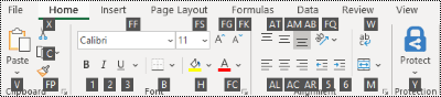
You can combine the Key Tips letters with the Alt key to make shortcuts called Access Keys for the ribbon options. For example, press Alt+H to open the Home tab, and Alt+Q to move to the Tell me or Search field. Press Alt again to see KeyTips for the options for the selected tab.
Depending on the version of Microsoft 365 you are using, the Search text field at the top of the app window might be called Tell Me instead. Both offer a largely similar experience, but some options and search results can vary.
In Office 2013 and Office 2010, most of the old Alt key menu shortcuts still work, too. However, you need to know the full shortcut. For example, press Alt, and then press one of the old menu keys, for example, E (Edit), V (View), I (Insert), and so on. A notification pops up saying you’re using an access key from an earlier version of Microsoft 365. If you know the entire key sequence, go ahead, and use it. If you don’t know the sequence, press Esc and use Key Tips instead.
Use the Access keys for ribbon tabs
To go directly to a tab on the ribbon, press one of the following access keys. Additional tabs might appear depending on your selection in the worksheet.
|
To do this |
Press |
|---|---|
|
Move to the Tell me or Search field on the ribbon and type a search term for assistance or Help content. |
Alt+Q, then enter the search term. |
|
Open the File menu. |
Alt+F |
|
Open the Home tab and format text and numbers and use the Find tool. |
Alt+H |
|
Open the Insert tab and insert PivotTables, charts, add-ins, Sparklines, pictures, shapes, headers, or text boxes. |
Alt+N |
|
Open the Page Layout tab and work with themes, page setup, scale, and alignment. |
Alt+P |
|
Open the Formulas tab and insert, trace, and customize functions and calculations. |
Alt+M |
|
Open the Data tab and connect to, sort, filter, analyze, and work with data. |
Alt+A |
|
Open the Review tab and check spelling, add notes and threaded comments, and protect sheets and workbooks. |
Alt+R |
|
Open the View tab and preview page breaks and layouts, show and hide gridlines and headings, set zoom magnification, manage windows and panes, and view macros. |
Alt+W |
Top of Page
Work in the ribbon with the keyboard
|
To do this |
Press |
|---|---|
|
Select the active tab on the ribbon and activate the access keys. |
Alt or F10. To move to a different tab, use access keys or the arrow keys. |
|
Move the focus to commands on the ribbon. |
Tab key or Shift+Tab |
|
Move down, up, left, or right, respectively, among the items on the ribbon. |
Arrow keys |
|
Show the tooltip for the ribbon element currently in focus. |
Ctrl+Shift+F10 |
|
Activate a selected button. |
Spacebar or Enter |
|
Open the list for a selected command. |
Down arrow key |
|
Open the menu for a selected button. |
Alt+Down arrow key |
|
When a menu or submenu is open, move to the next command. |
Down arrow key |
|
Expand or collapse the ribbon. |
Ctrl+F1 |
|
Open a context menu. |
Shift+F10 Or, on a Windows keyboard, the Windows Menu key (usually between the Alt Gr and right Ctrl keys) |
|
Move to the submenu when a main menu is open or selected. |
Left arrow key |
|
Move from one group of controls to another. |
Ctrl+Left or Right arrow key |
Top of Page
Keyboard shortcuts for navigating in cells
|
To do this |
Press |
|---|---|
|
Move to the previous cell in a worksheet or the previous option in a dialog box. |
Shift+Tab |
|
Move one cell up in a worksheet. |
Up arrow key |
|
Move one cell down in a worksheet. |
Down arrow key |
|
Move one cell left in a worksheet. |
Left arrow key |
|
Move one cell right in a worksheet. |
Right arrow key |
|
Move to the edge of the current data region in a worksheet. |
Ctrl+Arrow key |
|
Enter the End mode, move to the next nonblank cell in the same column or row as the active cell, and turn off End mode. If the cells are blank, move to the last cell in the row or column. |
End, Arrow key |
|
Move to the last cell on a worksheet, to the lowest used row of the rightmost used column. |
Ctrl+End |
|
Extend the selection of cells to the last used cell on the worksheet (lower-right corner). |
Ctrl+Shift+End |
|
Move to the cell in the upper-left corner of the window when Scroll lock is turned on. |
Home+Scroll lock |
|
Move to the beginning of a worksheet. |
Ctrl+Home |
|
Move one screen down in a worksheet. |
Page down |
|
Move to the next sheet in a workbook. |
Ctrl+Page down |
|
Move one screen to the right in a worksheet. |
Alt+Page down |
|
Move one screen up in a worksheet. |
Page up |
|
Move one screen to the left in a worksheet. |
Alt+Page up |
|
Move to the previous sheet in a workbook. |
Ctrl+Page up |
|
Move one cell to the right in a worksheet. Or, in a protected worksheet, move between unlocked cells. |
Tab key |
|
Open the list of validation choices on a cell that has data validation option applied to it. |
Alt+Down arrow key |
|
Cycle through floating shapes, such as text boxes or images. |
Ctrl+Alt+5, then the Tab key repeatedly |
|
Exit the floating shape navigation and return to the normal navigation. |
Esc |
|
Scroll horizontally. |
Ctrl+Shift, then scroll your mouse wheel up to go left, down to go right |
|
Zoom in. |
Ctrl+Alt+Equal sign ( = ) |
|
Zoom out. |
Ctrl+Alt+Minus sign (-) |
Top of Page
Keyboard shortcuts for formatting cells
|
To do this |
Press |
|---|---|
|
Open the Format Cells dialog box. |
Ctrl+1 |
|
Format fonts in the Format Cells dialog box. |
Ctrl+Shift+F or Ctrl+Shift+P |
|
Edit the active cell and put the insertion point at the end of its contents. Or, if editing is turned off for the cell, move the insertion point into the formula bar. If editing a formula, toggle Point mode off or on so you can use the arrow keys to create a reference. |
F2 |
|
Insert a note. Open and edit a cell note. |
Shift+F2 Shift+F2 |
|
Insert a threaded comment. Open and reply to a threaded comment. |
Ctrl+Shift+F2 Ctrl+Shift+F2 |
|
Open the Insert dialog box to insert blank cells. |
Ctrl+Shift+Plus sign (+) |
|
Open the Delete dialog box to delete selected cells. |
Ctrl+Minus sign (-) |
|
Enter the current time. |
Ctrl+Shift+Colon (:) |
|
Enter the current date. |
Ctrl+Semicolon (;) |
|
Switch between displaying cell values or formulas in the worksheet. |
Ctrl+Grave accent (`) |
|
Copy a formula from the cell above the active cell into the cell or the formula bar. |
Ctrl+Apostrophe (‘) |
|
Move the selected cells. |
Ctrl+X |
|
Copy the selected cells. |
Ctrl+C |
|
Paste content at the insertion point, replacing any selection. |
Ctrl+V |
|
Open the Paste Special dialog box. |
Ctrl+Alt+V |
|
Italicize text or remove italic formatting. |
Ctrl+I or Ctrl+3 |
|
Bold text or remove bold formatting. |
Ctrl+B or Ctrl+2 |
|
Underline text or remove underline. |
Ctrl+U or Ctrl+4 |
|
Apply or remove strikethrough formatting. |
Ctrl+5 |
|
Switch between hiding objects, displaying objects, and displaying placeholders for objects. |
Ctrl+6 |
|
Apply an outline border to the selected cells. |
Ctrl+Shift+Ampersand sign (&) |
|
Remove the outline border from the selected cells. |
Ctrl+Shift+Underscore (_) |
|
Display or hide the outline symbols. |
Ctrl+8 |
|
Use the Fill Down command to copy the contents and format of the topmost cell of a selected range into the cells below. |
Ctrl+D |
|
Apply the General number format. |
Ctrl+Shift+Tilde sign (~) |
|
Apply the Currency format with two decimal places (negative numbers in parentheses). |
Ctrl+Shift+Dollar sign ($) |
|
Apply the Percentage format with no decimal places. |
Ctrl+Shift+Percent sign (%) |
|
Apply the Scientific number format with two decimal places. |
Ctrl+Shift+Caret sign (^) |
|
Apply the Date format with the day, month, and year. |
Ctrl+Shift+Number sign (#) |
|
Apply the Time format with the hour and minute, and AM or PM. |
Ctrl+Shift+At sign (@) |
|
Apply the Number format with two decimal places, thousands separator, and minus sign (-) for negative values. |
Ctrl+Shift+Exclamation point (!) |
|
Open the Insert hyperlink dialog box. |
Ctrl+K |
|
Check spelling in the active worksheet or selected range. |
F7 |
|
Display the Quick Analysis options for selected cells that contain data. |
Ctrl+Q |
|
Display the Create Table dialog box. |
Ctrl+L or Ctrl+T |
|
Open the Workbook Statistics dialog box. |
Ctrl+Shift+G |
Top of Page
Keyboard shortcuts in the Paste Special dialog box in Excel 2013
In Excel 2013, you can paste a specific aspect of the copied data like its formatting or value using the Paste Special options. After you’ve copied the data, press Ctrl+Alt+V, or Alt+E+S to open the Paste Special dialog box.
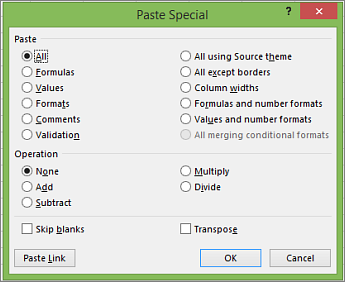
Tip: You can also select Home > Paste > Paste Special.
To pick an option in the dialog box, press the underlined letter for that option. For example, press the letter C to pick the Comments option.
|
To do this |
Press |
|---|---|
|
Paste all cell contents and formatting. |
A |
|
Paste only the formulas as entered in the formula bar. |
F |
|
Paste only the values (not the formulas). |
V |
|
Paste only the copied formatting. |
T |
|
Paste only comments and notes attached to the cell. |
C |
|
Paste only the data validation settings from copied cells. |
N |
|
Paste all cell contents and formatting from copied cells. |
H |
|
Paste all cell contents without borders. |
X |
|
Paste only column widths from copied cells. |
W |
|
Paste only formulas and number formats from copied cells. |
R |
|
Paste only the values (not formulas) and number formats from copied cells. |
U |
Top of Page
Keyboard shortcuts for making selections and performing actions
|
To do this |
Press |
|---|---|
|
Select the entire worksheet. |
Ctrl+A or Ctrl+Shift+Spacebar |
|
Select the current and next sheet in a workbook. |
Ctrl+Shift+Page down |
|
Select the current and previous sheet in a workbook. |
Ctrl+Shift+Page up |
|
Extend the selection of cells by one cell. |
Shift+Arrow key |
|
Extend the selection of cells to the last nonblank cell in the same column or row as the active cell, or if the next cell is blank, to the next nonblank cell. |
Ctrl+Shift+Arrow key |
|
Turn extend mode on and use the arrow keys to extend a selection. Press again to turn off. |
F8 |
|
Add a non-adjacent cell or range to a selection of cells by using the arrow keys. |
Shift+F8 |
|
Start a new line in the same cell. |
Alt+Enter |
|
Fill the selected cell range with the current entry. |
Ctrl+Enter |
|
Complete a cell entry and select the cell above. |
Shift+Enter |
|
Select an entire column in a worksheet. |
Ctrl+Spacebar |
|
Select an entire row in a worksheet. |
Shift+Spacebar |
|
Select all objects on a worksheet when an object is selected. |
Ctrl+Shift+Spacebar |
|
Extend the selection of cells to the beginning of the worksheet. |
Ctrl+Shift+Home |
|
Select the current region if the worksheet contains data. Press a second time to select the current region and its summary rows. Press a third time to select the entire worksheet. |
Ctrl+A or Ctrl+Shift+Spacebar |
|
Select the current region around the active cell. |
Ctrl+Shift+Asterisk sign (*) |
|
Select the first command on the menu when a menu or submenu is visible. |
Home |
|
Repeat the last command or action, if possible. |
Ctrl+Y |
|
Undo the last action. |
Ctrl+Z |
|
Expand grouped rows or columns. |
While hovering over the collapsed items, press and hold the Shift key and scroll down. |
|
Collapse grouped rows or columns. |
While hovering over the expanded items, press and hold the Shift key and scroll up. |
Top of Page
Keyboard shortcuts for working with data, functions, and the formula bar
|
To do this |
Press |
|---|---|
|
Turn on or off tooltips for checking formulas directly in the formula bar or in the cell you’re editing. |
Ctrl+Alt+P |
|
Edit the active cell and put the insertion point at the end of its contents. Or, if editing is turned off for the cell, move the insertion point into the formula bar. If editing a formula, toggle Point mode off or on so you can use the arrow keys to create a reference. |
F2 |
|
Expand or collapse the formula bar. |
Ctrl+Shift+U |
|
Cancel an entry in the cell or formula bar. |
Esc |
|
Complete an entry in the formula bar and select the cell below. |
Enter |
|
Move the cursor to the end of the text when in the formula bar. |
Ctrl+End |
|
Select all text in the formula bar from the cursor position to the end. |
Ctrl+Shift+End |
|
Calculate all worksheets in all open workbooks. |
F9 |
|
Calculate the active worksheet. |
Shift+F9 |
|
Calculate all worksheets in all open workbooks, regardless of whether they have changed since the last calculation. |
Ctrl+Alt+F9 |
|
Check dependent formulas, and then calculate all cells in all open workbooks, including cells not marked as needing to be calculated. |
Ctrl+Alt+Shift+F9 |
|
Display the menu or message for an Error Checking button. |
Alt+Shift+F10 |
|
Display the Function Arguments dialog box when the insertion point is to the right of a function name in a formula. |
Ctrl+A |
|
Insert argument names and parentheses when the insertion point is to the right of a function name in a formula. |
Ctrl+Shift+A |
|
Insert the AutoSum formula |
Alt+Equal sign ( = ) |
|
Invoke Flash Fill to automatically recognize patterns in adjacent columns and fill the current column |
Ctrl+E |
|
Cycle through all combinations of absolute and relative references in a formula if a cell reference or range is selected. |
F4 |
|
Insert a function. |
Shift+F3 |
|
Copy the value from the cell above the active cell into the cell or the formula bar. |
Ctrl+Shift+Straight quotation mark («) |
|
Create an embedded chart of the data in the current range. |
Alt+F1 |
|
Create a chart of the data in the current range in a separate Chart sheet. |
F11 |
|
Define a name to use in references. |
Alt+M, M, D |
|
Paste a name from the Paste Name dialog box (if names have been defined in the workbook). |
F3 |
|
Move to the first field in the next record of a data form. |
Enter |
|
Create, run, edit, or delete a macro. |
Alt+F8 |
|
Open the Microsoft Visual Basic For Applications Editor. |
Alt+F11 |
|
Open the Power Query Editor |
Alt+F12 |
Top of Page
Keyboard shortcuts for refreshing external data
Use the following keys to refresh data from external data sources.
|
To do this |
Press |
|---|---|
|
Stop a refresh operation. |
Esc |
|
Refresh data in the current worksheet. |
Ctrl+F5 |
|
Refresh all data in the workbook. |
Ctrl+Alt+F5 |
Top of Page
Power Pivot keyboard shortcuts
Use the following keyboard shortcuts with Power Pivot in Microsoft 365, Excel 2019, Excel 2016, and Excel 2013.
|
To do this |
Press |
|---|---|
|
Open the context menu for the selected cell, column, or row. |
Shift+F10 |
|
Select the entire table. |
Ctrl+A |
|
Copy selected data. |
Ctrl+C |
|
Delete the table. |
Ctrl+D |
|
Move the table. |
Ctrl+M |
|
Rename the table. |
Ctrl+R |
|
Save the file. |
Ctrl+S |
|
Redo the last action. |
Ctrl+Y |
|
Undo the last action. |
Ctrl+Z |
|
Select the current column. |
Ctrl+Spacebar |
|
Select the current row. |
Shift+Spacebar |
|
Select all cells from the current location to the last cell of the column. |
Shift+Page down |
|
Select all cells from the current location to the first cell of the column. |
Shift+Page up |
|
Select all cells from the current location to the last cell of the row. |
Shift+End |
|
Select all cells from the current location to the first cell of the row. |
Shift+Home |
|
Move to the previous table. |
Ctrl+Page up |
|
Move to the next table. |
Ctrl+Page down |
|
Move to the first cell in the upper-left corner of selected table. |
Ctrl+Home |
|
Move to the last cell in the lower-right corner of selected table. |
Ctrl+End |
|
Move to the first cell of the selected row. |
Ctrl+Left arrow key |
|
Move to the last cell of the selected row. |
Ctrl+Right arrow key |
|
Move to the first cell of the selected column. |
Ctrl+Up arrow key |
|
Move to the last cell of selected column. |
Ctrl+Down arrow key |
|
Close a dialog box or cancel a process, such as a paste operation. |
Ctrl+Esc |
|
Open the AutoFilter Menu dialog box. |
Alt+Down arrow key |
|
Open the Go To dialog box. |
F5 |
|
Recalculate all formulas in the Power Pivot window. For more information, see Recalculate Formulas in Power Pivot. |
F9 |
Top of Page
Function keys
|
Key |
Description |
|---|---|
|
F1 |
|
|
F2 |
|
|
F3 |
|
|
F4 |
|
|
F5 |
|
|
F6 |
|
|
F7 |
|
|
F8 |
|
|
F9 |
|
|
F10 |
|
|
F11 |
|
|
F12 |
|
Top of Page
Other useful shortcut keys
|
Key |
Description |
|---|---|
|
Alt |
For example,
|
|
Arrow keys |
|
|
Backspace |
|
|
Delete |
|
|
End |
|
|
Enter |
|
|
Esc |
|
|
Home |
|
|
Page down |
|
|
Page up |
|
|
Shift |
|
|
Spacebar |
|
|
Tab key |
|
Top of Page
See also
Excel help & learning
Basic tasks using a screen reader with Excel
Use a screen reader to explore and navigate Excel
Screen reader support for Excel
This article describes the keyboard shortcuts, function keys, and some other common shortcut keys in Excel for Mac.
Notes:
-
The settings in some versions of the Mac operating system (OS) and some utility applications might conflict with keyboard shortcuts and function key operations in Microsoft 365 for Mac.
-
If you don’t find a keyboard shortcut here that meets your needs, you can create a custom keyboard shortcut. For instructions, go to Create a custom keyboard shortcut for Office for Mac.
-
Many of the shortcuts that use the Ctrl key on a Windows keyboard also work with the Control key in Excel for Mac. However, not all do.
-
To quickly find a shortcut in this article, you can use the Search. Press
+F, and then type your search words. -
Click-to-add is available but requires a setup. Select Excel> Preferences > Edit > Enable Click to Add Mode. To start a formula, type an equal sign ( = ), and then select cells to add them together. The plus sign (+) will be added automatically.
 +F, and then type your search words.
In this topic
-
Frequently used shortcuts
-
Shortcut conflicts
-
Change system preferences for keyboard shortcuts with the mouse
-
-
Work in windows and dialog boxes
-
Move and scroll in a sheet or workbook
-
Enter data on a sheet
-
Work in cells or the Formula bar
-
Format and edit data
-
Select cells, columns, or rows
-
Work with a selection
-
Use charts
-
Sort, filter, and use PivotTable reports
-
Outline data
-
Use function key shortcuts
-
Change function key preferences with the mouse
-
-
Drawing
Frequently used shortcuts
This table itemizes the most frequently used shortcuts in Excel for Mac.
|
To do this |
Press |
|---|---|
|
Paste selection. |
|
|
Copy selection. |
|
|
Clear selection. |
Delete |
|
Save workbook. |
|
|
Undo action. |
|
|
Redo action. |
|
|
Cut selection. |
|
|
Apply bold formatting. |
|
|
Print workbook. |
|
|
Open Visual Basic. |
Option+F11 |
|
Fill cells down. |
|
|
Fill cells right. |
|
|
Insert cells. |
Control+Shift+Equal sign ( = ) |
|
Delete cells. |
|
|
Calculate all open workbooks. |
|
|
Close window. |
|
|
Quit Excel. |
|
|
Display the Go To dialog box. |
Control+G |
|
Display the Format Cells dialog box. |
|
|
Display the Replace dialog box. |
Control+H |
|
Use Paste Special. |
|
|
Apply underline formatting. |
|
|
Apply italic formatting. |
|
|
Open a new blank workbook. |
|
|
Create a new workbook from template. |
|
|
Display the Save As dialog box. |
|
|
Display the Help window. |
F1 |
|
Select all. |
|
|
Add or remove a filter. |
|
|
Minimize or maximize the ribbon tabs. |
|
|
Display the Open dialog box. |
|
|
Check spelling. |
F7 |
|
Open the thesaurus. |
Shift+F7 |
|
Display the Formula Builder. |
Shift+F3 |
|
Open the Define Name dialog box. |
|
|
Insert or reply to a threaded comment. |
|
|
Open the Create names dialog box. |
|
|
Insert a new sheet. * |
Shift+F11 |
|
Print preview. |
|

Top of Page
Shortcut conflicts
Some Windows keyboard shortcuts conflict with the corresponding default macOS keyboard shortcuts. This topic flags such shortcuts with an asterisk (*). To use these shortcuts, you might have to change your Mac keyboard settings to change the Show Desktop shortcut for the key.
Change system preferences for keyboard shortcuts with the mouse
-
On the Apple menu, select System Settings.
-
Select Keyboard.
-
Select Keyboard Shortcuts.
-
Find the shortcut that you want to use in Excel and clear the checkbox for it.
Top of Page
Work in windows and dialog boxes
|
To do this |
Press |
|---|---|
|
Expand or minimize the ribbon. |
|
|
Switch to full screen view. |
|
|
Switch to the next application. |
|
|
Switch to the previous application. |
Shift+ |
|
Close the active workbook window. |
|
|
Take a screenshot and save it on your desktop. |
Shift+ |
|
Minimize the active window. |
Control+F9 |
|
Maximize or restore the active window. |
Control+F10 |
|
Hide Excel. |
|
|
Move to the next box, option, control, or command. |
Tab key |
|
Move to the previous box, option, control, or command. |
Shift+Tab |
|
Exit a dialog box or cancel an action. |
Esc |
|
Perform the action assigned to the default button (the button with the bold outline). |
Return |
|
Cancel the command and close the dialog box or menu. |
Esc |
Top of Page
Move and scroll in a sheet or workbook
|
To do this |
Press |
|---|---|
|
Move one cell up, down, left, or right. |
Arrow keys |
|
Move to the edge of the current data region. |
|
|
Move to the beginning of the row. |
Home |
|
Move to the beginning of the sheet. |
Control+Home |
|
Move to the last cell in use on the sheet. |
Control+End |
|
Move down one screen. |
Page down |
|
Move up one screen. |
Page up |
|
Move one screen to the right. |
Option+Page down |
|
Move one screen to the left. |
Option+Page up |
|
Move to the next sheet in the workbook. |
Control+Page down |
|
Move to the previous sheet in the workbook. |
Control+Page down |
|
Scroll to display the active cell. |
Control+Delete |
|
Display the Go To dialog box. |
Control+G |
|
Display the Find dialog box. |
Control+F |
|
Access search (when in a cell or when a cell is selected). |
|
|
Move between unlocked cells on a protected sheet. |
Tab key |
|
Scroll horizontally. |
Shift, then scroll the mouse wheel up for left, down for right |
Tip: To use the arrow keys to move between cells in Excel for Mac 2011, you must turn Scroll Lock off. To toggle Scroll Lock off or on, press Shift+F14. Depending on the type of your keyboard, you might need to use the Control, Option, or the Command key instead of the Shift key. If you are using a MacBook, you might need to plug in a USB keyboard to use the F14 key combination.
Top of Page
Enter data on a sheet
|
To do this |
Press |
|---|---|
|
Edit the selected cell. |
F2 |
|
Complete a cell entry and move forward in the selection. |
Return |
|
Start a new line in the same cell. |
Option+Return or Control+Option+Return |
|
Fill the selected cell range with the text that you type. |
|
|
Complete a cell entry and move up in the selection. |
Shift+Return |
|
Complete a cell entry and move to the right in the selection. |
Tab key |
|
Complete a cell entry and move to the left in the selection. |
Shift+Tab |
|
Cancel a cell entry. |
Esc |
|
Delete the character to the left of the insertion point or delete the selection. |
Delete |
|
Delete the character to the right of the insertion point or delete the selection. Note: Some smaller keyboards do not have this key. |
|
|
Delete text to the end of the line. Note: Some smaller keyboards do not have this key. |
Control+ |
|
Move one character up, down, left, or right. |
Arrow keys |
|
Move to the beginning of the line. |
Home |
|
Insert a note. |
Shift+F2 |
|
Open and edit a cell note. |
Shift+F2 |
|
Insert a threaded comment. |
|
|
Open and reply to a threaded comment. |
|
|
Fill down. |
Control+D |
|
Fill to the right. |
Control+R |
|
Invoke Flash Fill to automatically recognize patterns in adjacent columns and fill the current column. |
Control+E |
|
Define a name. |
Control+L |
Top of Page
Work in cells or the Formula bar
|
To do this |
Press |
|---|---|
|
Turn on or off tooltips for checking formulas directly in the formula bar. |
Control+Option+P |
|
Edit the selected cell. |
F2 |
|
Expand or collapse the formula bar. |
Control+Shift+U |
|
Edit the active cell and then clear it or delete the preceding character in the active cell as you edit the cell contents. |
Delete |
|
Complete a cell entry. |
Return |
|
Enter a formula as an array formula. |
Shift+ |
|
Cancel an entry in the cell or formula bar. |
Esc |
|
Display the Formula Builder after you type a valid function name in a formula |
Control+A |
|
Insert a hyperlink. |
|
|
Edit the active cell and position the insertion point at the end of the line. |
Control+U |
|
Open the Formula Builder. |
Shift+F3 |
|
Calculate the active sheet. |
Shift+F9 |
|
Display the context menu. |
Shift+F10 |
|
Start a formula. |
Equal sign ( = ) |
|
Toggle the formula reference style between absolute, relative, and mixed. |
|
|
Insert the AutoSum formula. |
Shift+ |
|
Enter the date. |
Control+Semicolon (;) |
|
Enter the time. |
|
|
Copy the value from the cell above the active cell into the cell or the formula bar. |
Control+Shift+Inch mark/Straight double quote («) |
|
Alternate between displaying cell values and displaying cell formulas. |
Control+Grave accent (`) |
|
Copy a formula from the cell above the active cell into the cell or the formula bar. |
Control+Apostrophe (‘) |
|
Display the AutoComplete list. |
Option+Down arrow key |
|
Define a name. |
Control+L |
|
Open the Smart Lookup pane. |
Control+Option+ |
Top of Page
Format and edit data
|
To do this |
Press |
|---|---|
|
Edit the selected cell. |
F2 |
|
Create a table. |
|
|
Insert a line break in a cell. |
|
|
Insert special characters like symbols, including emoji. |
Control+ |
|
Increase font size. |
Shift+ |
|
Decrease font size. |
Shift+ |
|
Align center. |
|
|
Align left. |
|
|
Display the Modify Cell Style dialog box. |
Shift+ |
|
Display the Format Cells dialog box. |
|
|
Apply the general number format. |
Control+Shift+Tilde (~) |
|
Apply the currency format with two decimal places (negative numbers appear in red with parentheses). |
Control+Shift+Dollar sign ($) |
|
Apply the percentage format with no decimal places. |
Control+Shift+Percent sign (%) |
|
Apply the exponential number format with two decimal places. |
Control+Shift+Caret (^) |
|
Apply the date format with the day, month, and year. |
Control+Shift+Number sign (#) |
|
Apply the time format with the hour and minute, and indicate AM or PM. |
Control+Shift+At symbol (@) |
|
Apply the number format with two decimal places, thousands separator, and minus sign (-) for negative values. |
Control+Shift+Exclamation point (!) |
|
Apply the outline border around the selected cells. |
|
|
Add an outline border to the right of the selection. |
|
|
Add an outline border to the left of the selection. |
|
|
Add an outline border to the top of the selection. |
|
|
Add an outline border to the bottom of the selection. |
|
|
Remove outline borders. |
|
|
Apply or remove bold formatting. |
|
|
Apply or remove italic formatting. |
|
|
Apply or remove underline formatting. |
|
|
Apply or remove strikethrough formatting. |
Shift+ |
|
Hide a column. |
|
|
Unhide a column. |
Shift+ |
|
Hide a row. |
|
|
Unhide a row. |
Shift+ |
|
Edit the active cell. |
Control+U |
|
Cancel an entry in the cell or the formula bar. |
Esc |
|
Edit the active cell and then clear it or delete the preceding character in the active cell as you edit the cell contents. |
Delete |
|
Paste text into the active cell. |
|
|
Complete a cell entry |
Return |
|
Give selected cells the current cell’s entry. |
|
|
Enter a formula as an array formula. |
Shift+ |
|
Display the Formula Builder after you type a valid function name in a formula. |
Control+A |
Top of Page
Select cells, columns, or rows
|
To do this |
Press |
|---|---|
|
Extend the selection by one cell. |
Shift+Arrow key |
|
Extend the selection to the last nonblank cell in the same column or row as the active cell. |
Shift+ |
|
Extend the selection to the beginning of the row. |
Shift+Home |
|
Extend the selection to the beginning of the sheet. |
Control+Shift+Home |
|
Extend the selection to the last cell used |
Control+Shift+End |
|
Select the entire column. * |
Control+Spacebar |
|
Select the entire row. |
Shift+Spacebar |
|
Select the current region or entire sheet. Press more than once to expand the selection. |
|
|
Select only visible cells. |
Shift+ |
|
Select only the active cell when multiple cells are selected. |
Shift+Delete |
|
Extend the selection down one screen. |
Shift+Page down |
|
Extend the selection up one screen |
Shift+Page up |
|
Alternate between hiding objects, displaying objects, |
Control+6 |
|
Turn on the capability to extend a selection |
F8 |
|
Add another range of cells to the selection. |
Shift+F8 |
|
Select the current array, which is the array that the |
Control+Forward slash (/) |
|
Select cells in a row that don’t match the value |
Control+Backward slash () |
|
Select only cells that are directly referred to by formulas in the selection. |
Control+Shift+Left bracket ([) |
|
Select all cells that are directly or indirectly referred to by formulas in the selection. |
Control+Shift+Left brace ({) |
|
Select only cells with formulas that refer directly to the active cell. |
Control+Right bracket (]) |
|
Select all cells with formulas that refer directly or indirectly to the active cell. |
Control+Shift+Right brace (}) |
Top of Page
Work with a selection
|
To do this |
Press |
|---|---|
|
Copy a selection. |
|
|
Paste a selection. |
|
|
Cut a selection. |
|
|
Clear a selection. |
Delete |
|
Delete the selection. |
Control+Hyphen |
|
Undo the last action. |
|
|
Hide a column. |
|
|
Unhide a column. |
|
|
Hide a row. |
|
|
Unhide a row. |
|
|
Move selected rows, columns, or cells. |
Hold the Shift key while you drag a selected row, column, or selected cells to move the selected cells and drop to insert them in a new location. If you don’t hold the Shift key while you drag and drop, the selected cells will be cut from the original location and pasted to the new location (not inserted). |
|
Move from top to bottom within the selection (down). * |
Return |
|
Move from bottom to top within the selection (up). * |
Shift+Return |
|
Move from left to right within the selection, |
Tab key |
|
Move from right to left within the selection, |
Shift+Tab |
|
Move clockwise to the next corner of the selection. |
Control+Period (.) |
|
Group selected cells. |
|
|
Ungroup selected cells. |
|
* These shortcuts might move in another direction other than down or up. If you’d like to change the direction of these shortcuts using the mouse, select Excel > Preferences > Edit, and then, in After pressing Return, move selection, select the direction you want to move to.
Top of Page
Use charts
|
To do this |
Press |
|---|---|
|
Insert a new chart sheet. * |
F11 |
|
Cycle through chart object selection. |
Arrow keys |
Top of Page
Sort, filter, and use PivotTable reports
|
To do this |
Press |
|---|---|
|
Open the Sort dialog box. |
|
|
Add or remove a filter. |
|
|
Display the Filter list or PivotTable page |
Option+Down arrow key |
Top of Page
Outline data
|
To do this |
Press |
|---|---|
|
Display or hide outline symbols. |
Control+8 |
|
Hide selected rows. |
Control+9 |
|
Unhide selected rows. |
Control+Shift+Left parenthesis (() |
|
Hide selected columns. |
Control+Zero (0) |
|
Unhide selected columns. |
Control+Shift+Right parenthesis ()) |
Top of Page
Use function key shortcuts
Excel for Mac uses the function keys for common commands, including Copy and Paste. For quick access to these shortcuts, you can change your Apple system preferences, so you don’t have to press the Fn key every time you use a function key shortcut.
Note: Changing system function key preferences affects how the function keys work for your Mac, not just Excel for Mac. After changing this setting, you can still perform the special features printed on a function key. Just press the Fn key. For example, to use the F12 key to change your volume, you would press Fn+F12.
If a function key doesn’t work as you expect it to, press the Fn key in addition to the function key. If you don’t want to press the Fn key each time, you can change your Apple system preferences. For instructions, go to Change function key preferences with the mouse.
The following table provides the function key shortcuts for Excel for Mac.
|
To do this |
Press |
|---|---|
|
Display the Help window. |
F1 |
|
Edit the selected cell. |
F2 |
|
Insert a note or open and edit a cell note. |
Shift+F2 |
|
Insert a threaded comment or open and reply to a threaded comment. |
|
|
Open the Save dialog box. |
Option+F2 |
|
Open the Formula Builder. |
Shift+F3 |
|
Open the Define Name dialog box. |
|
|
Close a window or a dialog box. |
|
|
Display the Go To dialog box. |
F5 |
|
Display the Find dialog box. |
Shift+F5 |
|
Move to the Search Sheet dialog box. |
Control+F5 |
|
Switch focus between the worksheet, ribbon, task pane, and status bar. |
F6 or Shift+F6 |
|
Check spelling. |
F7 |
|
Open the thesaurus. |
Shift+F7 |
|
Extend the selection. |
F8 |
|
Add to the selection. |
Shift+F8 |
|
Display the Macro dialog box. |
Option+F8 |
|
Calculate all open workbooks. |
F9 |
|
Calculate the active sheet. |
Shift+F9 |
|
Minimize the active window. |
Control+F9 |
|
Display the context menu, or «right click» menu. |
Shift+F10 |
|
Display a pop-up menu (on object button menu), such as by clicking the button after you paste into a sheet. |
Option+Shift+F10 |
|
Maximize or restore the active window. |
Control+F10 |
|
Insert a new chart sheet.* |
F11 |
|
Insert a new sheet.* |
Shift+F11 |
|
Insert an Excel 4.0 macro sheet. |
|
|
Open Visual Basic. |
Option+F11 |
|
Display the Save As dialog box. |
F12 |
|
Display the Open dialog box. |
|
|
Open the Power Query Editor |
Option+F12 |
Top of Page
Change function key preferences with the mouse
-
On the Apple menu, select System Preferences > Keyboard.
-
On the Keyboard tab, select the checkbox for Use all F1, F2, etc. keys as standard function keys.
Drawing
|
To do this |
Press |
|---|---|
|
Toggle Drawing mode on and off. |
|
Top of Page
See also
Excel help & learning
Use a screen reader to explore and navigate Excel
Basic tasks using a screen reader with Excel
Screen reader support for Excel
This article describes the keyboard shortcuts in Excel for iOS.
Notes:
-
If you’re familiar with keyboard shortcuts on your macOS computer, the same key combinations work with Excel for iOS using an external keyboard, too.
-
To quickly find a shortcut, you can use the Search. Press
+F and then type your search words.
In this topic
-
Navigate the worksheet
-
Format and edit data
-
Work in cells or the formula bar
Navigate the worksheet
|
To do this |
Press |
|---|---|
|
Move one cell to the right. |
Tab key |
|
Move one cell up, down, left, or right. |
Arrow keys |
|
Move to the next sheet in the workbook. |
Option+Right arrow key |
|
Move to the previous sheet in the workbook. |
Option+Left arrow key |
Top of Page
Format and edit data
|
To do this |
Press |
|---|---|
|
Apply outline border. |
|
|
Remove outline border. |
|
|
Hide column(s). |
|
|
Hide row(s). |
Control+9 |
|
Unhide column(s). |
Shift+ |
|
Unhide row(s). |
Shift+Control+9 or Shift+Control+Left parenthesis (() |
Top of Page
Work in cells or the formula bar
|
To do this |
Press |
|---|---|
|
Move to the cell on the right. |
Tab key |
|
Move within cell text. |
Arrow keys |
|
Copy a selection. |
|
|
Paste a selection. |
|
|
Cut a selection. |
|
|
Undo an action. |
|
|
Redo an action. |
|
|
Apply bold formatting to the selected text. |
|
|
Apply italic formatting to the selected text. |
|
|
Underline the selected text. |
|
|
Select all. |
|
|
Select a range of cells. |
Shift+Left or Right arrow key |
|
Insert a line break within a cell. |
|
|
Move the cursor to the beginning of the current line within a cell. |
|
|
Move the cursor to the end of the current line within a cell. |
|
|
Move the cursor to the beginning of the current cell. |
|
|
Move the cursor to the end of the current cell. |
|
|
Move the cursor up by one paragraph within a cell that contains a line break. |
Option+Up arrow key |
|
Move the cursor down by one paragraph within a cell that contains a line break. |
Option+Down arrow key |
|
Move the cursor right by one word. |
Option+Right arrow key |
|
Move the cursor left by one word. |
Option+Left arrow key |
|
Insert an AutoSum formula. |
Shift+ |
Top of Page
See also
Excel help & learning
Screen reader support for Excel
Basic tasks using a screen reader with Excel
Use a screen reader to explore and navigate Excel
This article describes the keyboard shortcuts in Excel for Android.
Notes:
-
If you’re familiar with keyboard shortcuts on your Windows computer, the same key combinations work with Excel for Android using an external keyboard, too.
-
To quickly find a shortcut, you can use the Search. Press Control+F and then type your search words.
In this topic
-
Navigate the worksheet
-
Work with cells
Navigate the worksheet
|
To do this |
Press |
|---|---|
|
Move one cell to the right. |
Tab key |
|
Move one cell up, down, left, or right. |
Up, Down, Left, or Right arrow key |
Top of Page
Work with cells
|
To do this |
Press |
|---|---|
|
Save a worksheet. |
Control+S |
|
Copy a selection. |
Control+C |
|
Paste a selection. |
Control+V |
|
Cut a selection. |
Control+X |
|
Undo an action. |
Control+Z |
|
Redo an action. |
Control+Y |
|
Apply bold formatting. |
Control+B |
|
Apply italic formatting. |
Control+I |
|
Apply underline formatting. |
Control+U |
|
Select all. |
Control+A |
|
Find. |
Control+F |
|
Insert a line break within a cell. |
Alt+Enter |
Top of Page
See also
Excel help & learning
Screen reader support for Excel
Basic tasks using a screen reader with Excel
Use a screen reader to explore and navigate Excel
This article describes the keyboard shortcuts in Excel for the web.
Notes:
-
If you use Narrator with the Windows 10 Fall Creators Update, you have to turn off scan mode in order to edit documents, spreadsheets, or presentations with Microsoft 365 for the web. For more information, refer to Turn off virtual or browse mode in screen readers in Windows 10 Fall Creators Update.
-
To quickly find a shortcut, you can use the Search. Press Ctrl+F and then type your search words.
-
When you use Excel for the web, we recommend that you use Microsoft Edge as your web browser. Because Excel for the web runs in your web browser, the keyboard shortcuts are different from those in the desktop program. For example, you’ll use Ctrl+F6 instead of F6 for jumping in and out of the commands. Also, common shortcuts like F1 (Help) and Ctrl+O (Open) apply to the web browser — not Excel for the web.
In this article
-
Quick tips for using keyboard shortcuts with Excel for the web
-
Frequently used shortcuts
-
Access keys: Shortcuts for using the ribbon
-
Keyboard shortcuts for editing cells
-
Keyboard shortcuts for entering data
-
Keyboard shortcuts for editing data within a cell
-
Keyboard shortcuts for formatting cells
-
Keyboard shortcuts for moving and scrolling within worksheets
-
Keyboard shortcuts for working with objects
-
Keyboard shortcuts for working with cells, rows, columns, and objects
-
Keyboard shortcuts for moving within a selected range
-
Keyboard shortcuts for calculating data
-
Accessibility Shortcuts Menu (Alt+Shift+A)
-
Control keyboard shortcuts in Excel for the web by overriding browser keyboard shortcuts
Quick tips for using keyboard shortcuts with Excel for the web
-
To find any command quickly, press Alt+Windows logo key, Q to jump to the Search or Tell Me text field. In Search or Tell Me, type a word or the name of a command you want (available only in Editing mode). Search or Tell Me searches for related options and provides a list. Use the Up and Down arrow keys to select a command, and then press Enter.
Depending on the version of Microsoft 365 you are using, the Search text field at the top of the app window might be called Tell Me instead. Both offer a largely similar experience, but some options and search results can vary.
-
To jump to a particular cell in a workbook, use the Go To option: press Ctrl+G, type the cell reference (such as B14), and then press Enter.
-
If you use a screen reader, go to Accessibility Shortcuts Menu (Alt+Shift+A).
Frequently used shortcuts
These are the most frequently used shortcuts for Excel for the web.
Tip: To quickly create a new worksheet in Excel for the web, open your browser, type Excel.new in the address bar, and then press Enter.
|
To do this |
Press |
|---|---|
|
Go to a specific cell. |
Ctrl+G |
|
Move down. |
Page down or Down arrow key |
|
Move up. |
Page up or Up arrow key |
|
Print a workbook. |
Ctrl+P |
|
Copy selection. |
Ctrl+C |
|
Paste selection. |
Ctrl+V |
|
Cut selection. |
Ctrl+X |
|
Undo action. |
Ctrl+Z |
|
Open workbook. |
Ctrl+O |
|
Close workbook. |
Ctrl+W |
|
Open the Save As dialog box. |
Alt+F2 |
|
Use Find. |
Ctrl+F or Shift+F3 |
|
Apply bold formatting. |
Ctrl+B |
|
Open the context menu. |
|
|
Jump to Search or Tell me. |
Alt+Q |
|
Repeat Find downward. |
Shift+F4 |
|
Repeat Find upward. |
Ctrl+Shift+F4 |
|
Insert a chart. |
Alt+F1 |
|
Display the access keys (ribbon commands) on the classic ribbon when using Narrator. |
Alt+Period (.) |
Top of Page
Access keys: Shortcuts for using the ribbon
Excel for the web offers access keys, keyboard shortcuts to navigate the ribbon. If you’ve used access keys to save time on Excel for desktop computers, you’ll find access keys very similar in Excel for the web.
In Excel for the web, access keys all start with Alt+Windows logo key, then add a letter for the ribbon tab. For example, to go to the Review tab, press Alt+Windows logo key, R.
Note: To learn how to override the browser’s Alt-based ribbon shortcuts, go to Control keyboard shortcuts in Excel for the web by overriding browser keyboard shortcuts.
If you’re using Excel for the web on a Mac computer, press Control+Option to start.
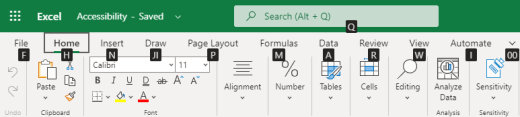
-
To get to the ribbon, press Alt+Windows logo key, or press Ctrl+F6 until you reach the Home tab.
-
To move between tabs on the ribbon, press the Tab key.
-
To hide the ribbon so you have more room to work, press Ctrl+F1. To display the ribbon again, press Ctrl+F1.
Go to the access keys for the ribbon
To go directly to a tab on the ribbon, press one of the following access keys:
|
To do this |
Press |
|---|---|
|
Go to the Search or Tell Me field on the ribbon and type a search term. |
Alt+Windows logo key, Q |
|
Open the File menu. |
Alt+Windows logo key, F |
|
Open the Home tab and format text and numbers or use other tools such as Sort & Filter. |
Alt+Windows logo key, H |
|
Open the Insert tab and insert a function, table, chart, hyperlink, or threaded comment. |
Alt+Windows logo key, N |
|
Open the Data tab and refresh connections or use data tools. |
Alt+Windows logo key, A |
|
Open the Review tab and use the Accessibility Checker or work with threaded comments and notes. |
Alt+Windows logo key, R |
|
Open the View tab to choose a view, freeze rows or columns in your worksheet, or show gridlines and headers. |
Alt+Windows logo key, W |
Top of Page
Work in the ribbon tabs and menus
The shortcuts in this table can save time when you work with the ribbon tabs and ribbon menus.
|
To do this |
Press |
|---|---|
|
Select the active tab of the ribbon and activate the access keys. |
Alt+Windows logo key. To move to a different tab, use an access key or the Tab key. |
|
Move the focus to commands on the ribbon. |
Enter, then the Tab key or Shift+Tab |
|
Activate a selected button. |
Spacebar or Enter |
|
Open the list for a selected command. |
Spacebar or Enter |
|
Open the menu for a selected button. |
Alt+Down arrow key |
|
When a menu or submenu is open, move to the next command. |
Esc |
Top of Page
Keyboard shortcuts for editing cells
Tip: If a spreadsheet opens in the Viewing mode, editing commands won’t work. To switch to Editing mode, press Alt+Windows logo key, Z, M, E.
|
To do this |
Press |
|---|---|
|
Insert a row above the current row. |
Alt+Windows logo key, H, I, R |
|
Insert a column to the left of the current column. |
Alt+Windows logo key, H, I, C |
|
Cut selection. |
Ctrl+X |
|
Copy selection. |
Ctrl+C |
|
Paste selection. |
Ctrl+V |
|
Undo an action. |
Ctrl+Z |
|
Redo an action. |
Ctrl+Y |
|
Start a new line in the same cell. |
Alt+Enter |
|
Insert a hyperlink. |
Ctrl+K |
|
Insert a table. |
Ctrl+L |
|
Insert a function. |
Shift+F3 |
|
Increase font size. |
Ctrl+Shift+Right angle bracket (>) |
|
Decrease font size. |
Ctrl+Shift+Left angle bracket (<) |
|
Apply a filter. |
Alt+Windows logo key, A, T |
|
Re-apply a filter. |
Ctrl+Alt+L |
|
Toggle AutoFilter on and off. |
Ctrl+Shift+L |
Top of Page
Keyboard shortcuts for entering data
|
To do this |
Press |
|---|---|
|
Complete cell entry and select the cell below. |
Enter |
|
Complete cell entry and select the cell above. |
Shift+Enter |
|
Complete cell entry and select the next cell in the row. |
Tab key |
|
Complete cell entry and select the previous cell in the row. |
Shift+Tab |
|
Cancel cell entry. |
Esc |
Top of Page
Keyboard shortcuts for editing data within a cell
|
To do this |
Press |
|---|---|
|
Edit the selected cell. |
F2 |
|
Cycle through all the various combinations of absolute and relative references when a cell reference or range is selected in a formula. |
F4 |
|
Clear the selected cell. |
Delete |
|
Clear the selected cell and start editing. |
Backspace |
|
Go to beginning of cell line. |
Home |
|
Go to end of cell line. |
End |
|
Select right by one character. |
Shift+Right arrow key |
|
Select to the beginning of cell data. |
Shift+Home |
|
Select to the end of cell data. |
Shift+End |
|
Select left by one character. |
Shift+Left arrow key |
|
Extend selection to the last nonblank cell in the same column or row as the active cell, or if the next cell is blank, to the next nonblank cell. |
Ctrl+Shift+Right arrow key or Ctrl+Shift+Left arrow key |
|
Insert the current date. |
Ctrl+Semicolon (;) |
|
Insert the current time. |
Ctrl+Shift+Semicolon (;) |
|
Copy a formula from the cell above. |
Ctrl+Apostrophe (‘) |
|
Copy the value from the cell above. |
Ctrl+Shift+Apostrophe (‘) |
|
Insert a formula argument. |
Ctrl+Shift+A |
Top of Page
Keyboard shortcuts for formatting cells
|
To do this |
Press |
|---|---|
|
Apply bold formatting. |
Ctrl+B |
|
Apply italic formatting. |
Ctrl+I |
|
Apply underline formatting. |
Ctrl+U |
|
Paste formatting. |
Shift+Ctrl+V |
|
Apply the outline border to the selected cells. |
Ctrl+Shift+Ampersand (&) |
|
Apply the number format. |
Ctrl+Shift+1 |
|
Apply the time format. |
Ctrl+Shift+2 |
|
Apply the date format. |
Ctrl+Shift+3 |
|
Apply the currency format. |
Ctrl+Shift+4 |
|
Apply the percentage format. |
Ctrl+Shift+5 |
|
Apply the scientific format. |
Ctrl+Shift+6 |
|
Apply outside border. |
Ctrl+Shift+7 |
|
Open the Number Format dialog box. |
Ctrl+1 |
Top of Page
Keyboard shortcuts for moving and scrolling within worksheets
|
To do this |
Press |
|---|---|
|
Move up one cell. |
Up arrow key or Shift+Enter |
|
Move down one cell. |
Down arrow key or Enter |
|
Move right one cell. |
Right arrow key or Tab key |
|
Go to the beginning of the row. |
Home |
|
Go to cell A1. |
Ctrl+Home |
|
Go to the last cell of the used range. |
Ctrl+End |
|
Move down one screen (28 rows). |
Page down |
|
Move up one screen (28 rows). |
Page up |
|
Move to the edge of the current data region. |
Ctrl+Right arrow key or Ctrl+Left arrow key |
|
Move between ribbon and workbook content. |
Ctrl+F6 |
|
Move to a different ribbon tab. |
Tab key Press Enter to go to the ribbon for the tab. |
|
Insert a new sheet. |
Shift+F11 |
|
Switch to the next sheet. |
Alt+Ctrl+Page down |
|
Switch to the next sheet (when in Microsoft Teams or a browser other than Chrome). |
Ctrl+Page down |
|
Switch to the previous sheet. |
Alt+Ctrl+Page up |
|
Switch to previous sheet (when in Microsoft Teams or a browser other than Chrome). |
Ctrl+Page up |
Top of Page
Keyboard shortcuts for working with objects
|
To do this |
Press |
|---|---|
|
Open menu or drill down. |
Alt+Down arrow key |
|
Close menu or drill up. |
Alt+Up arrow key |
|
Follow hyperlink. |
Ctrl+Enter |
|
Open a note for editing. |
Shift+F2 |
|
Open and reply to a threaded comment. |
Ctrl+Shift+F2 |
|
Rotate an object left. |
Alt+Left arrow key |
|
Rotate an object right. |
Alt+Right arrow key |
Top of Page
Keyboard shortcuts for working with cells, rows, columns, and objects
|
To do this |
Press |
|---|---|
|
Select a range of cells. |
Shift+Arrow keys |
|
Select an entire column. |
Ctrl+Spacebar |
|
Select an entire row. |
Shift+Spacebar |
|
Extend selection to the last nonblank cell in the same column or row as the active cell, or if the next cell is blank, to the next nonblank cell. |
Ctrl+Shift+Right arrow key or Ctrl+Shift+Left arrow key |
|
Add a non-adjacent cell or range to a selection. |
Shift+F8 |
|
Insert cells, rows, or columns. |
Ctrl+Plus sign (+) |
|
Delete cells, rows, or columns. |
Ctrl+Minus sign (-) |
|
Hide rows. |
Ctrl+9 |
|
Unhide rows. |
Ctrl+Shift+9 |
|
Hide columns |
Ctrl+0 |
|
Unhide columns |
Ctrl+Shift+0 |
Top of Page
Keyboard shortcuts for moving within a selected range
|
To do this |
Press |
|---|---|
|
Move from top to bottom (or forward through the selection). |
Enter |
|
Move from bottom to top (or back through the selection). |
Shift+Enter |
|
Move forward through a row (or down through a single-column selection). |
Tab key |
|
Move back through a row (or up through a single-column selection). |
Shift+Tab |
|
Move to an active cell. |
Shift+Backspace |
|
Move to an active cell and keep the selection. |
Ctrl+Backspace |
|
Rotate the active cell through the corners of the selection. |
Ctrl+Period (.) |
|
Move to the next selected range. |
Ctrl+Alt+Right arrow key |
|
Move to the previous selected range. |
Ctrl+Alt+Left arrow key |
|
Extend selection to the last used cell in the sheet. |
Ctrl+Shift+End |
|
Extend selection to the first cell in the sheet. |
Ctrl+Shift+Home |
Top of Page
Keyboard shortcuts for calculating data
|
To do this |
Press |
|---|---|
|
Calculate workbook (refresh). |
F9 |
|
Perform full calculation. |
Ctrl+Shift+Alt+F9 |
|
Refresh external data. |
Alt+F5 |
|
Refresh all external data. |
Ctrl+Alt+F5 |
|
Apply Auto Sum. |
Alt+Equal sign ( = ) |
|
Apply Flash Fill. |
Ctrl+E |
Top of Page
Accessibility Shortcuts Menu (Alt+Shift+A)
Access the common features quickly by using the following shortcuts:
|
To do this |
Press |
|---|---|
|
Cycle between landmark regions. |
Ctrl+F6 or Ctrl+Shift+F6 |
|
Move within a landmark region. |
Tab key or Shift+Tab |
|
Go to the Search or Tell Me field to run any command. |
Alt+Q |
|
Display or hide Key Tips or access the ribbon. |
Alt+Windows logo key |
|
Edit the selected cell. |
F2 |
|
Go to a specific cell. |
Ctrl+G |
|
Move to another worksheet in the workbook. |
Ctrl+Alt+Page up or Ctrl+Alt+Page down |
|
Open the context menu. |
Shift+F10 or Windows Menu key |
|
Read row header. |
Ctrl+Alt+Shift+T |
|
Read row until an active cell. |
Ctrl+Alt+Shift+Home |
|
Read row from an active cell. |
Ctrl+Alt+Shift+End |
|
Read column header. |
Ctrl+Alt+Shift+H |
|
Read column until an active cell. |
Ctrl+Alt+Shift+Page up |
|
Read column from an active cell. |
Ctrl+Alt+Shift+Page down |
|
Open a list of moving options within a dialog box. |
Ctrl+Alt+Spacebar |
Top of Page
Control keyboard shortcuts in Excel for the web by overriding browser keyboard shortcuts
Excel for the web works in a browser. Browsers have keyboard shortcuts, some of which conflict with shortcuts that work in Excel on the desktop. You can control these shortcuts, so they work the same in both versions of Excel by changing the Keyboard Shortcuts settings. Overriding browser shortcuts also enables you to open the Excel for the web Help by pressing F1.
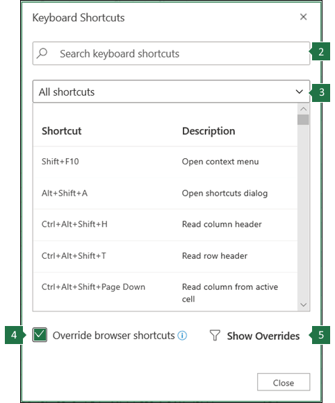
|
|
Top of Page
See also
Excel help & learning
Use a screen reader to explore and navigate Excel
Basic tasks using a screen reader with Excel
Screen reader support for Excel
Technical support for customers with disabilities
Microsoft wants to provide the best possible experience for all our customers. If you have a disability or questions related to accessibility, please contact the Microsoft Disability Answer Desk for technical assistance. The Disability Answer Desk support team is trained in using many popular assistive technologies and can offer assistance in English, Spanish, French, and American Sign Language. Please go to the Microsoft Disability Answer Desk site to find out the contact details for your region.
If you are a government, commercial, or enterprise user, please contact the enterprise Disability Answer Desk.
Toolbar or we can say it is a Quick Access Toolbar available in Excel on the left top side of the Excel window. By default, it has only a few options such as “Save,” “Redo,” and “Undo,” but we can customize the toolbar as per our choice and insert any option or button in the toolbar which will help us to reach the commands to use more quickly than before.
Table of contents
- Excel Toolbar
- How to Use the toolbar in Excel?
- Examples to Understand Quick Access Excel Toolbar
- 1 – Adding Features to the Toolbar
- Method 1
- Method 2
- Method 3
- #2 – Deleting Features from the Toolbar
- #3 – Moving the Toolbar on the Ribbon
- #4 – Modifying the Sequence of Commands and Resetting to Default Settings.
- #5 – Customize Excel Toolbar
- #6 – Exporting and Importing of Quick Access Toolbar
- 1 – Adding Features to the Toolbar
- Things to Remember
- Recommended Articles
Excel toolbar (also called Quick Access ToolbarQuick Access Toolbar (QAT) is a toolbar in Excel that may be customized and is located on the upper left-hand side of the window. It enables users to save important shortcuts and easily access them when needed.read more) is presented to access various commands to perform the operations. In addition, it is presented with an option to add or delete commands to it to access them quickly.
- Quick Access Toolbar is universal, and access is possible on any tab like “Home,” “Insert,” “Review,” “References,” etc. It is independent of the tab that we are working on simultaneously.
- It contains the various options used frequently to enhance the speed of working in Excel sheets.
- Along with the Quick Access Toolbar, another toolbar such as the “Formula Bar,” “Headings,” and Gridlines in excelGridlines are little lines made of dots to divide cells from each other in a worksheet. The gridlines have slight faint invisibility; you can find it in the page layout tab. This option has a checkbox; for activating the gridlines, you can tick on it and untick if you wish to deactivate gridlines.read more under the “Show” or “Hide” group of the “View” tab simply selecting and deselecting the checkmark shows or hides this toolbar.
- “Format” toolbar, “Drawing” toolbar, “Chart” toolbar, and “Standard” toolbar presented in the earlier version of Excel 2003 are modified into the “Home” tab and “Insert” tab in the later versions of Excel 2007 and more.
- The “Customize Quick Access Toolbar” option is available to access the full toolbars list.
You are free to use this image on your website, templates, etc, Please provide us with an attribution linkArticle Link to be Hyperlinked
For eg:
Source: Toolbar on Excel (wallstreetmojo.com)
How to Use the toolbar in Excel?
- The toolbar in Excel is used for various purposes. However, few major activities are performed on the Quick Access Toolbar on different versions of Excel.
- In the 2007 version, only three activities shift the toolbar’s location, including adding extra features or frequently used commands. In addition, deleting an element from the toolbar is possible whenever we do not want to.
- In higher versions than in 2007, the Quick Access Toolbar is used in many ways, along with adding and removing commands. These include adding commands not presented on the toolbar, modifying commands order, moving the toolbar below or above the ribbon, grouping two or more commands, exporting and importing the toolbar, customizing utilizing the “Options” command, and resetting the default settings.
- Frequent commands like “Save,” “Open,” “Redo,” “New,” “Undo,” “Email,” “Quick Print,” and print preview in excelPrint preview in Excel is a tool used to represent the print output of the current page in the excel to see if any adjustments need to be made in the final production. Print preview only displays the document on the screen, and it does not print.read more are easily added to the toolbar.
- We can select the commands not listed in the toolbar from the three categories, including “Popular Commands,” “All Commands,” and “Commands Not Listed” on the ribbon.
Examples to Understand Quick Access Excel Toolbar
Below are examples of the Excel toolbar.
1 – Adding Features to the Toolbar
Adding features or commands to the Quick Access Toolbar is essential. It is done in three ways:
- Adding commands located on the ribbon
- Adding features through the “More Commands” option
- Adding the elements presented on the different tabs directly to the toolbar
Method 1
We can add “New,” “Open,” “Save,” “Email,” “Quick Print,” and redo in excelIn Excel, we have an option named “Undo” that we may use by pressing Ctrl + Z. When we undo an action but subsequently realize it was not a mistake, we can cancel the undo action and return to the original point, using «Redo.»read more features to the toolbar. For that, select the “Customize Quick Access Toolbar” button and click on the command you want to add to the toolbar.
In the above figure, we can see the tick-marked option present in the toolbar.
Method 2
In this, a user must select the “Customize Quick Access Toolbar” in Excel and select the “More Commands” option to add the commands.
As shown in the below figure of the customize window, the user must select the commands and click on the “Add” option to add the feature to the toolbar. Added features are displayed on the excel ribbonThe ribbon is an element of the UI (User Interface) which is seen as a strip that consists of buttons or tabs; it is available at the top of the excel sheet. This option was first introduced in the Microsoft Excel 2007.read more for accessing easily.
Method 3
The user has to right-click on the feature presented on the ribbon and choose “Add to Quick Access Toolbar.”
As shown in the figure, center and right alignment commands are added to the toolbar utilizing this option.
#2 – Deleting Features from the Toolbar
To remove commands,
- Go to “More Commands.”

- Select the command that wants to be removed under the “Customize Quick Access Toolbar” option.

- Then, click on the “Remove” button to remove the selected command.

We can also do it by selecting “Excel Options” by clicking on the Microsoft office button on the top left corner of the window and then going to the “Customize” tab.
#3 – Moving the Toolbar on the Ribbon
If a user wants to shift the toolbar to another location, it is done in a few steps. First, the toolbar can be presented below or above the ribbon.
To present the toolbar below the ribbon:
- Click on the “Customize Quick Access Toolbar” button.
- Select the options shown below the ribbon.
#4 – Modifying the Sequence of Commands and Resetting to Default Settings.
The up and down buttons on the “Customize Quick Access Toolbar” present the option in the order per user. Users can discard the changes by clicking on the “Reset” option to get the default settings.
#5 – Customize Excel Toolbar
Customizing the Excel toolbar is done to add, remove, reset, change the toolbar’s location, modify, and alter the order of the features at a time.
All operations are performed quickly on the toolbar using the customization option.
#6 – Exporting and Importing of Quick Access Toolbar
Exporting and importing features are presented in the latest versions of Excel to have the same settings for files used by another computer. To do this,
- Go to “File” and select “Options.”
- Then go to a “Quick Access Toolbar.”
- Choose the “Import/Export” option to export customized settings.
Use the same steps to import customization.
Things to Remember
- The Quick Access Toolbar does not have a feature of displaying multiple lines.
- It is hard to enhance the size of the buttons to correspond to the commands. It is done only by changing the resolution of the screen.
- Another way to add commands to the toolbar is that right-clicking on the ribbon facilitates the option.
- Contents of several commands such as styles, indent, and spacing are not added to the toolbar but are represented in the form of buttons.
- Keyboard shortcutsAn Excel shortcut is a technique of performing a manual task in a quicker way.read more are also applied to the commands presented on the toolbar. For example, pressing the “ALT” key displays the shortcut numbers to utilize the commands more effectively by reducing the time.
Recommended Articles
This article is a guide to Toolbar on Excel. Here, we discuss how to add, delete, and modify features on the toolbar and how to customize the Excel toolbar. You can learn more about Excel from the following articles: –
- What does Rows Function do in Excel?
- Compare Excel Rows vs. Columns
- Analysis ToolPak in Excel
- Excel Translate
Written by Puneet for Excel 2013, Excel 2016, and Excel 2019
- It’s a collection of options for data analysis.
- You can’t add or delete options from it.
- It is not listed anywhere on the ribbon.
What is the Quick Analysis Tool?
The QUICK ANALYSIS TOOL is a collection of selected options that you can use to analyze the data quickly. It includes conditional formatting, charts, pivot table, and sparklines. It also takes care of what type of data (text, dates, or numbers) you have selected and show you the options based on that.

Quick Analysis Tool was introduced with Excel 2013, so if you are using Excel 2010 or any lower version, you won’t be able to find this option. Most of the options that you have on the quick analysis tool are fixed, but few of them are based on the selected data type.
For example, in the conditional formatting tab, you will have different options when you select dates comparing if you select numeric data. When you hover over any option from the quick analysis tool, it shows you a sneak peek at selected data.
Where the Quick Analysis Tool is Located in Excel Ribbon
The button to open the quick analysis tool is not listed anywhere on the Excel ribbon. When you select the data, Excel shows you a small icon on the bottom right side, and when you click on this icon it opens the quick analysis tool.

Quick Analysis Tool is in our list of Intermediate Excel Skills.
But I’m not Able to See the Quick Analysis Tool Button
If somehow you are not able to see a quick analysis button when you select the data (a very little chance of this), you need to check if it is disabled from the options. Go to File Tab ➜ Options ➜ General ➜ Tick Mark (Show Quick Analysis options on selection)

As I said, it was introduced in Excel 2013; if you are using any version lower than that, then you need to upgrade to the latest version.
Keyboard Shortcut to Open Quick Analysis Tool
Yes, there is a keyboard shortcut to open the quick analysis tool.
Ctrl + Q
You need to select the data, and then you need to press this keyboard shortcut.
Excel Keyboard Shortcuts Cheat Sheet
Here is one more benefit. If a quick analysis tool is disabled in the Excel options, you can still open it using the keyboard shortcut. You can also activate the quick analysis button from the right-click menu.

How to use the Quick Analysis Tool
- First, select the data you want to analyze.
- Click on the quick analysis button from the bottom right.
- Go to the tab from where you want to use the option.
- Click on the option that you want to use.
Notes
- Excel will not show you the quick analysis button if you select blank cells.
- And, if you have selected the entire column or a row.
How to use the Quick Analysis Tool for Data Analysis – Tips
1. Quickly Create Data Bars
This option comes in handy when you work with numeric data (conditional formatting data bars).

You need to click on the quick analysis button and the formatting tab and then select the “Data Bars” option. It will instantly add solid data bars (Blue) to the selected data. It is quick, right?
And if you want to change the color or want to make other customizations, go to Home Tab ➜ Styles ➜ Conditional Formatting ➜ Manage Rules.

Related: Formulas in Conditional Formatting
2. Analyze Dates with Quick Analysis Tool
If you have dates in your data, then you can quickly analyze them using the quick analysis tool. When you open it, it shows you some quick conditional formatting options to analyze dates.

- Last Month: With this option, you can highlight all the dates that are from the previous month.
- Last Week: To highlight all the dates from the previous week.
- Greater than: Highlights all the dates which are greater than the date you specify.
- Less Than: Highlights all the dates which are lower than the date specified.
- Equals To: Highlights all the dates which are equal to the date you specify.
3. Create a Pivot Table with Quick Analysis Tool
When you click on the quick analysis button and go to the tables tab, it shows you options to insert a pivot table.

Based on the data that you have selected; it shows you all the possibilities to create a pivot table. If you don’t want to go with recommendations, you can click on the more button and open the recommended PivotTables and click on the blank pivot table to create a pivot from scratch.
Related: Advanced Pivot Tables
4. Create In-Cell Charts with Sparklines
You can insert an in-cell chart using sparklines, and you can add sparklines quickly from the quick analysis tool.
- Select the data where you want to add the sparklines and click the quick analysis button.

- Go to the sparklines tab and select the type of sparkline that you want to insert.

You will instantly get the sparklines in the cells corresponding to the data that you have selected.
5. Quickly Add Grand Totals
In the totals tab, you have multiple ways to add totals, and it also gives you options for both columns and rows.

- Sum: To add a total row or column to the table.
- Average: To add an average row or column to the table.
- Count: To add an average row or column to the table.
- % Total: To add an % total row or column to the table.
- Running Total: To add a running total row or column to the table.
6. Highlight Unique and Duplicate Values
When you select text data, you will have the option to identify unique and duplicate values.

The moment you click on any of these two options, it will highlight the cells with unique or duplicate values with the red color.
If the Insert Options button isn’t visible, then go to File > Options > Advanced > in the Cut, copy and paste group, check the Show Insert Options buttons option.
Contents
- 1 How do you create an option in Excel?
- 2 How do I add options to a drop-down list in Excel?
- 3 How do I enable insert option in right click?
- 4 How do I insert a checkbox in Excel?
- 5 How do I date a picker in Excel?
- 6 How do you write an IF THEN statement in Excel?
- 7 How do I put filters on Excel?
- 8 How do I add data validation list in Excel?
- 9 How do you enter and edit data information?
- 10 Why can’t I insert anything in Excel?
- 11 Why is insert option disabled in Excel?
- 12 How do I type a checkmark?
- 13 Where is the Developer tab on Excel?
- 14 How do I automatically insert the date in Excel?
- 15 How do I insert the date and time picker control in Excel 365?
- 16 How do you do an if and formula?
- 17 How do I write a formula in Excel?
- 18 What is Ctrl I in Excel?
- 19 What is slicer in Excel?
- 20 What is Filter in Excel?
How do you create an option in Excel?
Create a drop-down list
- Select the cells that you want to contain the lists.
- On the ribbon, click DATA > Data Validation.
- In the dialog, set Allow to List.
- Click in Source, type the text or numbers (separated by commas, for a comma-delimited list) that you want in your drop-down list, and click OK.
How do I add options to a drop-down list in Excel?
Create a drop-down list
- In a new worksheet, type the entries you want to appear in your drop-down list.
- Select the cell in the worksheet where you want the drop-down list.
- Go to the Data tab on the Ribbon, then Data Validation.
- On the Settings tab, in the Allow box, click List.
How do I enable insert option in right click?
Enable Insert Button from Options
- Goto Excel File menu -> Options -> Advanced.
- Scroll to Cut,Copy, and Paste.
- Enable check box for Show Insert Options button.
- Scroll further down to “Display options for this Workbook”
- Check combobox ‘All’ under ‘For Objects, Show’
How do I insert a checkbox in Excel?
To insert a checkbox in Excel, execute these steps: On the Developer tab, in the Controls group, click Insert, and select Check Box under Form Controls. To properly position the check box, hover your mouse over it and as soon as the cursor changes to a four-pointed arrow, drag the checkbox where you want it.
How do I date a picker in Excel?
Click the Data tab. In the Insert Formula dialog box, click Insert Function. In the Categories list in the Insert Function dialog box, click Date and Time. In the Functions list, click today, and then click OK twice to return to the Date Picker Properties dialog box.
How do you write an IF THEN statement in Excel?
Use the IF function, one of the logical functions, to return one value if a condition is true and another value if it’s false. For example: =IF(A2>B2,”Over Budget”,”OK”) =IF(A2=B2,B4-A4,””)
How do I put filters on Excel?
Try it!
- Select any cell within the range.
- Select Data > Filter.
- Select the column header arrow .
- Select Text Filters or Number Filters, and then select a comparison, like Between.
- Enter the filter criteria and select OK.
How do I add data validation list in Excel?
Add data validation to a cell or a range
- Select one or more cells to validate.
- On the Data tab, in the Data Tools group, click Data Validation.
- On the Settings tab, in the Allow box, select List.
- In the Source box, type your list values, separated by commas.
- Make sure that the In-cell dropdown check box is selected.
How do you enter and edit data information?
Enter text or a number in a cell
- On the worksheet, click a cell.
- Type the numbers or text that you want to enter, and then press ENTER or TAB. To enter data on a new line within a cell, enter a line break by pressing ALT+ENTER.
Why can’t I insert anything in Excel?
Reason 2: Objects are hidden
Click “For objects, show all” within the Excel options. Within the Excel settings you can choose if objects (including charts and images) should be shown in your workbook. If this setting is set to hide all objects, you cannot insert any new objects so that the buttons are greyed-out.
Why is insert option disabled in Excel?
Why is Insert Button Disabled:
Reason 1: Excel Insert button greyed out due to Excel Sheet or Workbook is Protected. Reason 2: Excel Insert button greyed out due to Excel Sheet or Workbook is Shared.Reason 4: Excel Insert button greyed out due to Display Options for the Workbook is Disabled.
How do I type a checkmark?
Insert a check mark symbol
- In your file, place the cursor where you want to insert the symbol.
- Open the Symbol dialog box:
- In the Font box, select Wingdings.
- In the Character code box at the bottom, enter: 252.
- Select the check mark you want.
- Once the check mark has been inserted, you may change its size or color.
Where is the Developer tab on Excel?
The Developer tab isn’t displayed by default, but you can add it to the ribbon. On the File tab, go to Options > Customize Ribbon. Under Customize the Ribbon and under Main Tabs, select the Developer check box.
How do I automatically insert the date in Excel?
How to auto populate dates in Excel
- Enter your initial date in the first cell.
- Click on the cell with the first date to select it, and then drag the fill handle across or down the cells where you want Excel to add dates.
How do I insert the date and time picker control in Excel 365?
Office add-in called Mini Calendar and Date Picker via Insert Start>Options>Get add-ins, please try to check if it could meet your need and i would be happy to find out if I could help.
How do you do an if and formula?
When you combine each one of them with an IF statement, they read like this:
- AND – =IF(AND(Something is True, Something else is True), Value if True, Value if False)
- OR – =IF(OR(Something is True, Something else is True), Value if True, Value if False)
- NOT – =IF(NOT(Something is True), Value if True, Value if False)
How do I write a formula in Excel?
Create a simple formula in Excel
- On the worksheet, click the cell in which you want to enter the formula.
- Type the = (equal sign) followed by the constants and operators (up to 8192 characters) that you want to use in the calculation. For our example, type =1+1. Notes:
- Press Enter (Windows) or Return (Mac).
What is Ctrl I in Excel?
11. Ctrl + I: To italicise cell contents. 12. Ctrl + K: To insert a hyperlink in a cell.
What is slicer in Excel?
Slicers provide buttons that you can click to filter tables, or PivotTables. In addition to quick filtering, slicers also indicate the current filtering state, which makes it easy to understand what exactly is currently displayed. WindowsmacOSWeb. You can use a slicer to filter data in a table or PivotTable with ease.
What is Filter in Excel?
Filters can be used to narrow down the data in your worksheet and hide parts of it from view. While it may sound a little like grouping, filtering is different because it allows you to qualify and display only the data that interests you.