Содержание
- TODAY function
- Description
- Syntax
- Example
- How to conditionally format dates and time in Excel with formulas and inbuilt rules
- Excel conditional formatting for dates (built-in rules)
- Excel conditional formatting formulas for dates
- How to highlight weekends in Excel
- How to highlight holidays in Excel
- Conditionally format a cell when a value is changed to a date
- How to highlight rows based on a certain date in a certain column
- Conditionally format dates in Excel based on the current date
- Example 1. Highlight dates equal to, greater than or less than today
- Example 2. Conditionally format dates in Excel based on several conditions
- Example 3. Highlight upcoming dates and delays
- How to highlight dates within a date range
- How to shade gaps and time intervals
- «Days Until Next Birthday» Excel Web App
TODAY function
This article describes the formula syntax and usage of the TODAY function in Microsoft Excel.
Description
Returns the serial number of the current date. The serial number is the date-time code used by Excel for date and time calculations. If the cell format was General before the function was entered, Excel changes the cell format to Date. If you want to view the serial number, you must change the cell format to General or Number.
The TODAY function is useful when you need to have the current date displayed on a worksheet, regardless of when you open the workbook. It is also useful for calculating intervals. For example, if you know that someone was born in 1963, you might use the following formula to find that person’s age as of this year’s birthday:
This formula uses the TODAY function as an argument for the YEAR function to obtain the current year, and then subtracts 1963, returning the person’s age.
Note: If the TODAY function does not update the date when you expect it to, you might need to change the settings that control when the workbook or worksheet recalculates. On the File tab, click Options, and then in the Formulas category under Calculation options, make sure that Automatic is selected.
Syntax
The TODAY function syntax has no arguments.
Note: Excel stores dates as sequential serial numbers so they can be used in calculations. By default, January 1, 1900 is serial number 1, and January 1, 2008 is serial number 39448 because it is 39,447 days after January 1, 1900.
Example
Copy the example data in the following table, and paste it in cell A1 of a new Excel worksheet. For formulas to show results, select them, press F2, and then press Enter. If you need to, you can adjust the column widths to see all the data.
Returns the current date.
Returns the current date plus 5 days. For example, if the current date is 1/1/2012, this formula returns 1/6/2012.
Returns the number of days between the current date and 1/1/2030. Note that cell A4 must be formatted as General or Number for the result to display correctly.
Returns the current day of the month (1 — 31).
Returns the current month of the year (1 — 12). For example, if the current month is May, this formula returns 5.
Источник
How to conditionally format dates and time in Excel with formulas and inbuilt rules
 by Svetlana Cheusheva, updated on February 7, 2023
If you are a regular visitor of this blog, you’ve probably noticed a few articles covering different aspects of Excel conditional formatting. And now we will leverage this knowledge and create spreadsheets that differentiate between weekdays and weekends, highlight public holidays and display a coming deadline or delay. In other words, we are going to apply Excel conditional formatting to dates.
If you have some basic knowledge of Excel formulas, then you are most likely familiar with some of date and time functions such as NOW, TODAY, DATE, WEEKDAY, etc. In this tutorial, we are going to take this functionality a step further to conditionally format Excel dates in the way you want.
Excel conditional formatting for dates (built-in rules)
Microsoft Excel provides 10 options to format selected cells based on the current date.
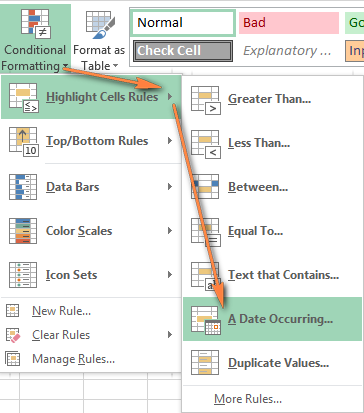
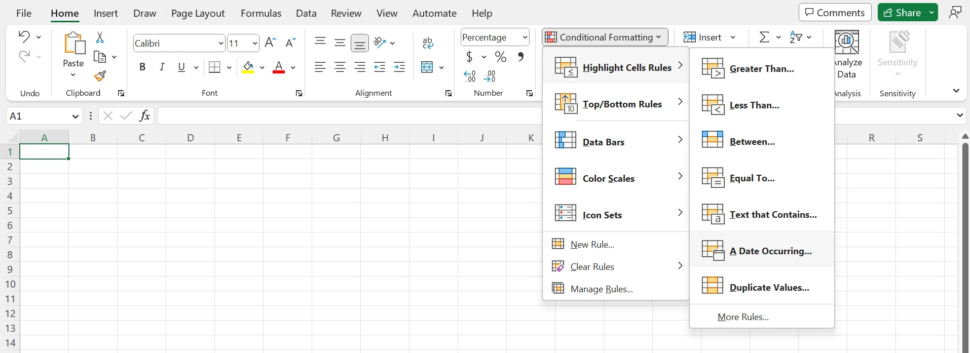
- To apply the formatting, you simply go to the Home tab >Conditional Formatting > Highlight Cell Rules and select A Date Occurring.

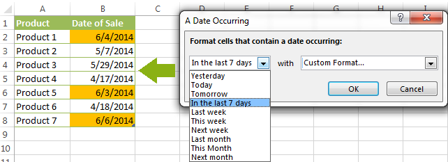
- Select one of the date options from the drop-down list in the left-hand part of the window, ranging from last month to next month.
- Finally, choose one of the pre-defined formats or set up your custom format by choosing different options on the Font, Border and Fill tabs. If the Excel standard palette does not suffice, you can always click the More colors… button.
- Click OK and enjoy the result! : )

However, this fast and straightforward way has two significant limitations — 1) it works for selected cells only and 2) the conditional format is always applied based on the current date.
Excel conditional formatting formulas for dates
If you want to highlight cells or entire rows based on a date in another cell, or create rules for greater time intervals (i.e. more than a month from the current date), you will have to create your own conditional formatting rule based on a formula. Below you will find a few examples of my favorite Excel conditional formats for dates.
How to highlight weekends in Excel
Regrettably, Microsoft Excel does not have a built-in calendar similar to Outlook’s. Well, let’s see how you can create your own automated calendar with quite little effort.
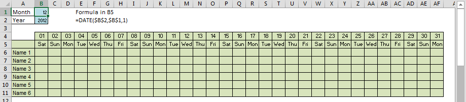
When designing your Excel calendar, you can use the =DATE(year,month,date) function to display the days of the week. Simply enter the year and the month’s number somewhere in your spreadsheet and reference those cells in the formula. Of course, you could type the numbers directly in the formula, but this is not a very efficient approach because you would have to adjust the formula for each month.
The screenshot below demonstrates the DATE function in action. I used the formula =DATE($B$2,$B$1,B$4) which is copied across row 5. 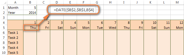
Tip. If you want to display only the days of the week like you see in the image above, select the cells with the formula (row 5 in our case), right-click and choose Format Cells…> Number > Custom. From the drop-down list under Type, select either dddd or ddd to show full day names or abbreviated names, respectively.
Your Excel calendar is almost done, and you only need to change the color of weekends. Naturally, you are not going to color the cells manually. We’ll have Excel format the weekends automatically by creating a conditional formatting rule based on the WEEKDAY formula.
- You start by selecting your Excel calendar where you want to shade the weekends. In our case, it is the range $B$4:$AE$10. Be sure to start the selection with the 1 st date column — Colum B in this example.
- On the Home tab, click Conditional Formatting menu > New Rule.
- Create a new conditional formatting rule based on a formula as explained in the above linked guide.
- In the «Format values where this formula is true» box, enter the following WEEKDAY formula that will determine which cells are Saturdays and Sundays: =WEEKDAY(B$5,2)>5
- Click the Format… button and set up your custom format by switching between the Font, Border and Fill tabs and playing with different formatting options. When done, click the OK button to preview the rule.

Now, let me briefly explain the WEEKDAY(serial_number,[return_type]) formula so that you can quickly adjust it for your own spreadsheets.
- The serial_number parameter represents the date you are trying to find. You enter a reference to your first cell with a date, B$5 in our case.
- The [return_type] parameter determines the week type (square brackets imply it is optional). You enter 2 as the return type for a week starting from Monday (1) through Sunday (7). You can find the full list of available return types here.
- Finally, you write >5 to highlight only Saturdays (6) and Sundays (7).
The screenshot below demonstrates the result in Excel 2013 — the weekends are highlighted in the reddish colour. 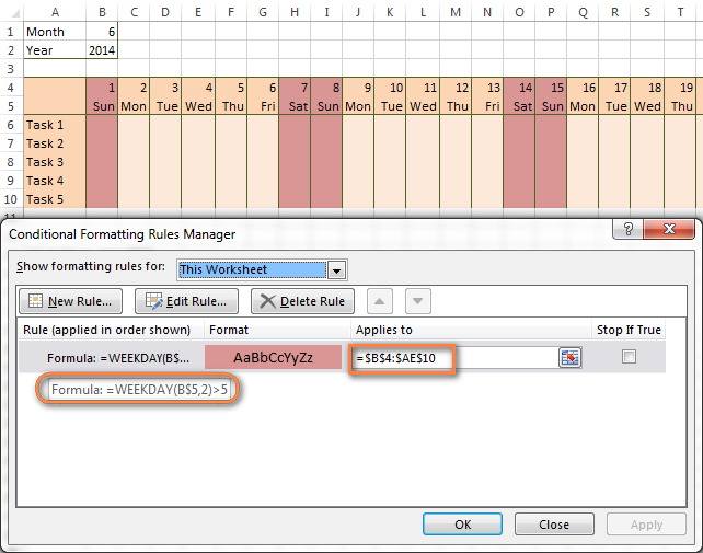
- If you have non-standard weekends in your company, e.g. Fridays and Saturdays, then you would need to tweak the formula so that it starts counting from Sunday (1) and highlight days 6 (Friday) and 7 (Saturday) — WEEKDAY(B$5,1)>5 .
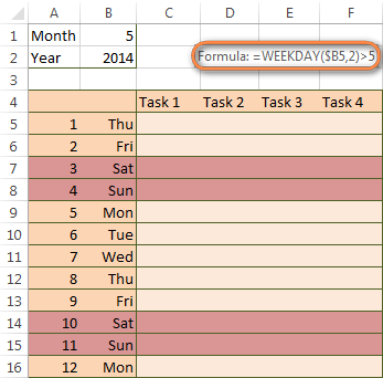
- If you are creating a horizontal (landscape) calendar, use a relative column (without $) and absolute row (with $) in a cell reference because you should lock the reference of the row — in the above example it is row 5, so we entered B$5. But if you are designing a calendar in vertical orientation, you should do the opposite, i.e. use an absolute column and relative row, e.g. $B5 as you can see in the screenshot below:
How to highlight holidays in Excel
To improve your Excel calendar further, you can shade public holidays as well. To do that, you will need to list the holidays you want to highlight in the same or some other spreadsheet.
For example, I’ve added the following holidays in column A ($A$14:$A$17). Of course, not all of them are real public holidays, but they will do for demonstration purposes : ) 
Again, you open Conditional Formatting > New Rule. In the case of holidays, you are going to use either MATCH or COUNTIF function:
Note. If you have chosen a different color for holidays, you need to move the public holiday rule to the top of the rules list via Conditional Formatting > Manage Rules…
The following image shows the result in Excel 2013: 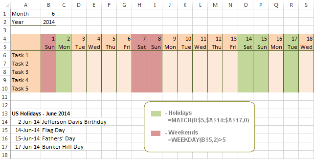
Conditionally format a cell when a value is changed to a date
It’s not a big problem to conditionally format a cell when a date is added to that cell or any other cell in the same row as long as no other value type is allowed. In this case, you could simply use a formula to highlight non-blanks, as described in Excel conditional formulas for blanks and non-blanks. But what if those cells already have some values, e.g. text, and you want to change the background color when text is changed to a date?
The task may sound a bit intricate, but the solution is very simple.
- First off, you need to determine the format code of your date. Here are just a few examples:
- D1: dd-mmm-yy or d-mmm-yy
- D2: dd-mmm or d-mmm
- D3: mmm-yy
- D4: mm/dd/yy or m/d/yy or m/d/yy h:mm
You can find the complete list of date codes in this article.
If your table contains dates in 2 or more formats, then use the OR operator, e.g. =OR(cell(«format», $A2)=»D1″, cell(«format»,$A2)=»D2″, cell(«format», $A2)=»D3″)
The screenshot below demonstrates the result of such conditional formatting rule for dates. 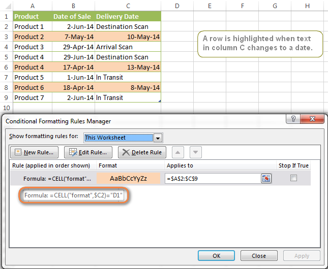
How to highlight rows based on a certain date in a certain column
Suppose, you have a large Excel spreadsheet that contains two date columns (B and C). You want to highlight every row that has a certain date, say 13-May-14, in column C.
To apply Excel conditional formatting to a certain date, you need to find its numerical value first. As you probably know, Microsoft Excel stores dates as sequential serial numbers, starting from January 1, 1900. So, 1-Jan-1900 is stored as 1, 2-Jan-1900 is stored as 2… and 13-May-14 as 41772.
To find the date’s number, right-click the cell, select Format Cells > Number and choose the General format. Write down the number you see and click Cancel because you do not really want to change the date’s format. 
That was actually the major part of the work and now you only need to create a conditional formatting rule for the entire table with this very simple formula: =$C2=41772 . The formula implies that your table has headers and row 2 is your first row with data.
An alternative way is to use the DATEVALUE formula that converts the date to the number format is which it is stored, e.g. =$C2=DATEVALUE(«5/13/2014»)
Whichever formula you use, it will have the same effect: 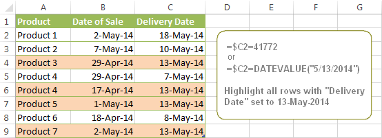
Conditionally format dates in Excel based on the current date
As you probably know Microsoft Excel provides the TODAY() functions for various calculations based on the current date. Here are just a few examples of how you can use it to conditionally format dates in Excel.
Example 1. Highlight dates equal to, greater than or less than today
To conditionally format cells or entire rows based on today’s date, you use the TODAY function as follows:
Equal to today: =$B2=TODAY()
Greater than today: =$B2>TODAY()
Less than today: =$B2
The screenshot below demonstrates the above rules in action. Please note, at the moment of writing TODAY was 12-Jun-2014. 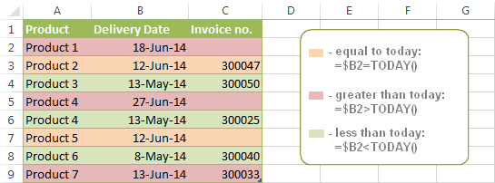
Example 2. Conditionally format dates in Excel based on several conditions
In a similar fashion, you can use the TODAY function in combination with other Excel functions to handle more complex scenarios. For example, you may want your Excel conditional formatting date formula to color the Invoice column when the Delivery Date is equal to or greater than today BUT you want the formatting to disappear when you enter the invoice number.
For this task, you would need an additional column with the following formula (where E is your Delivery column and F the Invoice column):
If the delivery date is greater than or equal to the current date and there is no number in the Invoice column, the formula returns 1, otherwise it’s 0.
After that you create a simple conditional formatting rule for the Invoice column with the formula =$G2=1 where G is your additional column. Of course, you will be able to hide this column later. 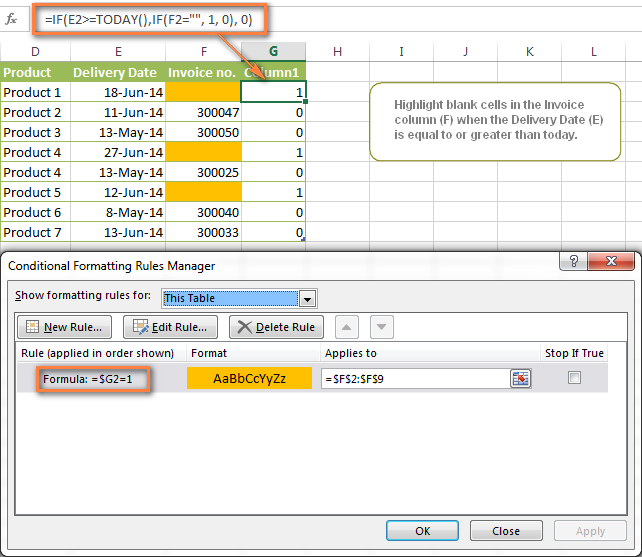
Example 3. Highlight upcoming dates and delays
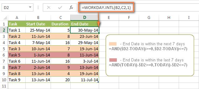
Suppose you have a project schedule in Excel that lists tasks, their start dates and durations. What you want is to have the end date for each task calculated automatically. An additional challenge is that the formula should also consider the weekends. For example, if the starting date is 13-Jun-2014 and the number of days of work (Duration) is 2, the ending date should come as 17-Jun-2014, because 14-Jun and 15-Jun are Saturday and Sunday.
To do this, we will use the WORKDAY.INTL(start_date,days,[weekend],[holidays]) function, more precisely =WORKDAY.INTL(B2,C2,1) . 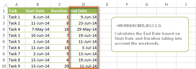
In the formula, we enter 1 as the 3 rd parameter since it indicates Saturday and Sunday as holidays. You can use another value if your weekends are different, say, Fri and Sat. The full list of the weekend values is available here. Optionally, you can also use the 4th parameter [holidays], which is a set of dates (range of cells) that should be excluded from the working day calendar.
And finally, you may want to highlight rows depending on how far away the deadline is. For example, the conditional formatting rules based on the following 2 formulas highlight upcoming and recent end dates, respectively:
- =AND($D2-TODAY()>=0,$D2-TODAY() — highlight all rows where the End Date (column D) is within the next 7 days. This formula is really handy when it comes to tracking upcoming expiration dates or payments.
- =AND(TODAY()-$D2>=0,TODAY()-$D2 — highlight all rows where the End Date (column D) is within the last 7 days. You can use this formula to track the latest overdue payments and other delays.
Here are a few more formula examples that can be applied to the table above:
=$D2 — highlights all passed dates (i.e. dates less than the current date). Can be used to format expired subscriptions, overdue payments etc.
=$D2>TODAY() — highlights all future dates (i.e. dates greater than the current date). You can use it to highlight upcoming events.
Of course, there can be infinite variations of the above formulas, depending on your particular task. For instance:
=$D2-TODAY()>=6 — highlights dates that occur in 6 or more days.
=$D2=TODAY()-14 — highlights dates occurring exactly 2 weeks ago.
How to highlight dates within a date range
If you have a long list of dates in your worksheet, you may also want to highlight the cells or rows that fall within a certain date range, i.e. highlight all dates that are between two given dates.
You can fulfil this task using the TODAY() function again. You will just have to construct a little bit more elaborate formulas as demonstrated in the examples below.
Formulas to highlight past dates
- More than 30 days ago: =TODAY()-$A2>30
- From 30 to 15 days ago, inclusive: =AND(TODAY()-$A2>=15, TODAY()-$A2
- Less than 15 days ago: =AND(TODAY()-$A2>=1, TODAY()-$A2
The current date and any future dates are not colored. 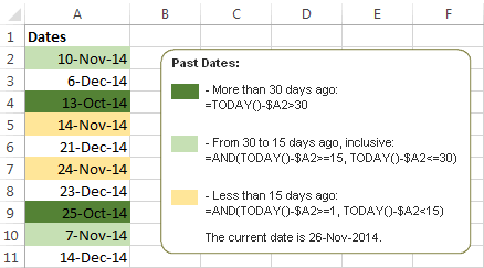
Formulas to highlight future dates
- Will occur in more than 30 days from now: =$A2-TODAY()>30
- In 30 to 15 days, inclusive: =AND($A2-TODAY()>=15, $A2-TODAY()
- In less than 15 days: =AND($A2-TODAY()>=1, $A2-TODAY()
The current date and any past dates are not colored. 
How to shade gaps and time intervals
In this last example, we are going to utilize yet another Excel date function — DATEDIF(start_date, end_date, interval) . This function calculates the difference between two dates based on the specified interval. It differs from all other functions we’ve discussed in this tutorial in the way that it lets you ignore months or years and calculate the difference only between days or months, whichever you choose.
Don’t see how this could work for you? Think about it in another way… Suppose you have a list of birthdays of your family members and friends. Would you like to know how many days there are until their next birthday? Moreover, how many days exactly are left until your wedding anniversary and other events you wouldn’t want to miss? Easily!
The formula you need is this (where A is your Date column):
=DATEDIF(TODAY(), DATE((YEAR(TODAY())+1), MONTH($A2), DAY($A2)), «yd»)
The «yd» interval type at the end of the formula is used to ignore years and calculate the difference between the days only. For the full list of available interval types, look here.
Tip. If you happen to forget or misplace that complex formula, you can use this simple one instead: =365-DATEDIF($A2,TODAY(),»yd») . It produces exactly the same results, just remember to replace 365 with 366 in leap years : )
And now let’s create an Excel conditional formatting rule to shade different gaps in different colors. In this case, it makes more sense to utilize Excel Color Scales rather than create a separate rule for each period.
The screenshot below demonstrates the result in Excel — a gradient 3-color scale with tints from green to red through yellow. 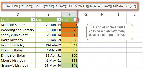
«Days Until Next Birthday» Excel Web App
We have created this Excel Web App to show you the above formula in action. Just enter your events in 1st column and change the corresponding dates in the 2nd column to experiment with the result.
Note. To view the embedded workbook, please allow marketing cookies.
If you are curious to know how to create such interactive Excel spreadsheets, check out this article on how to make web-based Excel spreadsheets.
Hopefully, at least one of the Excel conditional formats for dates discussed in this article has proven useful to you. If you are looking for a solution to some different task, you are most welcome to post a comment. Thank you for reading!
Источник
The IF function is one of the most useful Excel functions. It is used to test a condition and return one value if the condition is TRUE and another if it is FALSE.
One of the most common applications of the IF function involves the comparison of values.
These values can be numbers, text, or even dates. However, using the IF statement with date values is not as intuitive as it may seem.
In this tutorial, I will demonstrate some ways in which you can use the IF function with date values.
Syntax and Usage of the IF Function in Excel
The syntax for the IF function is as follows:
IF(logical_test, [value_if_true], [value_if_false])
Here,
- logical_test is the condition or criteria that you want the IF function to test. The result of this parameter is either TRUE or FALSE
- value_if_true is the value that you want the IF function to return if the logical_test evaluates to TRUE
- value_if_false is the value that you want the IF function to return if the logical_test evaluates to FALSE
For example, say you want to write a statement that will return the value “yes” if the value in cell reference A2 is equal to 10, and “no” if it’s anything but 10.
You can then use the following IF function for this scenario:
=IF(A2=10,"yes","no")

Comparing Dates in Excel (Using Operators)
Unlike numbers and strings, comparison operators, when used with dates, have a slightly different meaning.
Here are some of the comparison operators that you can use when comparing dates, along with what they mean:
| Operator | What it Means When Using with Dates |
|---|---|
| < | Before the given date |
| = | Same as the date with which we are comparing |
| > | After the given date |
| <= | Same as or before the given date |
| >= | Same as or after the given date |
It may look like IF formulas for dates are the same as IF functions for numeric or text values, since they use the same comparison operators.
However, it’s not as simple as that.
Unfortunately, unlike other Excel functions, the IF function cannot recognize dates.
It interprets them as regular text values.
So you cannot use a logical test such as “>05/07/2021” in your IF function, as it will simply see the value “05/07/2021” as text.
Here are a few ways in which you can incorporate date values into your IF function’s logical_test parameter.
Using the IF Function with DATEVALUE Function
If you want to use a date in your IF function’s logical test, you can wrap the date in the DATEVALUE function.
This function converts a date in text format to a serial number that Excel can recognize as a date.
If you put a date within quotes, it is essentially a text or string value.
When you pass this as a parameter to the DATEVALUE function, it takes a look at the text inside the double quotes, identifies it as a date and then converts it to an actual Excel date value.
Let us say you have a date in cell A2, and you want cell B2 to display the value “done” if the date comes before or on the same date as “05/07/2021” and display “not done” otherwise.
You can use the IF function along with DATEVALUE in cell B2 as follows:
=IF(A2<DATEVALUE("05/07/2021"),"done","not done")
Here’s a screenshot to illustrate the effect of the above formula:

Using the IF Function with the TODAY Function
If you want to compare a date with the current date, you can use the IF function with the TODAY function in the logical test.
Let’s say you have a date in cell A2 and you want cell B2 to display the value “done” if it is a date before today’s date.
If not, you want let’s say you want to display the value “not done”. You can use the IF function along with the TODAY function in cell B2 as follows:
=IF(A2<TODAY(),"done","not done")
Here’s a screenshot to illustrate the effect of the above formula (assuming the current date is 05/08/2021):

Using the IF Function with Future or Past Dates
An interesting thing about dates in Excel is that you can perform addition and subtraction operations with them too.
This is because dates are basically stored in Excel as serial numbers, starting from the date Jan 1, 1900.
Each day after that is represented by one whole number.
So, the serial number 2 corresponds to Jan 2, 1900, and so on.
This means that adding n number of days to a date is equivalent to adding the value n to the serial number that the date represents.
If TODAY() is 05/07/2021, then TODAY()+5 is five days after today, or 05/12/2021. Similarly, TODAY()-3 is three days before today or 05/04/2021.
Let’s say you have a date in cell A2 and you want cell B2 to mark it as “within range” if it is within 15 days from the current date.
If not, you want to show “out of range”. You can use the IF function along with the TODAY function in cell B2 as follows:
=IF(A2<TODAY()+15,"within range","out of range")
Here’s a screenshot to illustrate the effect of the above formula (assuming the current date is 05/08/2021):

Points to Remember
Having discussed different ways to use dates with the IF function, here are some important points to remember:
- Instead of hardcoding the dates into the IF function’s logical test parameter, you can store the date in a separate cell and refer to it with a cell reference. For example, instead of typing =IF(A2<”05/07/2021”,”done”,”not done”), you can store the date 05/07/2021 in a cell, say B2 and type the formula: =IF(A2<B2,”done”,”not done”).

- Alternatively, you can use the DATEVALUE function as explained in the first part of this tutorial.

- Another neat technique that you can use is to simply add a zero to the date (which has been enclosed in double quotes). So you can type: =IF(A2<”05/07/2021”+0,”done”,”not done”). This will make Excel take the date inside double quotes as a serial number, and use it in the logical test without having its value changed.

In this tutorial, I showed you some great techniques to use the IF function with dates. I hope the tips covered here were useful for you.
Other articles you may also like:
- Multiple If Statements in Excel (Nested Ifs, AND/OR) with Examples
- How to use Excel If Statement with Multiple Conditions Range [AND/OR]
- How to Convert Month Number to Month Name in Excel
- Why are Dates Shown as Hashtags in Excel? Easy Fix!
- How to Convert Serial Numbers to Date in Excel
- How to Get the First Day Of The Month In Excel?
Skip to content
На первый взгляд может показаться, что функцию ЕСЛИ для работы с датами можно применять так же, как для числовых и текстовых значений, которые мы только что обсудили. К сожалению, это не так.
Примеры работы функции ЕСЛИ с датами.
Дата в качестве условия, с которым работает функция ЕСЛИ, может быть записана в какую-то ячейку Excel, либо же прямо вставлена в формулу. Вот тут-то и возникают некоторые особенности и сложности работы функции ЕСЛИ с датами.
Пример 1. Формула условия для дат с
функцией ДАТАЗНАЧ (DATEVALUE)
Иногда случается, что записать дату непосредственно в функцию ЕСЛИ, не ссылаясь ни на какую ячейку. В этом случае возникают некоторые сложности.
В отличие от многих
других функций Excel, ЕСЛИ не может распознавать даты и интерпретирует их как текст,
как простые текстовые строки.
Поэтому вы не можете выразить свое логическое условие просто как >«15.07.2019» или же >15.07.2019. Увы, ни один из приведенных вариантов не верен.
Чтобы функция ЕСЛИ распознала дату в вашем логическом условии именно как дату, вы должны обернуть ее в функцию ДАТАЗНАЧ (в английском варианте – DATEVALUE).
Например, ДАТАЗНАЧ(«15.07.2019»).
Полная формула ЕСЛИ может
иметь следующую форму:
=ЕСЛИ(B2<ДАТАЗНАЧ(«10.09.2019″),»Поступил»,»Ожидается»)

Как показано на скриншоте,
эта формула ЕСЛИ оценивает даты в столбце В и возвращает «Послупил», если дата
поступления до 10 сентября. В противном случае формула возвращает «Ожидается».
Пример 2. Формула условия для дат с
функцией СЕГОДНЯ()
В случае, когда даты записаны в ячейки таблицы Excel, применять ДАТАЗНАЧ нет необходимости.
Если вы основываете свое условие на текущей дате, то можете взять функцию СЕГОДНЯ (в английском варианте — TODAY) в качестве аргумента функции ЕСЛИ.
К примеру, сегодня — 9 сентября 2019 года.
В столбце C отметим товар, который уже поступил. В ячейке C2 запишем:
=ЕСЛИ(B2<СЕГОДНЯ(),»Поступил»,»»)
В столбце D отметим товар, который еще не поступил. В ячейке D2 запишем:
=ЕСЛИ(B2<СЕГОДНЯ(),»»,»Ожидается»)

Пример 3. Расширенные
формулы ЕСЛИ для будущих и прошлых дат
Предположим, вы хотите
отметить только те даты, которые отстоят от текущей более чем на 30 дней.
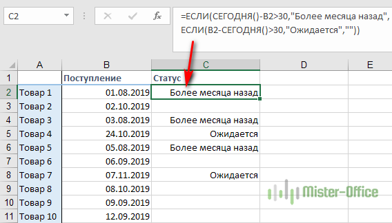
Выделим даты, отстоящие более чем на месяц от текущей, в прошлом. Укажем для них «Более месяца назад». Запишем это условие:
=ЕСЛИ(СЕГОДНЯ()-B2>30,»Более
месяца назад»,»»)
Если условие не выполнено, то в ячейку запишем пустую строку «».
А для будущих дат, также отстоящих более чем на месяц, укажем «Ожидается».
=ЕСЛИ(B2-СЕГОДНЯ()>30,»Ожидается»,»»)

Если все результаты попробовать объединить в одном столбце, то придется составить выражение с несколькими вложенными функциями ЕСЛИ:
=ЕСЛИ(СЕГОДНЯ()-B2>30,»Более месяца назад», ЕСЛИ(B2-СЕГОДНЯ()>30,»Ожидается»,»»))
Примеры работы функции ЕСЛИ:
Updated 12/16/22: Stay up to date on the latest from Excel and download Excel templates today.
Date functions in Microsoft Excel make it possible to perform date calculations, like addition or subtraction, resulting in automated or semi-automated worksheets. The NOW function, which calculates values based on the current date and time, is a great example of this.
Taking this functionality a step further, when you mix date functions with conditional formatting, you can create spreadsheets that display date alerts automatically when a deadline is near or differentiates between types of days, like weekends and weekdays.

Get a better picture of your data.
The basics of conditional formatting for dates
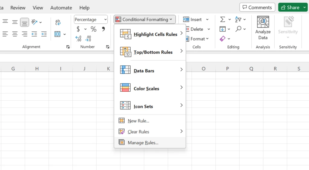
To find conditional formatting for dates, go to:
Home > Conditional Formatting > Highlight Cell Rules > A Date Occurring.
You can select the following date options, ranging from yesterday to next month:
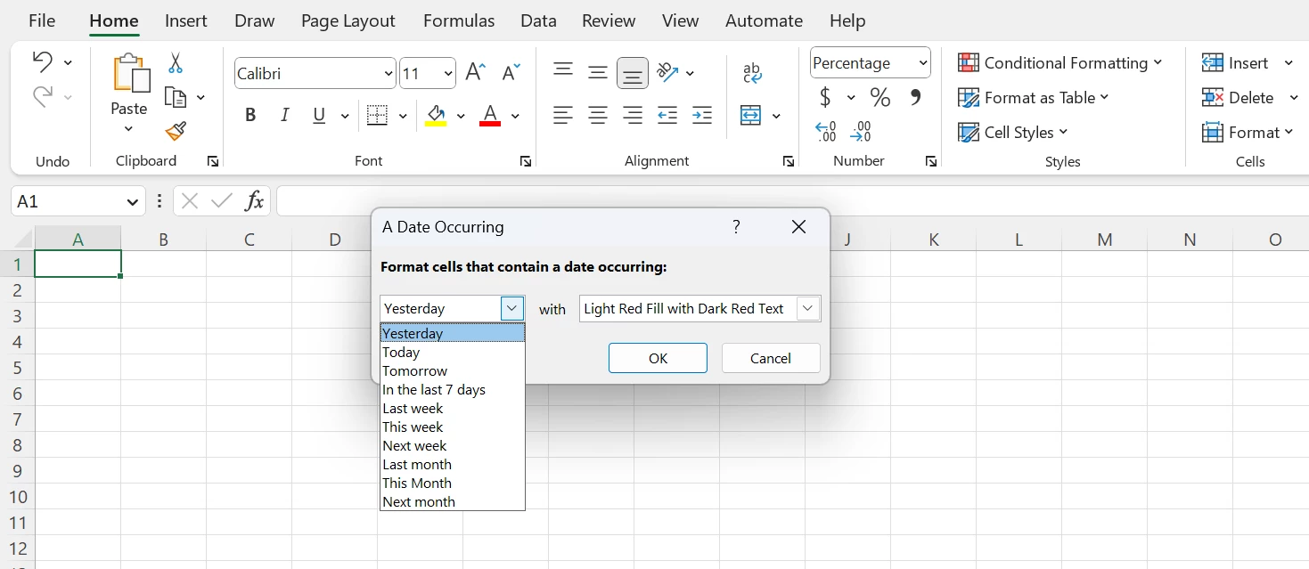
These 10 date options generate rules based on the current date. If you need to create rules for other dates (e.g., greater than a month from the current date), you can create your own new rule.
Below are step-by-step instructions for a few of my favorite conditional formats for dates.
Highlighting weekends
When you design an automated calendar you don’t need to color the weekends yourself. With the conditional formatting tool, you can automatically change the colors of weekends by basing the format on the WEEKDAY function. Assume that you have the date table—a calendar without conditional formatting:
To change the color of the weekends, open the menu Conditional Formatting > New Rule.

In the next dialog box, select the menu Use a formula to determine which cell to format.
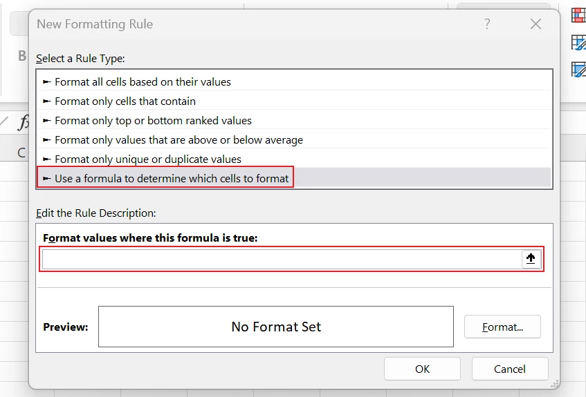
In the text box Format values where this formula is true, enter the following WEEKDAY formula to determine whether the cell is a Saturday (6) or Sunday (7):
=WEEKDAY(B$5,2)>5
Parameter 2 means Saturday = 6 and Sunday = 7. This parameter is very useful to test for weekends.
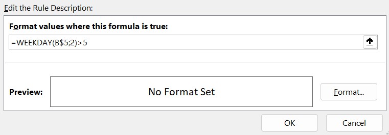
Note: In this case, you must lock the reference of the row so that the conditional format will work correctly in the other cells in this table.
Then, customize the format of your condition by clicking on the Format button and you choose a fill color (orange in this example).
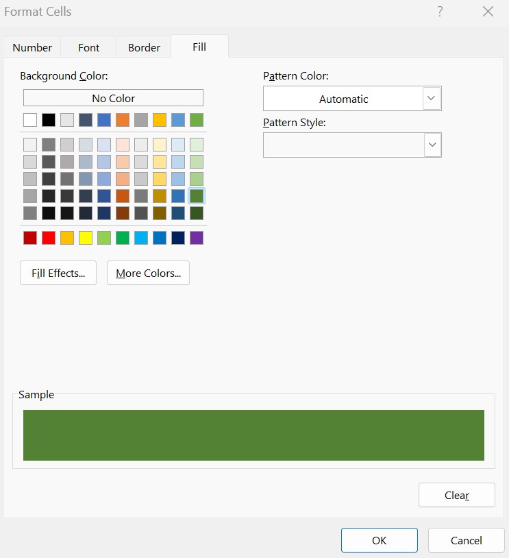
format numbers as dates <br>or times in Excel
Learn more
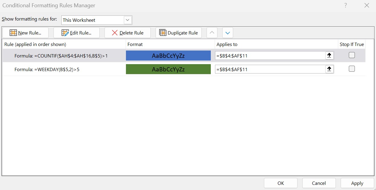
Click OK, then open Conditional Formatting> Manage Rules.
Select This Worksheet to see the worksheet rules instead of the default selection. In Applies to, change the range that corresponds to your initial selection when creating your rules to extend it to the whole column.
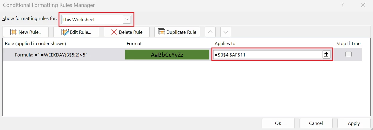
Now you will see a different color for the weekends. Note: This example shows the result in the Excel Web App.
Highlighting holidays
To enrich the previous workbook, you could also color-code holidays. To do that, you need a column with the holidays you’d like to highlight in your workbook (but not necessarily in the same sheet). In our example, we have US public holidays in column AH (as related to the year in cell B2).
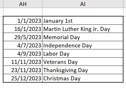
Again, open the menu Conditional Formatting > New Rule. In this case, we use the formula COUNTIF in order to count if the number of public holidays in the current month is greater than 1.
=COUNTIF($AH$4:$AH$16,B$5)>1
Then, in the dialog box Manage Rules, select the range B4:AF11. If you want to highlight the holidays over the weekends, you move the public holiday rule to the top of the list.
This example in the Excel Web App shows the result. Change the value of the month and the year to see how the calendar has a different format.
Highlighting delays
In case we want to change the color of cells based on our approach on a date again, we will use conditional formatting to make it work for us.
In the following example, we show:
- Yellow dates between 1 and 2 months.
- Orange dates between 2 and 3 months.
- Purple dates more than 3 months.
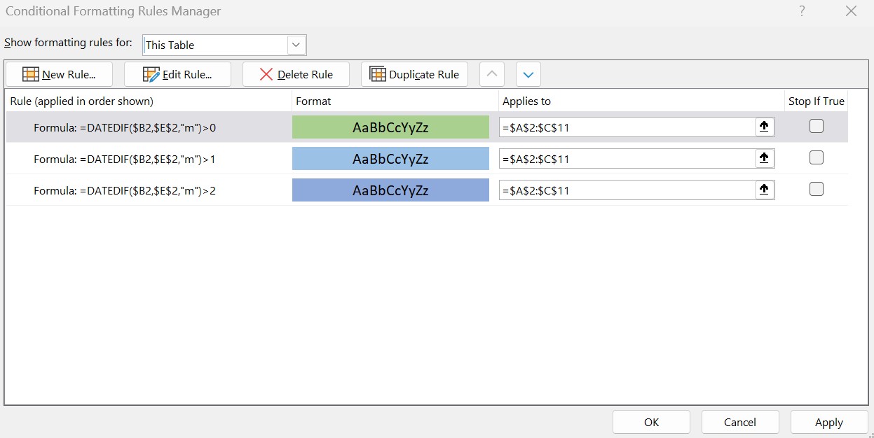
We then construct three rules of conditional formatting using the formula DATEDIF. Respectively for the three cases the following formulas:
=DATEDIF($B2,$E$2,”m”)>0
=DATEDIF($B2,$E$2,”m”)>1
=DATEDIF($B2,$E$2,”m”)>2
In the Excel Web App, try changing some dates to experiment with the result.

Task management in Microsoft 365
Collaborate on shared Office documents, including Excel, Word, and PowerPoint.
Color scales
Rather than choose a different color set for each period in our timeframe, we will work with the option of color scales to color our cells.
First, go into a new column (column E) and calculate the difference in the number of days in a year again with the DATEDIF formula and the parameter “yd”.
=DATEDIF($D2,TODAY(),”yd”)
Then choose the menu Conditional Formatting> New Rule option Format all cells based on their value and choose the following options:
- Scale = 3 colors
- Minimum = 0 Green
- Midpoint = 10 White
- Maximum = 30 Blue
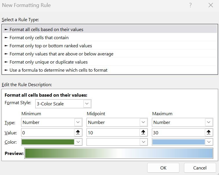
The result is a gradient color scale with nuances from green to white and through blue. The closer to 0 the more green, the closer to 10 the more white, and the closer to 30 the more blue. In the Excel app, try changing some dates to experiment with the result.
Learn more
Explore Microsoft Excel today.
Additional resources:
- Read more about the DATE function.
- Read how to format numbers as dates and times.
Return to Excel Formulas List
Download Example Workbook
Download the example workbook
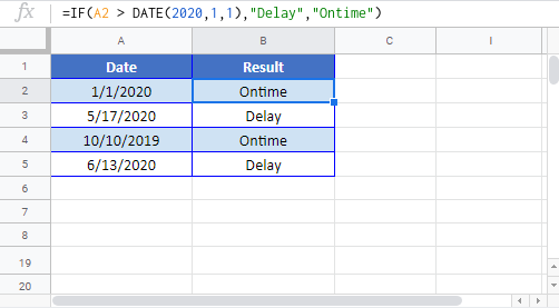
This tutorial will demonstrate how to use the IF Function with Dates in Excel and Google Sheets.
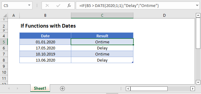
IF & DATE Functions
To use dates within IF Functions, you can use the DATE Function to define a date:
=IF(B3 > DATE(2020,1,1),"Delay","Ontime")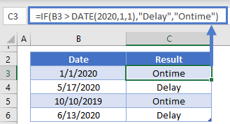
One example of this formula is to calculate if a payment is over due:
Payment Over Due
=IF(D3>=(B3+C3),"OVERDUE","ONTIME")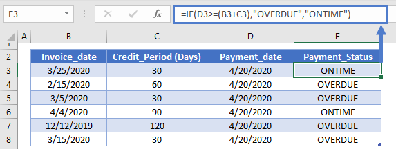
If Function with Dates – Google Sheets
All of the above examples work exactly the same in Google Sheets as in Excel.