Excel for Microsoft 365 Excel for Microsoft 365 for Mac Excel for the web Excel 2021 Excel 2021 for Mac Excel 2019 Excel 2019 for Mac Excel 2016 Excel 2016 for Mac Excel 2013 Excel 2010 Excel 2007 Excel for Mac 2011 Excel Starter 2010 More…Less
To get detailed information about a function, click its name in the first column.
Note: Version markers indicate the version of Excel a function was introduced. These functions aren’t available in earlier versions. For example, a version marker of 2013 indicates that this function is available in Excel 2013 and all later versions.
|
Function |
Description |
|---|---|
|
AND function |
Returns TRUE if all of its arguments are TRUE |
|
BYCOL function |
Applies a LAMBDA to each column and returns an array of the results |
|
BYROW function |
Applies a LAMBDA to each row and returns an array of the results |
|
FALSE function |
Returns the logical value FALSE |
|
IF function |
Specifies a logical test to perform |
|
IFERROR function |
Returns a value you specify if a formula evaluates to an error; otherwise, returns the result of the formula |
|
IFNA function |
Returns the value you specify if the expression resolves to #N/A, otherwise returns the result of the expression |
|
IFS function |
Checks whether one or more conditions are met and returns a value that corresponds to the first TRUE condition. |
|
LAMBDA function |
Create custom, reusable functions and call them by a friendly name |
|
LET function |
Assigns names to calculation results |
|
MAKEARRAY function |
Returns a calculated array of a specified row and column size, by applying a LAMBDA |
|
MAP function |
Returns an array formed by mapping each value in the array(s) to a new value by applying a LAMBDA to create a new value |
|
NOT function |
Reverses the logic of its argument |
|
OR function |
Returns TRUE if any argument is TRUE |
|
REDUCE function |
Reduces an array to an accumulated value by applying a LAMBDA to each value and returning the total value in the accumulator |
|
SCAN function |
Scans an array by applying a LAMBDA to each value and returns an array that has each intermediate value |
|
SWITCH function |
Evaluates an expression against a list of values and returns the result corresponding to the first matching value. If there is no match, an optional default value may be returned. |
|
TRUE function |
Returns the logical value TRUE |
|
XOR function |
Returns a logical exclusive OR of all arguments |
Important: The calculated results of formulas and some Excel worksheet functions may differ slightly between a Windows PC using x86 or x86-64 architecture and a Windows RT PC using ARM architecture. Learn more about the differences.
See Also
Excel functions (by category)
Excel functions (alphabetical)
Need more help?
Want more options?
Explore subscription benefits, browse training courses, learn how to secure your device, and more.
Communities help you ask and answer questions, give feedback, and hear from experts with rich knowledge.
Things will not always be the way we want them to be. The unexpected can happen. For example, let’s say you have to divide numbers. Trying to divide any number by zero (0) gives an error. Logical functions come in handy such cases. In this tutorial, we are going to cover the following topics.
In this tutorial, we are going to cover the following topics.
- What is a Logical Function?
- IF function example
- Excel Logic functions explained
- Nested IF functions
What is a Logical Function?
It is a feature that allows us to introduce decision-making when executing formulas and functions. Functions are used to;
- Check if a condition is true or false
- Combine multiple conditions together
What is a condition and why does it matter?
A condition is an expression that either evaluates to true or false. The expression could be a function that determines if the value entered in a cell is of numeric or text data type, if a value is greater than, equal to or less than a specified value, etc.
IF Function example
We will work with the home supplies budget from this tutorial. We will use the IF function to determine if an item is expensive or not. We will assume that items with a value greater than 6,000 are expensive. Those that are less than 6,000 are less expensive. The following image shows us the dataset that we will work with.
- Put the cursor focus in cell F4
- Enter the following formula that uses the IF function
=IF(E4<6000,”Yes”,”No”)
HERE,
- “=IF(…)” calls the IF functions
- “E4<6000” is the condition that the IF function evaluates. It checks the value of cell address E4 (subtotal) is less than 6,000
- “Yes” this is the value that the function will display if the value of E4 is less than 6,000
-
“No” this is the value that the function will display if the value of E4 is greater than 6,000
When you are done press the enter key
You will get the following results
Excel Logic functions explained
The following table shows all of the logical functions in Excel
| S/N | FUNCTION | CATEGORY | DESCRIPTION | USAGE |
|---|---|---|---|---|
| 01 | AND | Logical | Checks multiple conditions and returns true if they all the conditions evaluate to true. | =AND(1 > 0,ISNUMBER(1)) The above function returns TRUE because both Condition is True. |
| 02 | FALSE | Logical | Returns the logical value FALSE. It is used to compare the results of a condition or function that either returns true or false | FALSE() |
| 03 | IF | Logical |
Verifies whether a condition is met or not. If the condition is met, it returns true. If the condition is not met, it returns false. =IF(logical_test,[value_if_true],[value_if_false]) |
=IF(ISNUMBER(22),”Yes”, “No”) 22 is Number so that it return Yes. |
| 04 | IFERROR | Logical | Returns the expression value if no error occurs. If an error occurs, it returns the error value | =IFERROR(5/0,”Divide by zero error”) |
| 05 | IFNA | Logical | Returns value if #N/A error does not occur. If #N/A error occurs, it returns NA value. #N/A error means a value if not available to a formula or function. |
=IFNA(D6*E6,0) N.B the above formula returns zero if both or either D6 or E6 is/are empty |
| 06 | NOT | Logical | Returns true if the condition is false and returns false if condition is true |
=NOT(ISTEXT(0)) N.B. the above function returns true. This is because ISTEXT(0) returns false and NOT function converts false to TRUE |
| 07 | OR | Logical | Used when evaluating multiple conditions. Returns true if any or all of the conditions are true. Returns false if all of the conditions are false |
=OR(D8=”admin”,E8=”cashier”) N.B. the above function returns true if either or both D8 and E8 admin or cashier |
| 08 | TRUE | Logical | Returns the logical value TRUE. It is used to compare the results of a condition or function that either returns true or false | TRUE() |
A nested IF function is an IF function within another IF function. Nested if statements come in handy when we have to work with more than two conditions. Let’s say we want to develop a simple program that checks the day of the week. If the day is Saturday we want to display “party well”, if it’s Sunday we want to display “time to rest”, and if it’s any day from Monday to Friday we want to display, remember to complete your to do list.
A nested if function can help us to implement the above example. The following flowchart shows how the nested IF function will be implemented.
The formula for the above flowchart is as follows
=IF(B1=”Sunday”,”time to rest”,IF(B1=”Saturday”,”party well”,”to do list”))
HERE,
- “=IF(….)” is the main if function
- “=IF(…,IF(….))” the second IF function is the nested one. It provides further evaluation if the main IF function returned false.
Practical example
Create a new workbook and enter the data as shown below
- Enter the following formula
=IF(B1=”Sunday”,”time to rest”,IF(B1=”Saturday”,”party well”,”to do list”))
- Enter Saturday in cell address B1
- You will get the following results
Download the Excel file used in Tutorial
Summary
Logical functions are used to introduce decision-making when evaluating formulas and functions in Excel.
Excel Logical Functions (Table of Contents)
- Introduction to Logical Functions in Excel
- Types of Logical Functions in Excel
Introduction to Logical Functions in Excel
Logical functions in Excel work with conditions. They help deal with different situations accordingly. These functions perform work similar to IF-ELSEIF-ELSE statements in a programming language. All of these functions have simple syntaxes, and they can be beautifully combined with other functions to obtain desired results. There are various types of logical functions, some of which are commonly used in data operations in Excel.
Types of Logical Functions in Excel
The various types of logical functions in Excel are IF, IFERROR, AND, OR, NOT, TRUE, and FALSE. In the following section, we will see how to use each of them through examples.
You can download this Logical Functions Excel Template here – Logical Functions Excel Template
1. IF
It is a very simple logical function that checks if the condition to be validated as true or false. We will demonstrate the use of the IF function using a very simple example. There’s a simple dataset containing data of students and their marks. Now, if the passing marks are 40, then we would like to declare the result for each student in terms of PASS and FAIL. This can be done using the IF function.
Syntax:
Example:
Step 1: When we enter the IF function, Excel automatically pops up the list of arguments, as shown in the following screenshot.
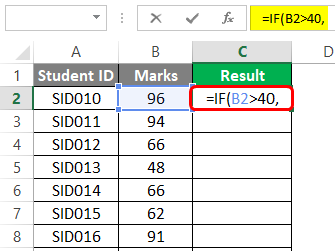
Step 2: The first argument is the logical test. In this case, the condition is that if marks are more than 40, then the result is PASS, or else it is FAIL. We passed the condition as the argument in the IF function as shown below.
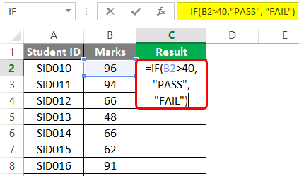
Step 3: The second and third arguments are ‘value_if_true’ and ‘value_if_false’, respectively. If marks are greater than 40, then the result should be PASS; otherwise, FAIL. This has been accomplished by passing the arguments as shown in the following screenshot.
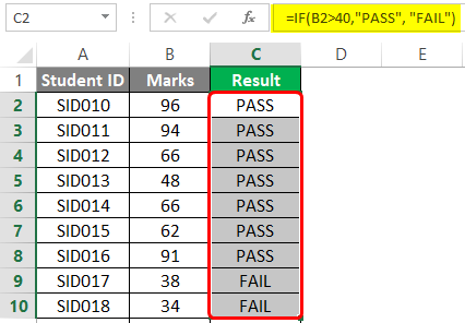
Step 4: Copy the IF function across all the required cells, and we are returned the correct result as shown in the following screenshot.
2. IFERROR
This function is used when we want to return some meaningful result in place of an error. There are various types of errors in Excel, and IFERROR is used to deal with these errors. At many times, in Excel, we are returned error values as results. In such cases, the IFERROR function becomes handy.
Syntax:
As we can see in the syntax, the IFERROR function basically means that if the value passed into it is not an error value, then that value will be given as output by the function; otherwise, the value that we have specified in ‘value if error’ argument.
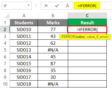
Step 1: The IFERROR function takes into consideration two arguments as seen in the syntax. This is also shown in the screenshot below.
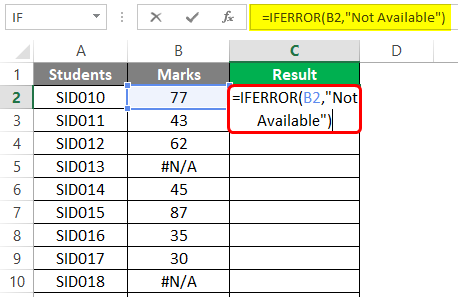
Step 2: In this example, we have marks for certain students. For some of the students, the result is not available, and for them, we have a #N/A error in the Marks column. We want this error value to be replaced with some meaningful text which is possible through the use of IFERROR. The following screenshot shows this.
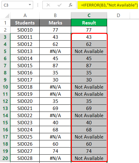
As we can see in the above screenshot, we passed marks as the first argument and kept the string “Not Available” as the second argument. It means if marks are valid, then output marks or else “Not Available”. This is as shown by the following screenshot.
3. AND
This function returns either TRUE or FALSE value by checking the conditions that are passed into it. If all the conditions passed into AND function are met, then the TRUE value is returned, and if even a single condition is not met, then the FALSE value is returned.
Syntax:
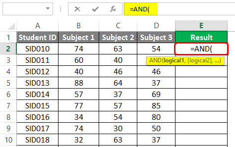
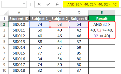
Step 1: We have marks for three different subjects for certain students. Now, we want to check if the student has passed or failed. If a student secures marks less than 40 even in a single subject out of the three subjects, he has failed in the examination. We can determine the result for each student using the AND function. When we enter the AND function, we find that arguments are highlighted. In this case, they are logical conditions, as shown below.
Step 2: Using AND, we will get results for each student by passing the conditions in the function as shown below.
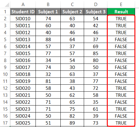
When the function is implemented, we get the result as shown below. Note, here, TRUE means pass, and FALSE means fail.
4. OR
It returns TRUE value even if a single condition out of the total conditions passed into it is met. It returns FALSE when all the arguments are FALSE.
Syntax:
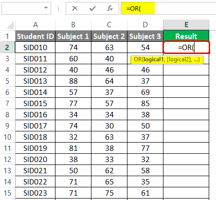
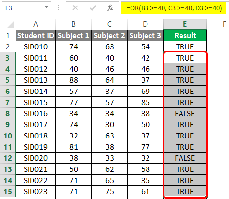
Step 1: We have marks for three different subjects for certain students. Now, if a student has secured 40 marks in at least one of the three subjects, then the result should be pass or else fail. When we enter the OR function, the arguments are highlighted as below.
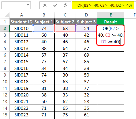
Step 2: The desired criteria for determining a student’s result can be met using the OR function as shown below.
When the above step is followed, we get the desired result, as shown below. Observe it.
5. NOT
It reverses the logical value, i.e. TRUE to FALSE and FALSE to TRUE. It is implemented usually in context-based situations.
Syntax: NOT(logical)
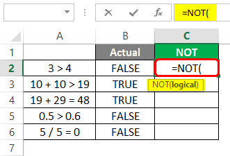
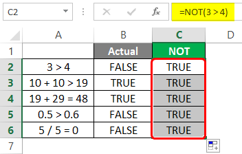
Step 1: We pass certain logical conditions into NOT and check how the function works. Have a look at the following screenshot.
The actual result for each of them is shown. However, the logical values are reversed when we pass the logical conditions into the NOT function, as shown below.
6. TRUE and FALSE
They return corresponding logical values; TRUE returns TRUE while FALSE returns FALSE.
Syntax: TRUE(), FALSE()
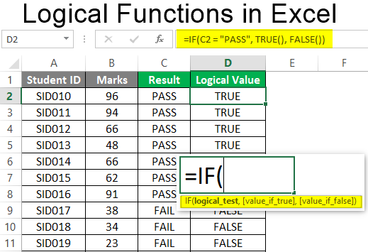
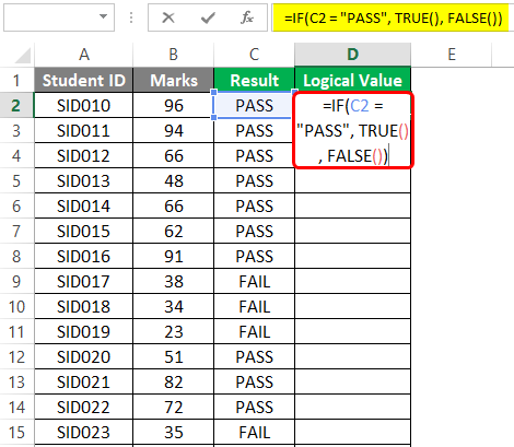
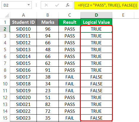
We have the result of students. For PASS, we will display TRUE and for FAIL, FALSE. The following screenshot shows the implementation.
The result that we obtain is as shown below.
Things to Remember
- The logical functions should be implemented in various contexts to understand their full capability.
- The difference in available features in logical functions for different versions of Excel should be checked.
- Each of the argument in a logical function should be studied in order to understand its role and significance.
Recommended Articles
This has been a guide to Logical Functions in Excel. Here we discuss How to use Logical Functions in Excel along with practical examples and a downloadable excel template. You can also go through our other suggested articles –
- Excel Logical Test
- Excel IF AND Function
- AND Function in Excel
- Excel SUMIF with OR
A logical test means having an analytical output that is either TRUE or FALSE. In Excel, we can perform a logical test for any situation. The most commonly used logical test is using the equals to the operator, which is “=” if we use =A1=B1 in cell A2, then it will return TRUE if the values are equal and FALSE if the values are not equal.
What is the Logical Test in Excel?
In Excel, at the beginning stages of learning, it is not easy to understand the concept of logical tests. But once you master this, it will be a valuable skill for your CV. More often than not, in Excel, we use a logical test to match multiple criteriaCriteria based calculations in excel are performed by logical functions. To match single criteria, we can use IF logical condition, having to perform multiple tests, we can use nested IF conditions. But for matching multiple criteria to arrive at a single result is a complex criterion-based calculation.read more and arrive at the desired solution.
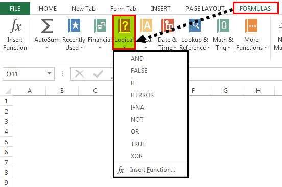
In Excel, we have as many as 9 logical formulas. We must go to the “Formulas” tab and click on the “Logical” function group to see the logical formulas.
Some of them are frequently used formulas, and some of them are rarely used. This article will cover some of the important Excel logical formulas in real-time examples. All the Excel logical formulas work based on TRUE or FALSE if the logical test we do.
Table of contents
- What is the Logical Test in Excel?
- How to Use Logical Function in Excel?
- #1 – AND & OR Logical Function in Excel
- Example #1- AND Logical Function in Excel
- Example #2 – OR Logical Function in Excel
- #2 – IF Logical Function in Excel
- #3 – IF with AND & OR Logical Functions in Excel
- Things to Remember
- Recommended Articles
How to Use Logical Function in Excel?
Below are examples of logical functions in Excel.
You can download this Logical Functions Excel Template here – Logical Functions Excel Template
#1 – AND & OR Logical Function in Excel
Excel AND and OR functions work opposite each other. For example, AND condition in Excel requires all the logical tests to be TRUE. On the other hand, the OR function requires any logical tests to be TRUE.
For example, look at the below examples.
We have student names, marks 1, and marks 2. If the student scored more than 35 in both exams, the result should be TRUE. If not, the result should be FALSE. Since we need to satisfy both the conditions, we need to use AND logical test here.
Example #1- AND Logical Function in Excel
- We must open AND function first.
- The first logical 1 is Marks-1 is >35 or not to test the condition.
- The second test is Marks-2 is >35 or not. So, we must take the logical test.
- We have only two conditions to test. So, we have applied both the logical tests. Now close the bracket.
If both conditions are satisfied, the formula returns TRUE by default. Else, returns FALSE as a result.
Drag the formula to the rest of the cells.
In cells D3 and D4, we got FALSE because in “Marks-1,” both the students scored less than 35.
Example #2 – OR Logical Function in Excel
The Excel OR function is completely different from the AND function. The OR in ExcelThe OR function in Excel is used to test various conditions, allowing you to compare two values or statements in Excel. If at least one of the arguments or conditions evaluates to TRUE, it will return TRUE. Similarly, if all of the arguments or conditions are FALSE, it will return FASLE.read more requires only one condition to be TRUE. Therefore, we must apply the same logical test to the above data with OR conditions.
We will have results in either FALSE or TRUE. Here, we got TRUE.
Drag the formula to other cells.
Now, look at the difference between AND and OR functions. The OR function returns TRUE for students B and C even though they have scored less than 35 in one of the exams. However, since they scored more than 35 in Marks 2, the OR function found the condition of >35 TRUE in 2 logical tests and returned TRUE as a result.
#2 – IF Logical Function in Excel
The IF excel FunctionIF function in Excel evaluates whether a given condition is met and returns a value depending on whether the result is “true” or “false”. It is a conditional function of Excel, which returns the result based on the fulfillment or non-fulfillment of the given criteria.
read more is one of the important logical functions to discuss in Excel. It includes three arguments to supply. Now, look at the syntax.
- Logical Test: It is nothing but our conditional test.
- Value if True: If the above logical test in Excel is TRUE, what should be the result.
- Values if FALSE: If the above logical test in Excel is FALSE, what should be the result.
For example, take a look at the below data.
If the product’s price is more than 80, we need the result as “Costly.” On the other hand, if the product’s price is less than 80, we need the result as “OK.”
Step 1: Here, the logical test is whether the price is >80 or not. So, we must open the IF condition first.
Step 2: Now pass the logical test in Excel, Price >80.
Step 3: If the logical test in Excel is TRUE, we need the result as “Costly.” So in the next argument, VALUE, if TRUE, mentions the result in double-quotes as “Costly.”
Step 4: The final argument is if the logical test in Excel is FALSE. If the test is FALSE, we need the result to be “OK.”
We got the result of “Costly.”
Step 5: Drag the formula to other cells to have the result in all the cells.
Since the orange and sapota price is less than 80, we got the result as “OK.” However, the logical test in Excel is >80, so we got “Costly” for apples and grapes because their price is > 80.
#3 – IF with AND & OR Logical Functions in Excel
The IF function with the other two logical functions (AND & OR) is one of the best combination formulas in Excel. For better understanding, look at the below example data, which we have used for AND and OR conditions.
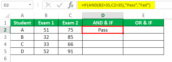
If the student scored more than 35 in both the exams, it would declare him a PASS or FAIL.
The AND function, by default, can only return TRUE or FALSE as a result. But here, we need the results as PASS or FAIL. So, we have to use the IF condition here.
Open the IF condition first.
If we can only test one condition simultaneously, we need to look at two conditions. So, we must open AND condition and pass the tests as Exam 1 >35 and Exam 2>35.
If both the supplied conditions are TRUE, we need the result as “PASS.” So mention the value “PASS” if the logical test in Excel is “TRUE.”
If the logical test in Excel is “FALSE,” the result should be “FAIL.”
So, here we got the result as “PASS.”
Drag the formula to other cells.
So, instead of default TRUE or FALSE, we got our values with the help of the IF condition. Similarly, we can also apply the OR function and replace the OR function with the IF and AND functions.
Things to Remember
- The AND functionThe AND function in Excel is classified as a logical function; it returns TRUE if the specified conditions are met, otherwise it returns FALSE.read more requires all the logical tests in Excel to be TRUE.
- The OR function requires at least any logical tests to be TRUE.
- We have other logical tests in Excel like the IFERROR function in excelThe IFERROR function in Excel checks a formula (or a cell) for errors and returns a specified value in place of the error.read more, NOT function in excelNOT Excel function is a logical function in Excel that is also known as a negation function and it negates the value returned by a function or the value returned by another logical function.read more, TRUE Function in excelIn Excel, the TRUE function is a logical function that is used by other conditional functions such as the IF function. If the condition is met, the output is true; if the conditions are not met, the output is false.read more, FALSE, etc.…
- We will discuss the remaining Excel logical tests in a separate article.
Recommended Articles
This article is a guide to Logical Tests in Excel. We discuss logical functions like AND, OR, and IF in Excel, practical examples, and a downloadable template. You may also learn more about Excel from the following articles: –
- SUMIF with Multiple CriteriaThe SUMIF (SUM+IF) with multiple criteria sums the cell values based on the conditions provided. The criteria are based on dates, numbers, and text. The SUMIF function works with a single criterion, while the SUMIFS function works with multiple criteria in excel.read more
- IFERROR in Excel VBAThe IFERROR function in Excel is used to determine what to do when an error occurs before performing any function.read more
- SUMPRODUCT in Excel with Multiple CriteriaIn Excel, using SUMPRODUCT with several Criteria allows you to compare different arrays using multiple criteria.read more
- VLookup Function with IFIn Excel, vlookup is a reference function, and IF is a conditional statement. Based on the results of the Vlookup function, they locate a value that meets the criteria and also matches the reference value.read more
Logical functions in Excel help make comparisons and arrive at a logical conclusion. Here are the logical functions available in Excel and how to use them with examples.
List of Logical Functions
Let’s go over the list of logical functions that are available in excel and learn how we can use them in our day-to-day work.
1. AND function
AND function is one of the logical functions in Excel, which determines whether all criteria in a test are TRUE. it returns TRUE if all of its parameters are TRUE, and FALSE if one or more arguments are FALSE.
Syntax: AND(logical1, [logical2], …), where logical1 is the first condition you want to test is one that can be TRUE or FALSE and logical2… are optional and additional conditions up to a maximum of 255 conditions.
The following example shows the use of AND function:
- Select the cell where you want to display the result.
- Type =AND(A1>50,B1<50) where cells A1 and B1 contain numeric values.

- Press the Enter key to display the result.

2. FALSE function
The FALSE function in Excel returns the logical FALSE value.
Syntax: FALSE(), it has no arguments. Microsoft Excel will read the word FALSE without parentheses as the logical value FALSE if you write it directly onto the worksheet or into a formula.
3. IF function
One of Excel’s most used tools is the IF function, which allows you to create logical comparisons. An IF statement can have two possible outcomes. If the comparison is TRUE, the first result is returned; if the comparison is FALSE, the second result is returned.
Syntax: IF(logical_test,value_if_true,[value_if_false]), where logical_test is the comparison you want to test, value_if_true is the value to be returned if the logical_test is TRUE, and value_if_false is the value to b returned if the logical_test is FALSE. The following example shows the use of the IF function:
- Select the cell where you want to display the result.
- Type =IF(A1>B1,”A1>B1″,”A1<B1″) where cells A1 and B1 contain numeric values.

- Press the Enter key to display the result.

4. IFERROR function
The IFERROR function can be used to catch and manage errors in a formula. If a formula evaluates to an error, IFERROR returns a value you specify; otherwise, it returns the formula’s result.
Syntax: IFERROR(value, value_if_error), where value is the condition to be checked for #N/A, #VALUE!, #REF!, #DIV/0!, #NUM!, #NAME?, or #NULL! error and value_error is the custom message to be returned if the formula evaluates to an error. The following example shows the use of the IFERROR function:
- Select the cell where you wan to display the result.
- Type =IFERROR(A2/B2,”Error in calculation”) where cells A2 and B2 contain the dividend and divisor respectively.

- Press the Enter key to display the result. As, you can see the divisor is zero, so a #DIV/0! should be returned. IFERROR fucntion catches the error and returns the custom message.

5. IFS function
The IFS function determines whether one or more criteria are met and returns the value corresponding to the first TRUE condition. With several criteria, IFS can replace nested IF statements and is considerably easier to read.
Syntax: IFS(logical_test1, value_if_true1, [logical_test2, value_if_true2], [logical_test3, value_if_true3],…), where logical_test1 is the first comparison you want to test, value_if_true 1 is the value to be returned if the logical_test1 is TRUE and the same follows for other conditions. The following example shows the use of IFS function:
- Select the cell where you want to display the result.
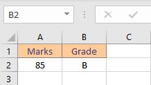
- Type =IFS(A2>89,”A”,A2>79,”B”,A2>69,”C”,A2>59,”D”,A2<=59,”F”) to assign letter grades on the basis of marks obtained.

- Press the Enter key to display the result. The value returned is “B” as 85>79 and 85<90.
6. NOT function
The NOT function returns the inverse of its argument’s value. It is frequently used to extend the utility of other functions that perform logical tests.
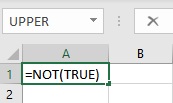
Syntax: NOT(logical), where logical is a value or expression that may be tested to determine whether it is TRUE or FALSE. The following example shows the use of the NOT function:
- Select the cell where you want to display the result.
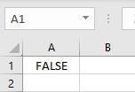
- Type =NOT(TRUE), to reverse TRUE value to FALSE.
- Press the Enter key to display the result.
7. OR function
The OR function returns TRUE if any of its parameters are TRUE and FALSE if all of its arguments are FALSE.
Syntax: OR(logical1, [logical2], …), where logical1, logical2, logical3 etc, are conditions to be evaluated for TRUE and FALSE values. The following example shows the use of the OR function:
- Select the cell where you want to display the result.
- Type =OR(A1<50,B1>50) where cells A1 and B1 contain numeric values.

- Press the Enter key to display the result.

8. SWITCH function
The SWITCH function compares one value called the expression to a list of values and returns the first matched value as the result. If no match is found, a default value is returned.
Syntax: SWITCH(expression, value1, result1, [default or value2, result2],…[default or value3, results]), where expression is the value to be compared, value1… are the values to compare an expression to, and result1… are the results to be returned corresponding to the matching value of the expression. The following example shows the use of the SWITCH function:
- Select the cell where you want to display the result.
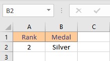
- Type =SWITCH(A2,1,”Gold”,2,”Silver”,3,”Bronze”) to decide medals on the basis of rank in cell A2.

- Press the Enter key to display the result.
9. TRUE function
The TRUE function in Excel returns the logical TRUE value.
Syntax: TRUE(), it has no arguments. Microsoft Excel will read the word TRUE without parentheses as the logical value TRUE if you write it directly onto the worksheet or into a formula.
10. XOR function
The XOR function returns a TRUE value when the number of true inputs is odd otherwise it returns FALSE. Syntax: XOR(logical1, [logical2],…), where logical1, logical2, logical3 etc, are conditions to be evaluated for TRUE or FALSE values. The following example shows the use of XOR function:
- Select the cell where you want to display the result.
- Type =XOR(A1>50,B1<50,C1<25) where cells A1, B1 and C1 contain numeric values.

- Press the Enter key to display the result. The XOR fucntion returns FALSE value as 2 conditions are TRUE and 2 is an even number.

Conclusion
In this article, we learned about the various logical functions in Excel.
References
- AND function (microsoft.com)
- FALSE function (microsoft.com)
- IF function (microsoft.com)
- IFERROR function (microsoft.com)
- IFS function (microsoft.com)
- NOT function (microsoft.com)
- OR function (microsoft.com)
- SWITCH function (microsoft.com)
- TRUE function (microsoft.com)
- XOR function (microsoft.com)


