
-
Select the cell where you want the result to appear.
-
On the Formulas tab, click More Functions, point to Statistical, and then click one of the following functions:
-
COUNTA: To count cells that are not empty
-
COUNT: To count cells that contain numbers.
-
COUNTBLANK: To count cells that are blank.
-
COUNTIF: To count cells that meets a specified criteria.
Tip: To enter more than one criterion, use the COUNTIFS function instead.
-
-
Select the range of cells that you want, and then press RETURN.
-
Select the cell where you want the result to appear.
-
On the Formulas tab, click Insert, point to Statistical, and then click one of the following functions:
-
COUNTA: To count cells that are not empty
-
COUNT: To count cells that contain numbers.
-
COUNTBLANK: To count cells that are blank.
-
COUNTIF: To count cells that meets a specified criteria.
Tip: To enter more than one criterion, use the COUNTIFS function instead.
-
-
Select the range of cells that you want, and then press RETURN.
Excel for Microsoft 365 Excel for Microsoft 365 for Mac Excel for the web Excel 2021 Excel 2021 for Mac Excel 2019 Excel 2019 for Mac Excel 2016 Excel 2016 for Mac Excel 2013 Excel 2010 Excel 2007 Excel for Mac 2011 Excel Starter 2010 More…Less
The COUNT function counts the number of cells that contain numbers, and counts numbers within the list of arguments. Use the COUNT function to get the number of entries in a number field that is in a range or array of numbers. For example, you can enter the following formula to count the numbers in the range A1:A20: =COUNT(A1:A20). In this example, if five of the cells in the range contain numbers, the result is 5.

Syntax
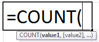
COUNT(value1, [value2], …)
The COUNT function syntax has the following arguments:
-
value1 Required. The first item, cell reference, or range within which you want to count numbers.
-
value2, … Optional. Up to 255 additional items, cell references, or ranges within which you want to count numbers.
Note: The arguments can contain or refer to a variety of different types of data, but only numbers are counted.
Remarks
-
Arguments that are numbers, dates, or a text representation of numbers (for example, a number enclosed in quotation marks, such as «1») are counted.
-
Logical values and text representations of numbers that you type directly into the list of arguments are counted.
-
Arguments that are error values or text that cannot be translated into numbers are not counted.
-
If an argument is an array or reference, only numbers in that array or reference are counted. Empty cells, logical values, text, or error values in the array or reference are not counted.
-
If you want to count logical values, text, or error values, use the COUNTA function.
-
If you want to count only numbers that meet certain criteria, use the COUNTIF function or the COUNTIFS function.
Example
Copy the example data in the following table, and paste it in cell A1 of a new Excel worksheet. For formulas to show results, select them, press F2, and then press Enter. If you need to, you can adjust the column widths to see all the data.
|
Data |
||
|
12/8/08 |
||
|
19 |
||
|
22.24 |
||
|
TRUE |
||
|
#DIV/0! |
||
|
Formula |
Description |
Result |
|
=COUNT(A2:A7) |
Counts the number of cells that contain numbers in cells A2 through A7. |
3 |
|
=COUNT(A5:A7) |
Counts the number of cells that contain numbers in cells A5 through A7. |
2 |
|
=COUNT(A2:A7,2) |
Counts the number of cells that contain numbers in cells A2 through A7, and the value 2 |
4 |
Need more help?
What Is COUNT In Excel?
The COUNT function in Excel counts the number of cells containing numerical values within the given range. It always returns an integer value.
The COUNT in Excel is an inbuilt statistical function, so we can insert the formula from the “Function Library” or enter it directly in the worksheet.
For example, to count a range of cells that contain a date before April 1, 2021, the formula used is “=COUNT(“Cell Range”, “<”&DATE (2021,4,1))”. The date is entered by using the DATE functionThe date function in excel is a date and time function representing the number provided as arguments in a date and time code. The result displayed is in date format, but the arguments are supplied as integers.read more.
Table of contents
- What Is COUNT In Excel?
- Syntax Of COUNT Excel Formula
- How To Use COUNT Function In Excel?
- Examples
- The Characteristics Of The COUNT Function
- Important Things To Note
- Frequently Asked Questions (FAQs)
- COUNT Function In Excel Video
- Download Template
- Recommended Articles
- In a given dataset, the COUNT function in Excel returns the count of the numeric values.
- It counts only the numbers and not the logical values, empty cells, text, or error values when the argument seems to be an array or reference.
- The usage of the COUNT and VBA (VBA Excel COUNT) functions are the same in Excel.
- The COUNTA function is a further extension of the COUNT function. It counts logical values, text, or error values. The COUNTIF function (another extension of the COUNT function) counts the numbers that meet a specified criterion.
Syntax Of COUNT Excel Formula
The syntax of the COUNT Excel formula is,
The arguments of the COUNT Excel formula are,
- value1, [value2], …, [value n]: It is a mandatory argument. It can range up to 255 values. The value can be a cell referenceCell reference in excel is referring the other cells to a cell to use its values or properties. For instance, if we have data in cell A2 and want to use that in cell A1, use =A2 in cell A1, and this will copy the A2 value in A1.read more or a range of values. It is a collection of worksheet cells containing a variety of data, out of which only the cells containing numbers are counted.
How To Use COUNT Function In Excel?
We can use the COUNT Excel function in 2 ways, namely:
- Access from the Excel ribbon.
- Enter in the worksheet manually.
Method #1 – Access from the Excel ribbon
Choose an empty cell for the result → select the “Formulas” tab → go to the “Function Library” group → click the “More Functions” option drop-down → click the “Statistical” option right arrow → select the “COUNT” function, as shown below.

The “Function Arguments” windowappears. Enter the arguments in the “Value1”, “Value2”, etc. fields, and click “OK”, as shown below.

Method #2 – Enter in the worksheet manually
- Select an empty cell for the output.
- Type =COUNT( in the selected cell. [Alternatively, type =C or =COU and double-click the COUNT function from the list of suggestions shown by Excel.
- Enter the argument as cell value or cell reference and close the brackets.
- Press the “Enter” key.
Basic Example – Count Numbers in the Given Range
Let us look at an example to apply the COUNT function to Count Numbers in the Given Range. (shown in the table below).
Select cell B10, enter the formula =COUNT(B3:B8), and press “Enter”.
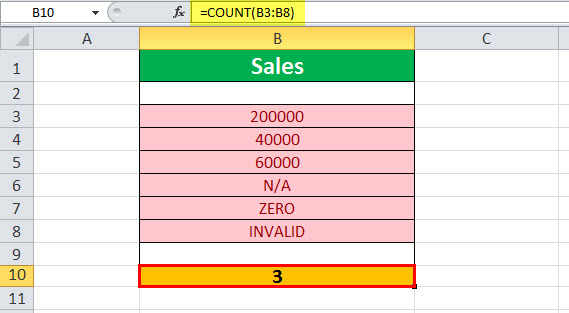
The output is shown above. The range B3:B8 contains only three numeric values. Hence, the COUNT function returns 3.
Examples
We will consider some scenarios using COUNT Function in Excel examples. Each example covers a different case, implemented using the COUNT function.
Example #1 – Count Non-empty Cells
Let us apply the COUNTA functionThe COUNTA function is an inbuilt statistical excel function that counts the number of non-blank cells (not empty) in a cell range or the cell reference. For example, cells A1 and A3 contain values but, cell A2 is empty. The formula “=COUNTA(A1,A2,A3)” returns 2.
read more to the range of cells A1:A5 provided in the below table to find the count of the number of cells that are not empty.
Select cell B1, enter the formula =COUNTA(A1:A5), and press “Enter”.

The output is shown above. The COUNTA function counts the number of cells from A1 through A5 that contain some data. It returns the value as 4, as cells A1, A2, A3, and A4 are not empty, and only cell A5 is empty.
Example #2 – Count the Number of Valid Dates
Let us apply the COUNT function to count the number of valid dates to the range of cells C3:C8 (shown in the table below).
Select cell C10, enter the formula =COUNT(C3:C8), and press “Enter”.
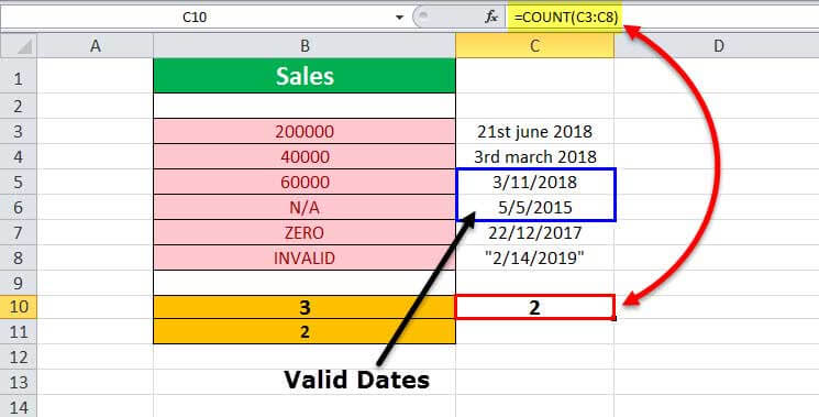
The output is shown above. The range contains dates in different formats. Out of this, only two dates are valid. Hence, the formula returns 2.
Example #3 – Multiple Parameters
Let us apply the COUNT formula to the range of excel cells C3:C7 (provided in the table below) along with another parameter that is hard-coded with a value of 5.
Select cell C11, enter the formula =COUNTA(C3:C7,5), and press “Enter”.
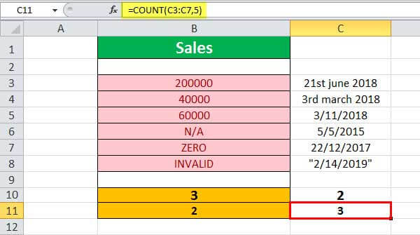
The output is shown above. The number of cells (C3 through C7) with valid numeric values or dates is 2, plus 1 for the number 5. Hence the COUNT formula returns the result as 3 (cells C5, C6, and the number 5). Note that the date in cell C7 is invalid, and so is not taken into account in the given results.
Example #4 – Invalid Numbers
Let us apply the COUNT formula to the range of values B6:B8 (shown in the table below) containing invalid numbers.
Select cell B12, enter the formula =COUNTA(B6:B8), and press “Enter”.
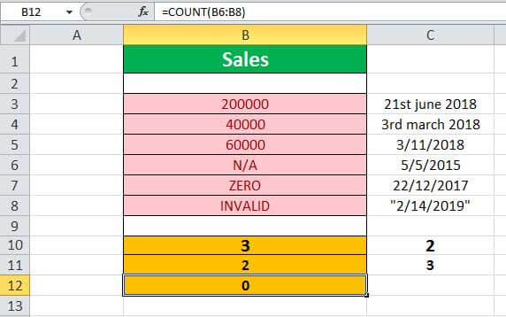
The output is shown above. The range does not have any valid number. Hence, the result returned by the formula is 0, indicated in cell B12.
Example #5 – Empty Range
Let us apply the COUNT function to the range of values in cells D3:D5, which is an empty range.
Select cell D10, enter the formula =COUNTA(D3:D5), and press “Enter”.

The output is shown above. The given range does not have any numbers, and it is empty. Hence, the result returned by the formula is 0, indicated in cell D10.
The Characteristics Of The COUNT Function
The features of the COUNT Excel function are listed as follows:
- It counts the list of parameters containing the logical values and text representations.
- It does not count the error values or text which cannot be converted into numbers.
- It counts only the numbers and not the logical values, empty cells, text, or error values when the argument seems to be an array or reference.
- A further extension to the COUNT function is the COUNTA function. It counts logical values, text, or error values.
- Another extension of the COUNT function is the COUNTIF function, which counts the numbers that meet a specified criterion.
Important Things To Note
- Since the COUNT function has other related functions such as COUNTA, COUNTIF, COUNTBLANK, etc., we must ensure we enter the right function name to avoid getting a “#NAME?” error.
- In a selected cell range, the function ignores the blank cells, non-numeric cells, etc.
Frequently Asked Questions (FAQs)
1. How to use the Excel COUNT function?
The COUNT function provides the count of cells containing numbers within the given range of cells. It also counts numeric values within the list of arguments.
The formula of the COUNT in excel is =COUNT(value 1, [value 2],……, and so on).
2. What is the COUNTIF formula?
The COUNTIF function counts cells in a range that meets a single criterion. It counts cells that contain dates, numbers, and text.
The COUNTIF formula in excel is =COUNTIF(range, condition)
Here, the range is a series of cells to count.
3. What is the difference between the COUNT and COUNTA functions in Excel?
The COUNT function is generally used to count a range of cells containing numbers or dates. It excludes blank cells. And the COUNTA function, whichstands for count all, will count the numbers, dates, text, or a range containing a mixture of all these items. It does not count blank cells.
COUNT Function In Excel Video
Download Template
This article must help understand the COUNT function in Excel with its formulas and examples. You can download the template here to use it instantly.
You can download this COUNT Formula Excel Template here – COUNT Formula Excel Template
Recommended Articles
This is a guide to the COUNT Function in Excel. Here, we count number of cells with numeric values, COUNTA, COUNTIF, examples & a downloadable template. You may also look at the below useful functions in Excel –
- Example of COUNTIF with Multiple Criteria
- INT Function in Excel (Integer)INT or integer function in excel returns the nearest integer of a given number and is used when we have many data sets and each data in a different format.read more
- AVERAGE Function in Excel
MS Excel is a good tool for organizational and accounting things and it can be used at any level. It doesn’t require a lot of experience, because the tool is making everything seem easy. You can use it for your personal need too, with powerful functions such as advanced Vlookup in Excel, find the position of a character in a string, or also count number of occurences of a string in a file.
MS Excel is a good tool for organizational and accounting things and it can be used at any level. It doesn’t require a lot of experience, because the tool is making everything seem easy. You can use it for your personal need too, with powerful functions such as advanced Vlookup in Excel, find the position of a character in a string, or also count number of occurences of a string in a file.
The best part of using the MS Excel is that it has a lot of features and so you can even count the cells and count characters in a cell. Counting the cells manually is no longer a comfortable thing.
How to count number of cells in Excel
First, we will start with counting the cells. Because the MS Excel has a lot of counting features, there’s no need for you to worry if it’s right or wrong.
#1 — Click left on an empty cell, where you want the result to appear. Usually, this happens on the right cell after a row or in the bottom on completed cells.
#2 — The formula tab is right above the cells. Because finding the functions it can be quite challenging, you can simply write =COUNTA on the formula tab. After the word ‘=COUNTA’, you will open some round parenthesis and write the number of the cells from which you want to get a result (e.g C1,C2,C3 etc.).
How to count number of cells: =COUNTA(C1,C2,C3)If you want to count the cells with a specific criteria (e.g. consecutive numbers), you will use the COUNTIF function. It works the same way as the COUNT function, but you have to change what’s between the round parenthesis.
E.g. You are looking for numbers that are identically with the number in the C19 cell. In the formula tab, you will write: (C1:C2, C19).
How to to count number of cells in Excel matching criteria: =COUNTIF(C1:C99,X)Also, there is a COUNTIFS function that works with multiple criteria.
How to count number of celles in Excel matching multiple criteria: =COUNTIFS C1:C2, C19, C24:C32, B21)How to number cells in excel?
There are three easy ways to number rows in Excel in order.
1. The first and easiest way to automatically number rows in an Excel spreadsheet.
You will have to manually enter the first two numbers — and these do not have to be 1 and 2. You can start counting from any number. Select the cells with the LMB and move the cursor over the corner of the selected area. The arrow should change to a black cross.
When the cursor turns into a cross, press the left mouse button again and drag the selection to the area in which you want to number the rows or columns. The selected range will be filled with numeric values in increments, as between the first two numbers.
2. A way to number lines using a formula.
You can also assign a number to each line through a special formula. The first cell must contain the seed. Specify it and move on to the next cell. Now we need a function that will add one (or another necessary numbering step) to each subsequent value. It looks like this:
"=[cell with first value] + 1"In our case, this is =A1+1. To create a formula, you can use the SUM button from the top menu — it will appear when you put the = sign in the cell.
We click on the cross in the corner of the cell with the formula and select the range to fill in the data. The lines are numbered automatically. 3. Row numbering in Excel using progression.
You can also add a marker in the form of a number using the Progression function — this method is suitable for working with large lists if the table is long and contains a lot of data.
- In the first cell — we have it A1 — you need to insert the initial number.
- Next, select the required range, capturing the first cell.
- In the Home tab, you need to find the Fill function.
- Then select Progression. The default parameters are suitable for numbering: type — arithmetic, step = 1.
- Click OK and the selected range will turn into a numbered list.
How to count characters in a cell in Excel
In order to count characters in a single cell in Excel, or to count digits in a cell as well, all you have to do is to use one single function.
Count digits in a cell: =LEN(C1)How to count characters in multiple cells in Excel
Counting characters in several cells from a text it is again very interesting and not that hard as any other people would say. You only need to know and use some functions. At least the counting is made by a machine.
There are two functions that works for a smart character counting — SUMPRODUCT and LEN.
#1 — You choose the number of cells that have the text you want to be counted.
C1, C2, C3, C4 and C5.#2 — In the formula tab you will first write the SUMPRODUCT function and after the LEN function. Always in this order.
Count digits in cells: =SUMPRODUCT(LEN(B1:B5))Keep in mind that there’s no need to press the space bar between the parenthesis and the words you are writing when it comes about functions.
Also, the two dots represents the phrase: from …. to …. . In our case: from B1 to B5.
Of course, there are many other functions but this is the one that works well and is very easy to use.
How to count character occurence in cells
If you want to count a specific character in your text, the functions you will need to use are:
SUMPRODUCT, SUBSTITUTE, LENLet’s say you want to see how many times the letter a in lower case appears in your text. And your text is placed in the cells B2 to B9.
The way you will use the functions will be:
Excel count character occurrences in range: =SUMPRODUCT(LEN(B2:B9)-LEN(SUBSTITUTE(B2:B9,"a","")))Using MS Excel functions to count digits in a cell or count characters
Keep in mind that whenever you use a MS Excel function, the round parenthesis are a must. Without them, the function software will not do its job.
Go further with string functions by using powerful functions such as advanced Vlookup in Excel, find the position of a character in a string, or also count number of occurences of a string in a file.
How to count colored cells in Excel using formula?
In order to count colored cells in Excel using formula, you must have a column containing numbers.
Add below function on this data range, change the cells from C2:C9 to your own cells, and use the filter on color function.
The result will be the amount of colored cells in Excel counted using a formula.
How to count colored cells in Excel using formula: =SUBTOTAL(102,C2:C9)