To count letters in excel - Word и Excel - помощь в работе с программами

Count characters in cells

Excel for Microsoft 365 Excel for the web Excel 2021 Excel 2019 Excel 2016 Excel 2013 More…Less

When you need to count the characters in cells, use the LEN function—which counts letters, numbers, characters, and all spaces. For example, the length of «It’s 98 degrees today, so I’ll go swimming» (excluding the quotes) is 42 characters—31 letters, 2 numbers, 8 spaces, a comma, and 2 apostrophes.

To use the function, enter =LEN(cell) in the formula bar, then press Enter on your keyboard.

Multiple cells: To apply the same formula to multiple cells, enter the formula in the first cell and then drag the fill handle down (or across) the range of cells.

To get the a total count of all the characters in several cells is to use the SUM functions along with LEN. In this example, the LEN function counts the characters in each cell and the SUM function adds the counts:

=SUM((LEN(
cell1
),LEN(
cell2
),(LEN(
cell3
))
)).

Give it a try

Here are some examples that demonstrate how to use the LEN function.

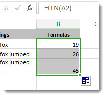
Copy the table below and paste it into cell A1 in an Excel worksheet. Drag the formula from B2 to B4 to see the length of the text in all the cells in column A.

Text Strings	Formulas
The quick brown fox.	=LEN(A2)
The quick brown fox jumped.
The quick brown fox jumped over the lazy dog.

Count characters in one cell

Click cell B2.
Enter =LEN(A2).

The formula counts the characters in cell A2, which totals to 27—which includes all spaces and the period at the end of the sentence.

NOTE: LEN counts any spaces after the last character.

Count
characters in
multiple cells

Click cell B2.
Press Ctrl+C to copy cell B2, then select cells B3 and B4, and then press Ctrl+V to paste its formula into cells B3:B4.

This copies the formula to cells B3 and B4, and the function counts the characters in each cell (20, 27, and 45).

Count a total number of characters

In the sample workbook, click cell B6.
In the cell, enter =SUM(LEN(A2),LEN(A3),LEN(A4)) and press Enter.

This counts the characters in each of the three cells and totals them (92).

Need more help?

Источник

Microsoft Word allows you count text, but what about Excel? If you need a count of your text in Excel, you can get this by using the COUNTIF function and then a combination of other functions depending on your desired result.

How to count text in Excel

If you want to learn how to count text in Excel, you need to use function COUNTIF with the criteria defined using wildcard *, with the formula: =COUNTIF(range;"*"). Range is defined cell range where you want to count the text in Excel and wildcard * is criteria for all text occurrences in the defined range.

Some interesting and very useful examples will be covered in this tutorial with the main focus on the COUNTIF function and different usages of this function in text counting. Limitations of COUNTIF function have been covered in this tutorial with an additional explanation of other functions such as SUMPRODUCT/ISNUMBER/FIND functions combination. After this tutorial, you will be able to count text cells in excel, count specific text cells, case sensitive text cells and text cells with multiple criteria defined – which is a very good base for further creative Excel problem-solving.

Count Text Cells in Excel

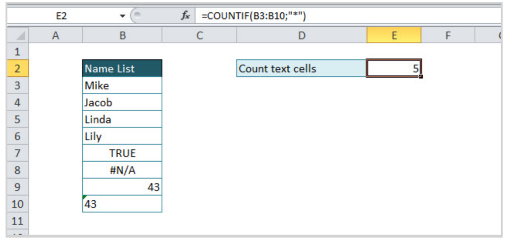
Text Cells can be easily found in Excel using COUNTIF or COUNTIFS functions. The COUNTIF function searches text cells based on specific criteria and in the defined range. As in the example below, the defined range is table Name list, and text criteria is defined using wildcard “*”. The formula result is 5, all text cells have been counted. Note that number formatted as text in cell B10 is also counted, but Booleans (TRUE /FALSE) and error (#N/A) are not recognized as text.

The formula for counting text cells:

=COUNTIF(range;"*")

For counting non-text cells, the formula should be a little bit changed in criteria part:

=COUNTIF(range;"<>*")

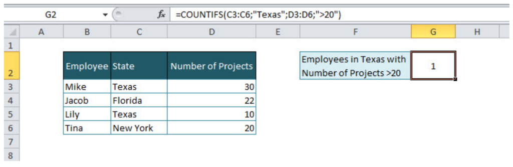
If there are several criteria for counting cells, then COUNTIFS function should be used. For example, if we want to count the number of employees from Texas with project number greater than 20, then the function will look like:

=COUNTIFS(C3:C6;"Texas";D3:D6;">20").

In criteria range in column State, a specific text criteria is defined under quotations “Texas”. The second criteria is numeric, criteria range is column Number of projects, and criteria is numeric value greater than 20, also under quotations “>20”. If we were looking for exact value, the formula would look like:

=COUNTIFS(C3:C6;"Texas";D3:D6;20)

Count Specific Text in Cells

For counting specific text under cells range, COUNTIF function is suitable with the formula:

=COUNTIF(range;"*text*")

=COUNTIF(B3:B9;"*Mike*")

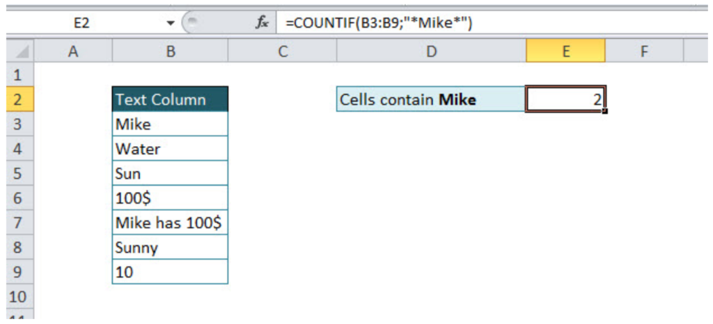
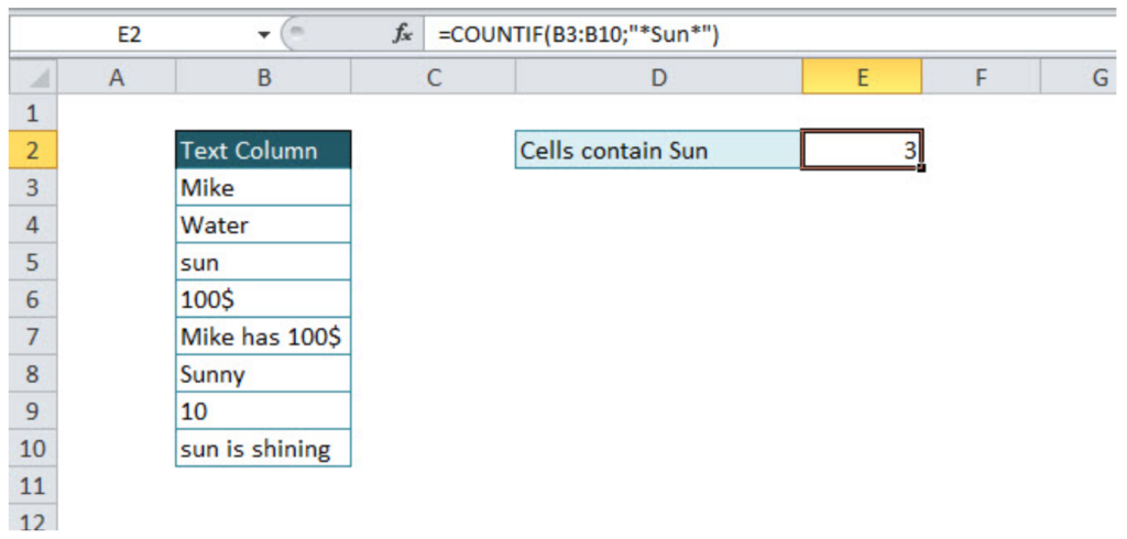
The first part of the formula is range and second is text criteria, in our example “*Mike*”. If wildcard * has not been used before and after criteria text, formula result would have been 1 (Formula would find cells only with word Mike). Wildcard * before and after criteria text, means that all cells that contain criteria characters will be taken into account. As in another example below with text criteria Sun, three cells were found (sun, Sunny, sun is shining)

=COUNTIF(B3:B10;"*Sun*")

Note: The COUNTIF function is not case sensitive, an alternative function for case sensitive text searches is SUMPRODUCT/FIND function combination.

Count Case Sensitive Specific Text

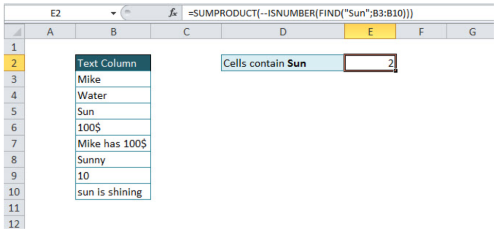
For a case-sensitive text count, a combination of three formulas should be used: SUMPRODUCT, ISNUMBER and FIND. Let’s look in the example below. If we want to count cells that contain text Sun, case sensitive, COUNTIF function would not be the appropriate solution, instead of this function combination of three functions mentioned above has to be used.

=SUMPRODUCT(--ISNUMBER(FIND("Sun";B3:B10)))

We should go through a separate function explanation in order to understand functions combination. FIND function, searches specific text in the defined cell, and returns the number of the starting position of the text used as criteria. This explanation is relevant, if the searching range is just one cell. If we want to use FIND function in a range of the cells, then the combination with SUMPRODUCT function is necessary.

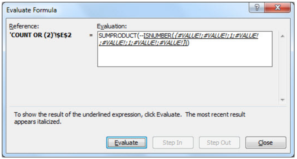
Without ISNUMBER, function combination of FIND and SUMPRODUCT functions would return an error. ISNUMBER function is necessary because whenever FIND function does not match defined criteria, the output will be an error, as in print screen below of the evaluated formula.

In order to change error values with Boolean TRUE/FALSE statement, ISNUMERIC formula should be used (defining numeric values as TRUE, and non-numeric as FALSE, as in print screen below).

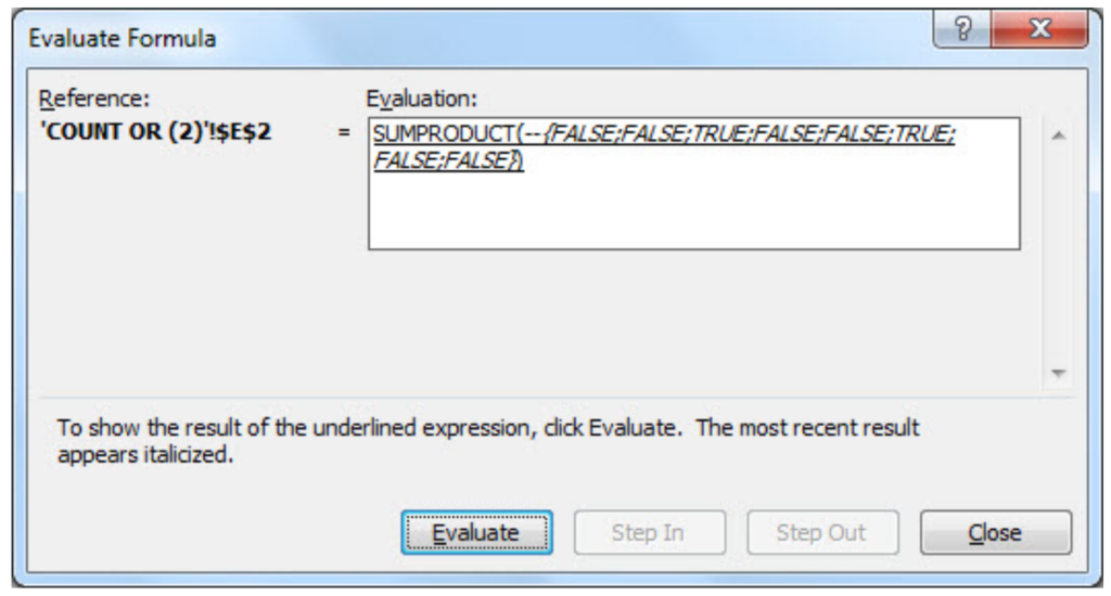
You might be wondering what character — in SUMPRODUCT function stands for. It converts Boolean values TRUE/FALSE in numeric values 1/0, enabling SUMPRODUCT function to deal with numeric operations (without character — in SUMPRODUCT function, the final result would be 0).

Remember, if you want to count specific text cells that are not case sensitive, COUNTIF function is suitable. For all case sensitive searches combination of SUMPRODUCT/ISNUMBER/FIND functions is appropriate.

Count Text Cells with Multiple Criteria

If you want to count cells with Multiple criteria, with all criteria acceptable, there is an interesting way of solving that problem, a combination of SUMPRODUCT/ISNUMBER/FIND functions. Please take a look in the example below. We should count all cells that contain either Mike or $. Tricky part could be the cells that contain both Mike and $.

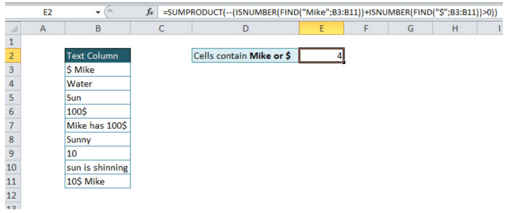
=SUMPRODUCT(--(ISNUMBER(FIND("Mike";B3:B11))+ISNUMBER(FIND("$";B3:B11))>0))

Formula just looks complex, in order to be easier for understanding, I will divide it into several steps. Also, knowledge from the previous tutorial point will be necessary for further work, since the combination of FIND, ISNUMBER, and SUMPRODUCT functions have been explained.

In the first part of the function, we loop through the table and find cells that contain Mike:

=ISNUMBER(FIND("Mike";B3:B11))

The output of this part of the function will be an array with values {1;0;0;0;1;0;0;0;1}, number 1, where criteria have been met, and 0, where has not.

In the second part of the function, looping criteria is $, counting cells containing this value:

=ISNUMBER(FIND("$";B3:B11))

The output of this part of the function will be an array with values {1;0;0;1;1;0;0;0;1}, number 1, where criteria have been met, and 0, where has not.

Next step is to sum these two arrays, since cell should be counted if any of conditions is fulfilled:

=ISNUMBER(FIND("Mike";B3:B11))+ISNUMBER(FIND("$";B3:B11))

The output of this step is {2;0;0;1;2;0;0;0;2}, the number greater than 0 means that one of the condition has been met (2 – both conditions, 1 – one condition)

Without function part >0, the final function would double count cells that met both conditions and the final result would be 7 (sum of all array numbers). In order to avoid it, in the formula should be added >0:

=ISNUMBER(FIND("Mike";B3:B11))+ISNUMBER(FIND("$";B3:B11))>0

The output of this step is array {1;0;0;1;1;0;0;0;1}, the previous array has been checked and only values greater than 0 are TRUE (in an array have value 1), and others are FALSE (in an array have value 0).

Final output of the formula is the sum of the final array values, 4.

Looks very confusing, but after several usages, you will become familiar with this functions.

At the end, we will cover one more multiple criteria text count function, already mentioned in the tutorial, COUNTIFS function. In order to distinguish the usage of functions mentioned above and COUNTIFS function, two words are enough OR/AND. If you want to count text cells with multiple criteria but all conditions have to be met at the same time, then COUNTIFS function is appropriate. If at least one condition should be met, then the combination of function explained above is suitable.

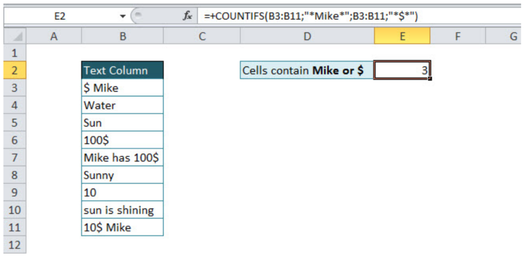
Look at the example below, the number of cells that contain both Mike and $ is easily calculated with COUNTIFS function:

=COUNTIFS(range1;"*text1*";range2;"*text2*")

=COUNTIFS(B3:B11;"*Mike*";B3:B11;"*$*")

In the defined range, function counts only cells where both conditions have been met. The final result is 3.

Still need some help with Excel formatting or have other questions about Excel? Connect with a live Excel expert here for some 1 on 1 help. Your first session is always free.

Источник

Excel has some amazing text functions that can help you when working with the text data.

In some cases, you may need to calculate the total number of characters in a cell/range or the number of times a specific character occurs in a cell.

While there is the LEN function that can count the number of characters in a cell, you can do the rest as well with a combination of formulas (as we will see later in the examples).

In this tutorial, I will cover different examples where you can count total or specific characters in a cell/range in Excel.

Count All Characters in a Cell

If you simply want to get a total count of all the characters in a cell, you can use the LEN function.

The LEN function takes one argument, which could be the text in double-quotes or the cell reference to a cell that has the text.

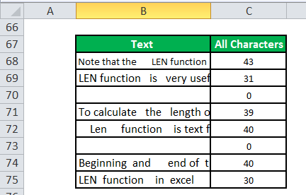
For example, suppose you have the dataset as shown below and you want to count the total number of characters in each cell:

Below is the formula that will do this:

=LEN(A2)

By itself, the LEN function may not look like much, but when you combine it with other formulas, it can do some wonderful things (such as get the word count in a cell or split first and last name).

Note: LEN function will count all the characters in a cell, be it a special character, numbers, punctuation marks, and space characters (leading, trailing, and double spaces between words).

Since the LEN function counts every character in a cell, sometimes you may get the wrong result in case you have extra spaces in the cell.

For example, in the below case, the LEN function returns 25 for the text in cell A1, while it should have been 22. But since it’s counting extra space characters as well, you get the wrong result.

To avoid extra spaces being counted, you can first use the TRIM function to remove any leading, trailing and double spaces and then use the LEN function on it to get the real word count.

Below formula will do this:

=LEN(TRIM(A2))

Count All Characters in a Range of Cells

You can also use the LEN function to count the total number of characters in an entire range.

For example, suppose we have the same dataset and this time, instead of getting the number of characters in each cell, I want to know how many are there in the entire range.

You can do that using the below formula:

=SUMPRODUCT(LEN(A2:A7)))

Let me explain how this formula works.

In the above formula, the LEN part of the function takes an entire range of cells and counts the characters in each cell.

The result of the LEN function would be:

{22;21;23;23;23;31}

Each of these numbers represents the character count in the cell.

And when you use the SUMPRODUCT function with it, it would simply add all these numbers.

Now, if you’re wondering why can’t you use SUM instead of SUMPRODUCT, the reason is that this is an array, and SUMPRODUCT can handle array but the SUM function can not.

However, if you still want to use SUM, you can use the below formula (but remember that you need to use the Control + Shift + Enter to get the result instead of a regular Enter)

=SUM(LEN(A2:A7))

Count Specific Characters in a Cell

As I mentioned that the real utility of the LEN function is when it’ used in combination with other formulas.

And if you want to count specific characters in a cell (it could be a letter, number, special character, or space character), you can do that with a formula combination.

For example, suppose you have the dataset as shown below and you want to count the total number of words in each cell.

While there is no in-built formula to get the word count, you can count the space characters and then use it to know the total number of words in the cell.

Below is the formula that will give you the total number of space characters in a cell:

=LEN(A2)-LEN(SUBSTITUTE(A2," ",""))+1

The above formula counts the total number of space characters and then adds 1 to that number to get the word count.

Here is how this formula works:

SUBSTITUTE function is used to replace all the space characters with a blank. The LEN function is then used to count the total number of characters when there are no space characters.
The result of the LEN(SUBSTITUTE(A2,” “,””)) is then subtracted from LEN(A2). This gives us the total number of space characters that are there in the cell.
1 is added in the formula and the total number of words would be one more than the total number of space characters (as two words are separated with one character).

Note that in case there are any leading, trailing, or double spaces, you are going to get the wrong result. In such a case, it’s best to use the TRIM function along with the LEN function.

You can also use the same logic to find a specific character or word or phrase in a cell.

For example, suppose I have a dataset as shown below where I have different batches, where each batch has an alphabet and number to represent it (such as A1, J2, etc.)

Below is the formula that will give you the total number of times a batch with the alphabet A has been created each month:

=LEN(B2)-LEN(SUBSTITUTE(B2,"A",""))

The above formula again uses the same logic – find the length of the text in a cell with and without the character that you want to count and then take the difference of these two.

In the above formula, I have hardcoded the character that I want to count, but you can also put it in a cell and then use the cell reference. This makes it more convenient as the formula would update the next time you change the text in the cell.

Count Specific Characters Using Case-Insensitive Formula

There is one issue with the formula used to count specific characters in a cell.

The SUBSTITUTE function is case sensitive. This means that you “A” is not equal to “a”. This is why you get the wrong result in cell C5 (the result should have been 3).

So how can you get the character count of a specific character when it could have been in any case (lower or upper).

You do that by making your formula case insensitive. While you can go for a complex formula, I simply added the character count of both the cases (lowercase and uppercase A).

=LEN(B2)-LEN(SUBSTITUTE(B2,"A",""))+LEN(B2)-LEN(SUBSTITUTE(B2,"a",""))

Count Characters/Digits Before and After Decimal

I don’t know why, but this is a common query I get from my readers and have seen in many forums – such as this one

Suppose you have a dataset as shown below and you want to count the characters before the decimal and after the decimal.

Below are the formulas that will do this.

Count characters/numbers before the decimal:

=LEN(INT(A2))

Count characters/numbers after the decimal:

=LEN(A2)-FIND(".",A2)

Note that these formulas are meant only for significant digits in the cell. In case you have leading or trailing zeroes or you have used custom number formatting to show more/fewer numbers, the above formulas would still give you significant digits before and after the decimal.

So these are some of the scenarios where you can use formulas to count characters in a cell or a range of cells in Excel.

I hope you found the tutorial useful!

Other Excel tutorials you may like:

Count Unique Values in Excel Using COUNTIF Function
How to Count Cells that Contain Text Strings
How to Count Colored Cells In Excel
Count Unique Values in Excel Using COUNTIF Function
How To Remove Text Before Or After a Specific Character In Excel

Источник

This post will guide you how to count the number of a given character in a cell in Excel. How do I count only numbers within a single cell excluding all letters and other characters with a formula in Excel. How to count the number of letters excluding all numbers in a given string in Excel.

Count Total Characters in a Cell
Count Only Numbers in a Cell
Count Only Letters or Other Characters Excluding Numbers

Table of Contents

Count Total Characters in a Cell
Count Only Numbers in a Cell
Count Only Letters or Other Characters Excluding Numbers
- Related Functions

Count Total Characters in a Cell

Assuming that you have a list of data in range B1:B4, and you want to count the total number of all characters in one cell, you can use a formula based on the LEN function to get it. Like this:

=LEN(B1)

Type this formula in cell C1 and press Enter key on your keyboard, and drag the AutoFill Handle to copy this formula from Cell C1 to range C2:C4.

count number of letters 1

You should notice that the number of all characters in each cell is calculated.

If you want only count the total numbers in cells, excluding letters and other specific characters, you can use a formula based on the LEN function and the SUBSTITUTE function. Like this:

=LEN(B1)-LEN(SUBSTITUTE(SUBSTITUTE(SUBSTITUTE(SUBSTITUTE(SUBSTITUTE(SUBSTITUTE(SUBSTITUTE(SUBSTITUTE(SUBSTITUTE(SUBSTITUTE(B1,0,""),1,""),2,""),3,""),4,""),5,""),6,""),7,""),8,""),9,""))

Type this formula into a blank cell and press Enter key. And then drag the AutoFill Handle down to other cells to apply this formula.

count number of letters2

Count Only Letters or Other Characters Excluding Numbers

If you want to count only letters and other specific characters in Cells, you can also use another formula based on the LEN function and the SUBSTITUTE function to achieve the result. Like this:

=LEN(SUBSTITUTE(SUBSTITUTE(SUBSTITUTE(SUBSTITUTE(SUBSTITUTE(SUBSTITUTE(SUBSTITUTE(SUBSTITUTE(SUBSTITUTE(SUBSTITUTE(B1,0,""),1,""),2,""),3,""),4,""),5,""),6,""),7,""),8,""),9,""))

Type this formula into a blank cell and press Enter key. And then drag the AutoFill Handle down to other cells to apply this formula.

count number of letters3

Excel Substitute function
The Excel SUBSTITUTE function replaces a new text string for an old text string in a text string.The syntax of the SUBSTITUTE function is as below:= SUBSTITUTE (text, old_text, new_text,[instance_num])….
Excel LEN function
The Excel LEN function returns the length of a text string (the number of characters in a text string).The syntax of the LEN function is as below:= LEN(text)…

Источник

Как быстро сосчитать количество символов в ячейке Excel

В руководстве объясняется, как считать символы в Excel. Вы изучите формулы, позволяющие получить общее количество символов в диапазоне и подсчитывать только определенные символы в одной или нескольких ячейках.

В нашем предыдущем руководстве была представлена функция ДЛСТР , которая позволяет посчитать количество символов в ячейке Excel.

Функция ДЛСТР (LEN в английской версии) полезна сама по себе, а в связи с другими функциями, такими как СУММ, СУММПРОИЗВ и ПОДСТАВИТЬ, она может решать и более сложные задачи. Далее в этом руководстве мы более подробно рассмотрим несколько основных и более сложных выражений для подсчета количества знаков в Excel.

Как посчитать все символы в диапазоне
Как подсчитать определенные знаки в ячейке
Подсчет определенных букв в ячейке без учета регистра
Как посчитать вхождения текста или подстроки в ячейку?
Сколько раз встречается символ в диапазоне?
Подсчет определенных букв в диапазоне без учета регистра.

Как посчитать все символы в диапазоне

Когда дело доходит до подсчета общего количества знаков в нескольких клетках таблицы, сразу приходит на ум решение сделать это для каждой из них, а затем просто сложить эти числа:

=ДЛСТР(A2)+ДЛСТР(A3)+ДЛСТР(A4)

или

=СУММ(ДЛСТР(A2);ДЛСТР(A3);ДЛСТР(A4))

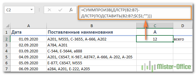
Описанное выше может хорошо работать для небольшого диапазона. Но вряд ли вы захотите таким образом складывать даже 20 чисел. Чтобы определить количество символов Excel в большем диапазоне, нам лучше придумать что-нибудь более компактное. Например, функцию СУММПРОИЗВ, которая перемножает массивы и возвращает сумму произведений.

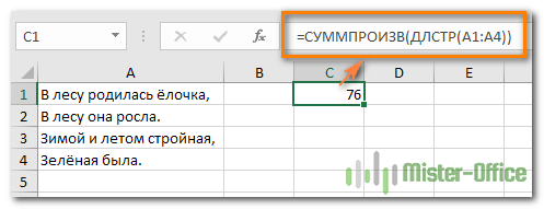
Вот общая формула Эксель для подсчета символов в диапазоне:

=СУММПРОИЗВ(ДЛСТР( диапазон ))

И ваша реальная формула может выглядеть примерно так:

= СУММПРОИЗВ(ДЛСТР(A1:A4))

Другой способ подсчета знаков в диапазоне — использовать функцию ДЛСТР в сочетании с СУММ:

{=СУММ(ДЛСТР(A1:A4))}

В отличие от СУММПРОИЗВ, функция СУММ по умолчанию не вычисляет массивы. Поэтому вам нужно не забыть нажать Ctrl + Shift + Enter, чтобы превратить ее в формулу массива.

Как показано на следующем скриншоте, СУММ возвращает такой же результат:

Как работает эта формула подсчета символов диапазона?

Это один из самых простых вариантов для подсчета знаков в Excel. Перво-наперво функция ДЛСТР вычисляет длину текста для каждого адреса в указанной области и возвращает их в виде массива чисел. Затем СУММПРОИЗВ или СУММ складывают эти числа и возвращают общий итог.

В приведенном выше примере суммируется массив из 4 чисел, которые представляют длины строк в ячейках от A1 до A4:

=СУММПРОИЗВ({23;13;23;17})

Примечание. Обратите внимание, что функция Excel ДЛСТР считает абсолютно все символы в каждой ячейке, включая буквы, числа, знаки препинания, специальные символы и все пробелы (ведущие, конечные и пробелы между словами).

Как подсчитать определенные знаки в ячейке

Иногда вместо подсчета всех символов вам может потребоваться подсчитать только вхождения определенной буквы, числа или специального символа.

Чтобы подсчитать, сколько раз данный символ появляется в выбранной ячейке, используйте функцию ДЛСТР вместе с ПОДСТАВИТЬ:

=ДЛСТР( ячейка ) — ДЛСТР(ПОДСТАВИТЬ( ячейка ; символ ; «»))

Чтобы лучше понять этот расчет, разберём следующий пример.

Предположим, вы ведете базу данных о доставленных товарах, где каждый тип товара имеет свой уникальный идентификатор. И каждая запись содержит несколько элементов, разделенных запятой, пробелом или любым другим разделителем. Задача состоит в том, чтобы подсчитать, сколько раз данный уникальный идентификатор появляется в каждой записи.

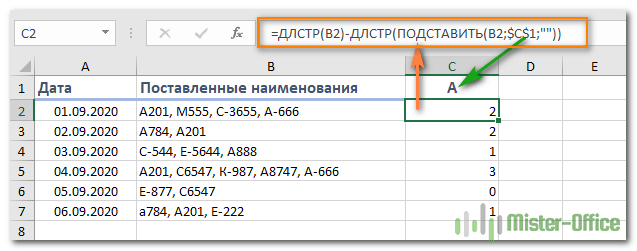
Предполагая, что список доставленных товаров находится в столбце B (начиная с B2), и мы считаем число вхождений «A». Выражение выглядит следующим образом:

=ДЛСТР(B2)-ДЛСТР(ПОДСТАВИТЬ(B2,»A»,»»))

Чтобы понять логику расчётов, давайте разделим процесс на отдельные этапы:

Сначала вы подсчитываете общую длину строки в B2:
ДЛСТР(B2)
Затем вы используете функцию ПОДСТАВИТЬ, чтобы удалить все вхождения буквы «А» в B2, заменив ее пустой строкой («»):
ПОДСТАВИТЬ(B2;»А»;»»)
Затем вы подсчитываете длину получившейся строки без буквы «А»:
ДЛСТР(ПОДСТАВИТЬ(B2;»А»;»»))
Наконец, вы вычитаете длину строки без буквы «А» из первоначальной длины.

В результате вы получаете количество «удаленных» знаков, которое и равно общему числу вхождений этого символа в ячейку.

Вместо того, чтобы указывать букву или цифру, которые вы хотите подсчитать, в формуле, вы можете ввести их, а затем указать на эту ячейку. Таким образом, ваши пользователи смогут подсчитывать вхождения того, что они укажут отдельно, без изменения самой формулы:

Примечание. Функция ПОДСТАВИТЬ в Excel чувствительна к регистру, поэтому в приведенном выше выражении также учитывается регистр. Например, B7 содержит 2 вхождения буквы «A» — одно в верхнем регистре и второе в нижнем регистре. Учитываем только символы верхнего регистра, потому что мы передали «A» функции ПОДСТАВИТЬ.

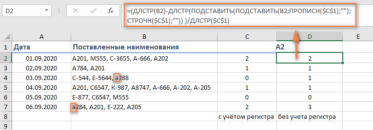
Подсчет определенных букв в ячейке без учета регистра

Если вам нужен счетчик букв без учета регистра, вставьте функцию ПРОПИСН в ПОДСТАВИТЬ, чтобы преобразовать указанную букву в верхний регистр перед выполнением подстановки. И обязательно используйте для поиска заглавные буквы.

Например, чтобы подсчитать буквы «A» и «a» в B2, используйте следующее:

=ДЛСТР(B2)-ДЛСТР(ПОДСТАВИТЬ(ПРОПИСН(B2);$C$1;»»))

Другой способ — использовать вложенные функции замены:

=ДЛСТР(B2)-ДЛСТР(ПОДСТАВИТЬ(ПОДСТАВИТЬ(B2;ПРОПИСН($C$1);»»);СТРОЧН($C$1);»»))

Как вы можете видеть на скриншоте ниже, оба варианта безупречно подсчитывают вхождения указанной буквы в верхнем и нижнем регистре:

Другой способ — преобразовать всё в верхний или нижний регистр. Например:

=ДЛСТР(B2)-ДЛСТР(ПОДСТАВИТЬ(ПРОПИСН(B2);ПРОПИСН($C$1);»»))

Преимущество этого подхода заключается в том, что независимо от того, используются прописные либо строчные буквы, ваша формула подсчета без учета регистра будет возвращать правильный счет:

Как посчитать вхождения текста или подстроки в ячейку?

Если вы хотите подсчитать, сколько раз определенная комбинация символов (например, определенный текст или подстрока) появляется в данной ячейке (например «A2» или «М5»), разделите количество определенных символов, возвращаемых приведенными выше формулами, на длину подстроки.

С учетом регистра:

=(ДЛСТР(B2)-ДЛСТР(ПОДСТАВИТЬ(B2;$C$1;»»)))/ДЛСТР($C$1)

Без учета регистра:

=(ДЛСТР(B2)-ДЛСТР(ПОДСТАВИТЬ(ПОДСТАВИТЬ(B2;ПРОПИСН($C$1);»»);СТРОЧН($C$1);»»)) )/ДЛСТР($C$1)

Где B2 — запись, содержащая всю текстовую строку, а C1 – тот текст (подстроку), который вы хотите подсчитать.

Как эта формула подсчитывает количество вхождений определенного текста в ячейку?

Функция ПОДСТАВИТЬ удаляет указанное слово из исходного текста.
В этом примере мы удаляем слово, введенное в ячейку С1, из исходного текста, расположенного в B2:
ПОДСТАВИТЬ(B2; $C$1;»»)
Затем функция ДЛСТР вычисляет длину текстовой строки без указанного слова.
В этом примере ДЛСТР(ПОДСТАВИТЬ(B2; $C$1;»»)) возвращает длину текста в B2 после удаления всех букв и цифр, содержащихся во всех вхождениях «А2».
После этого указанное выше число вычитается из общей длины исходной текстовой строки:
ДЛСТР(B2)-ДЛСТР(ПОДСТАВИТЬ(B2; $C$1;»»))

Результатом этой операции является количество символов, содержащихся во всех вхождениях целевого слова, которое в этом примере равно 4 (2 вхождения «A2», по 2 в каждом).

Наконец, указанное выше число делится на длину искомого текста. Другими словами, вы делите количество символов, содержащихся во всех вхождениях целевого слова, на число знаков, содержащихся в этом слове. В этом примере 4 делится на 2, и в результате мы получаем 2.

Сколько раз встречается символ в диапазоне?

Теперь, когда вы знаете формулу Excel для подсчета символов в одной определённой ячейке, вы можете улучшить ее, чтобы узнать, сколько раз определенный символ появляется в диапазоне. Для этого мы возьмем выражение, описанное в предыдущем примере, и поместим его в функцию СУММПРОИЗВ, которая умеет обрабатывать массивы:

СУММПРОИЗВ(ДЛСТР( диапазон ) -ДЛСТР(ПОДСТАВИТЬ( диапазон , символ , «»)))

В этом примере выражение принимает следующую форму:

=СУММПРОИЗВ(ДЛСТР(B2:B7)-ДЛСТР(ПОДСТАВИТЬ(B2:B7;$C$1;»»)))

А вот еще один способ для подсчета символов в диапазоне Excel:

{=СУММ(ДЛСТР(B2:B7)-ДЛСТР(ПОДСТАВИТЬ(B2:B7;$C$1;»»)))}

По сравнению с описанным ранее наиболее очевидным отличием здесь является использование СУММ вместо СУММПРОИЗВ. Другое отличие в том, что в данном случае требуется нажатие Ctrl + Shift + Enter. Думаю, вы помните, что в отличие от СУММПРОИЗВ, которая умеет работать с массивами, СУММ может обрабатывать массивы только при использовании её в формуле массива.

Разберем, как это работает.

Как вы, возможно, помните, функция ПОДСТАВИТЬ используется для замены всех вхождений указанного символа («A» в этом примере) пустой текстовой строкой («»).

Затем мы передаем текстовую строку, возвращаемую функцией ПОДСТАВИТЬ, в функцию ДЛСТР, чтобы она вычисляла длину строки без «A». Затем мы вычитаем это количество знаков из общей длины текстовой строки. Результатом этих вычислений является массив количества символов. В нем столько чисел, сколько ячеек в диапазоне.

Наконец, СУММПРОИЗВ суммирует числа в массиве и возвращает общее количество указанного символа в диапазоне.

Примечание. В ситуациях, когда вы подсчитываете количество вхождений определенной подстроки в диапазоне (например, заказы, начинающиеся с «A2»), вам необходимо разделить количество символов на длину подстроки. В противном случае каждый знак в подстроке будет учитываться индивидуально. Например:

=СУММПРОИЗВ(ДЛСТР(B2:B7)-ДЛСТР(ПОДСТАВИТЬ(B2:B7;$C$1;»»)))/ДЛСТР($C$1)

Подсчет определенных букв в диапазоне без учета регистра.

Вы уже знаете, что ПОДСТАВИТЬ — функция, чувствительная к регистру. Поэтому наша формула для подсчета также чувствительна к регистру.

Чтобы игнорировать регистр, следуйте подходам, продемонстрированным в предыдущем примере.

Используйте функции ПРОПИСН и СТРОЧН, введите прописную либо заглавную букву и укажите ссылку на нее:

=СУММПРОИЗВ(ДЛСТР(B2:B7) — ДЛСТР(ПОДСТАВИТЬ(ПОДСТАВИТЬ(B2:B7;ПРОПИСН($C$1);»»);СТРОЧН($C$1);»»)))

На скриншоте ниже показана последняя формула в действии:

Совершенно аналогично, подобный метод можно применить, если мы будем считать число вхождений в диапазон какого- то слова. Вернемся к нашему примеру.

Чтобы подсчитать, сколько раз сочетание «А2» в точном виде встречается в наших данных, запишем выражение:

=СУММПРОИЗВ((ДЛСТР(B2:B7)-ДЛСТР(ПОДСТАВИТЬ(B2:B7;$C$1;»»)))/ДЛСТР($C$1))

Если не нужно учитывать регистр букв, то тогда —

=СУММПРОИЗВ((ДЛСТР(B2:B7)-ДЛСТР(ПОДСТАВИТЬ(ПОДСТАВИТЬ(B2:B7;ПРОПИСН($C$1);»»);СТРОЧН($C$1);»»)))/ДЛСТР($C$1))

То есть, мы берем формулы, использованные нами для отдельной ячейки, меняем в них ссылку на диапазон данных и обрабатываем затем при помощи СУММПРОИЗВ.

Вы можете использовать функцию СУММ, но в формуле массива, как мы также уже рассматривали ранее.

Вот как вы можете подсчитывать символы в Excel с помощью функции ДЛСТР. Если вы хотите знать, как считать слова, а не отдельные знаки, вы найдете несколько полезных формул в нашей следующей статье, следите за обновлениями!

Возможно, вам будут также полезны:

Формула ЗАМЕНИТЬ и ПОДСТАВИТЬ для текста и чисел — В статье объясняется на примерах как работают функции Excel ЗАМЕНИТЬ (REPLACE в английской версии) и ПОДСТАВИТЬ (SUBSTITUTE по-английски). Мы покажем, как использовать функцию ЗАМЕНИТЬ с текстом, числами и датами, а также…

Как быстро посчитать количество слов в Excel — В статье объясняется, как подсчитывать слова в Excel с помощью функции ДЛСТР в сочетании с другими функциями Excel, а также приводятся формулы для подсчета общего количества или конкретных слов в…

Как быстро извлечь число из текста в Excel — В этом кратком руководстве показано, как можно быстро извлекать число из различных текстовых выражений в Excel с помощью формул или специального инструмента «Извлечь». Проблема выделения числа из текста возникает достаточно…

Как убрать пробелы в числах в Excel — Представляем 4 быстрых способа удалить лишние пробелы между цифрами в ячейках Excel. Вы можете использовать формулы, инструмент «Найти и заменить» или попробовать изменить формат ячейки. Когда вы вставляете данные из…

Как удалить пробелы в ячейках Excel — Вы узнаете, как с помощью формул удалять начальные и конечные пробелы в ячейке, лишние интервалы между словами, избавляться от неразрывных пробелов и непечатаемых символов. В чем самая большая проблема с…

Функция СЖПРОБЕЛЫ — как пользоваться и примеры — Вы узнаете несколько быстрых и простых способов, чтобы удалить начальные, конечные и лишние пробелы между словами, а также почему функция Excel СЖПРОБЕЛЫ (TRIM в английской версии) не работает и как…

Функция ПРАВСИМВ в Excel — примеры и советы. — В последних нескольких статьях мы обсуждали различные текстовые функции. Сегодня наше внимание сосредоточено на ПРАВСИМВ (RIGHT в английской версии), которая предназначена для возврата указанного количества символов из крайней правой части…

Функция ЛЕВСИМВ в Excel. Примеры использования и советы. — В руководстве показано, как использовать функцию ЛЕВСИМВ (LEFT) в Excel, чтобы получить подстроку из начала текстовой строки, извлечь текст перед определенным символом, заставить формулу возвращать число и многое другое. Среди…

Источник

The LEN function in Excel is also known as the LENGTH Excel function, which identifies the length of a given string. In addition, this function calculates the number of characters in a given string provided as an input. Therefore, it is a TEXT function in Excel. It is also an inbuilt function that can be accessed by typing =LEN( and providing a string as input.

For example, suppose we type the text “Good Night” in cell A1, and we need to know its characters. Then, we can use the LEN Excel function. In such cases, we can use the following function: LEN(A1), which would return the result 10.

The LEN function is a text function in Excel that returns a string/ text length.

The LEN function in Excel can count the number of characters in a text string and count letters, numbers, special characters, non-printable characters, and all spaces from an Excel cell. In simple words, the LENGTH function is used to calculate the length of a text in an Excel cell.

LEN in Excel
- LEN Formula in Excel
- How to Use LENGTH Function in Excel?
  - LENGTH function in Excel as a worksheet function.
  - Example #1
  - Example #2
  - Example #3
  - Example #4
  - LEN function can be used as a VBA function.
- Things to Remember
- Recommended Articles

LEN Formula in Excel

The LEN formula in Excel has only one critical parameter, text.

Compulsory Parameter:

text: it is the text for which to calculate the length.

How to Use LENGTH Function in Excel?

The LENGTH function in Excel is very simple and easy to use. Let us understand the working of the LENGTH function in Excel by some examples. The LEN function Excel can be used as a worksheet function and a VBA function.

You can download this LEN Function Excel Template here – LEN Function Excel Template

LENGTH function in Excel as a worksheet function.

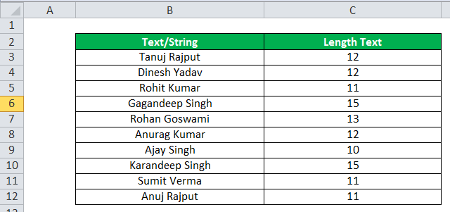
Example #1

In this LEN example, we calculate the length of the given string or text in column 1 and apply the LEN function in column 2. As a result, it will calculate the length of the names provided in column 1, as shown below.

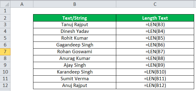
Result:

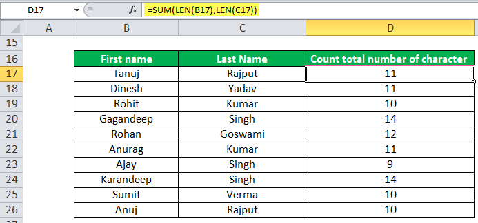
Example #2

We can use the LENGTH function in Excel to calculate the total number of characters in different cells. In this LEN example, we have used the LEN formula in Excel with sum as=SUM(LEN(B17), LEN(C17)) to calculate the total number of characters in different columns, or we can also use =LEN(B17)+LEN(C17) to achieve this.

Result:

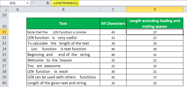
Example #3

We can use the LEN function Excel to count characters in excelTo count characters in excel, use the internal formula called “LEN.” This function counts the letters, numbers, characters, and all spaces present in the cell. Since this function counts everything in the cells, this becomes important to know how to exclude some of the alphabets or values.read more, excluding leading and trailing spaces. We use the length formula in Excel with TRIM to exclude the leading and trailing spaces.

=LEN(TRIM(B31)) and output will be 37.

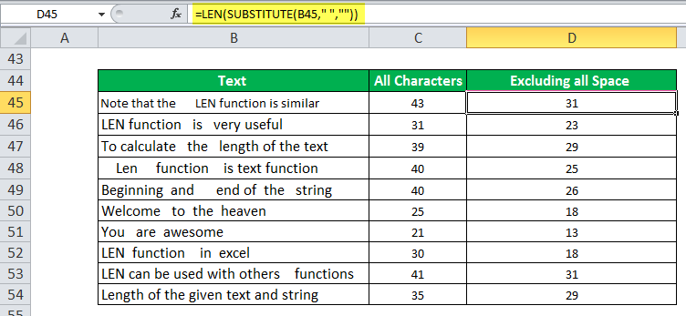
Example #4

We can use the LEN function to count the number of characters in a cell, excluding all spaces. We can use the substitute and LEN formula combination to accomplish this.

=LEN(SUBSTITUTE(B45,” “,””))

LEN function can be used as a VBA function.

Dim LENcount As Long

LENcount = Application.Worksheetfunction.LEN(“Alphabet”)

Msgbox(LENcount) // Return the substring “ab” from string “Alphabet” in the message box.

The output will be “8” and printed in the message box.

Things to Remember

The LENGTH function counts how many characters there are in some string.
We can use it on dates and numbers.

The LEN function does not include formatting length. So, for example, the length of “100” formatted as “$100.00” is still 3).

If the cell is empty, the LENGTH function returns 0 as output.
- As shown in rows three and six, the empty string has 0 lengths.

1. Get Word Count by Excel Formula

=LEN(A1)-LEN(SUBSTITUTE(A1,” “,””))+1

Where:
A1: Cell Address, Where your String is there.

Note:

Here in this Formula, the limitation is that if there are more than One spaces between two words then the Spaces will also be counted as a Word and the Count will not be proper.

2. Get Word Count by User Defined Function (UDF) Macro

Put the below code in Regular Module of your Workbook.

Function GetWordCount(Cell As Range)
    GetWordCount = UBound(Split(Cell.Value, " ")) + 1
End Function

Now you can use the below Formula to get the Word Count
=GetWordCount(Cell Address)

3. Get Letter Count in Excel Formula

=LEN(A1)
Where:
A1: Cell Address, Where your String is there.

Note:

This will return the total count of letters in that cell, including spaces as well.

Источник

Give it a try

Need more help?

How to count text in Excel

Count Text Cells in Excel

Count Specific Text in Cells

Count Case Sensitive Specific Text

Count Text Cells with Multiple Criteria

Count All Characters in a Cell

Count All Characters in a Range of Cells

Count Specific Characters in a Cell

Count Specific Characters Using Case-Insensitive Formula

Count Characters/Digits Before and After Decimal

Count Total Characters in a Cell

Count Only Letters or Other Characters Excluding Numbers

Как посчитать все символы в диапазоне

Как подсчитать определенные знаки в ячейке

Подсчет определенных букв в ячейке без учета регистра

Как посчитать вхождения текста или подстроки в ячейку?

Сколько раз встречается символ в диапазоне?

Подсчет определенных букв в диапазоне без учета регистра.

Table of contents

LEN Formula in Excel

How to Use LENGTH Function in Excel?

LENGTH function in Excel as a worksheet function.

Example #1

Example #2

Example #3

Example #4

LEN function can be used as a VBA function.

Things to Remember

Recommended Articles

1. Get Word Count by Excel Formula

Note:

2. Get Word Count by User Defined Function (UDF) Macro

3. Get Letter Count in Excel Formula

Note: