
Уважаемые коллеги, мы рады предложить вам, разрабатываемый нами учебный курс по программированию ПЛК фирмы Beckhoff с применением среды автоматизации TwinCAT. Курс предназначен исключительно для самостоятельного изучения в ознакомительных целях. Перед любым применением изложенного материала в коммерческих целях просим связаться с нами. Текст из предложенных вам статей скопированный и размещенный в других источниках, должен содержать ссылку на наш сайт heaviside.ru. Вы можете связаться с нами по любым вопросам, в том числе создания для вас систем мониторинга и АСУ ТП.
Типы данных в языках стандарта МЭК 61131-3
Уважаемые коллеги, в этой статье мы будем рассматривать важнейшую для написания программ тему — типы данных. Чтобы читатели понимали, в чем отличие одних типов данных от других и зачем они вообще нужны, мы подробно разберем, каким образом данные представлены в процессоре. В следующем занятии будет большая практическая работа, выполняя которую, можно будет потренироваться объявлять переменные и на практике познакомится с особенностями выполнения математических операций с различными типами данных.
Простые типы данных
В прошлой статье мы научились записывать цифры в двоичной системе счисления. Именно такую систему счисления используют все компьютеры, микропроцессоры и прочая вычислительная техника. Теперь мы будем изучать типы данных.
Любая переменная, которую вы используете в своем коде, будь то показания датчиков, состояние выхода или выхода, состояние катушки или просто любая промежуточная величина, при выполнении программы будет хранится в оперативной памяти. Чтобы под каждую используемую переменную на этапе компиляции проекта была выделена оперативная память, мы объявляем переменные при написании программы. Компиляция, это перевод исходного кода, написанного программистом, в команды на языке ассемблера понятные процессору. Причем в зависимости от вида применяемого процессора один и тот же исходный код может транслироваться в разные ассемблерные команды (вспомним что ПЛК Beckhoff, как и персональные компьютеры работают на процессорах семейства x86).
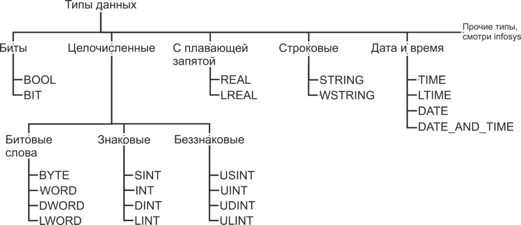
Как помните, из статьи Знакомство с языком LD, при объявлении переменной необходимо указать, к какому типу данных будет принадлежать переменная. Как вы уже можете понять, число B016 будет занимать гораздо меньший объем памяти чем число 4 C4E5 01E7 7A9016. Также одни и те же операции с разными типами данных будут транслироваться в разные ассемблерные команды. В TwinCAT используются следующие типы данных:
Биты
BOOL — это простейший тип данных, как уже было сказано, этот тип данных может принимать только два значения 0 и 1. Так же в TwinCAT, как и в большинстве языков программирования, эти значения, наравне с 0 и 1, обозначаются как TRUE и FALSE и несут в себе количество информации, соответствующее одному биту. Минимальным объемом данных, который читается из памяти за один раз, является байт, то есть восемь бит. Поэтому, для оптимизации скорости доступа к данным, переменная типа BOOL занимает восемь бит памяти. Для хранения самой переменной используется нулевой бит, а биты с первого по седьмой заполнены нулями. Впрочем, на практике о таком нюансе приходится вспоминать достаточно редко.
BIT — то же самое, что и BOOL, но в памяти занимает 1 бит. Как можно догадаться, операции с этим типом данных медленнее чем с типом BOOL, но он занимает меньше места в памяти. Тип данных BIT отсутствует в стандарте МЭК 61131-3 и поддерживается исключительно в TwinCAT, поэтому стоит отдавать предпочтение типу BOOL, когда у вас нет явных поводов использовать тип BIT.
Целочисленные типы данных
BYTE — тип данных, по размеру соответствующий одному байту. Хоть с типом BYTE можно производить математические операции, но в первую очередь он предназначен для хранения набора из 8 бит. Иногда в таком виде удобнее, чем побитно, передавать данные по цифровым интерфейсам, работать с входами выходами и так далее. С такими вопросами мы будем знакомится далее по мере изучения курса. В переменную типа BYTE можно записать числа из диапазона 0..255 (0..28-1).
WORD — то же самое, что и BYTE, но размером 16 бит. В переменную типа WORD можно записать числа из диапазона 0..65 535 (0..216-1). Тип данных WORD переводится с английского как «слово». Давным-давно термином машинное слово называли группу бит, обрабатываемых вычислительной машиной за один раз. Была уместна фраза «Программа состоит из машинных слов.». Со временем этим термином перестали пользоваться в прямом его значении, и сейчас под термином «машинное слово» обычно подразумевается группа из 16 бит.
DWORD — то же самое, что и BYTE, но размером 32 бит. В переменную типа DWORD можно записать числа из диапазона 0..4 294 967 295 (0..232-1). DWORD — это сокращение от double word, что переводится как двойное слово. Довольно часто буква «D» перед каким-либо типом данных значит, что этот тип данных в два раза длиннее, чем исходный.
LWORD — то же самое, что и BYTE, но размером 64 ;бит. В переменную типа LWORD можно записать числа из диапазона 0..18 446 744 073 709 551 615 (0..264-1). LWORD — это сокращение от long word, что переводится как длинное слово. Приставка «L» перед типом данных, как правило, означает что такой тип имеет длину 64 бита.
SINT — знаковый тип данных, длинной 8 бит. В переменную типа SINT можно записать числа из диапазона -128..127 (-27..27-1). В отличии от всех предыдущих типов данных этот тип данных предназначен для хранения именно чисел, а не набора бит. Слово знаковый в описании типа означает, что такой тип данных может хранить как положительные, так и отрицательные значения. Для хранения знака числа предназначен старший, в данном случае седьмой, разряд числа. Если старший разряд имеет значение 0, то число интерпретируется как положительное, если 1, то число интерпретируется как отрицательное. Приставка «S» означает short, что переводится с английского как короткий. Как вы догадались, SINT короткий вариант типа INT.
USINT — беззнаковый тип данных, длинной 8 бит. В переменную типа USINT можно записать числа из диапазона 0..255 (0..28-1). Приставка «U» означает unsigned, переводится как беззнаковый.
Остальные целочисленные типы аналогичны уже описанным и отличаются только размером. Сведем все целочисленные типы в таблицу.
| Тип данных | Нижний предел | Верхний предел | Занимаемая память |
| BYTE | 0 | 255 | 8 бит |
| WORD | 0 | 65 535 | 16 бит |
| DWORD | 0 | 4 294 967 295 | 32 бит |
| LWORD | 0 | 264-1 | 64 бит |
| SINT | -128 | 127 | 8 бит |
| USINT | 0 | 255 | 8 бит |
| INT | -32 768 | 32 767 | 16 бит |
| UINT | 0 | 65 535 | 16 бит |
| DINT | -2 147 483 648 | 2 147 483 647 | 32 бит |
| UDINT | 0 | 4 294 967 295 | 32 бит |
| LINT | -263 | -263-1 | 64 бит |
| ULINT | 0 | -264-1 | 64 бит |
Выше мы рассматривали целочисленные типы данных, то есть такие типы данных, в которых отсутствует запятая. При совершении математических операций с целочисленными типами данных есть некоторые особенности:
- Округление при делении: округление всегда выполняется вниз. То есть дробная часть просто отбрасывается. Если делимое меньше делителя, то частное всегда будет равно нулю, например, 10/11 = 0.
- Переполнение: если к целочисленной переменной, например, SINT, имеющей значение 255, прибавить 1, переменная переполнится и примет значение 0. Если прибавить 2, переменная примет значение 1 и так далее. При операции 0 — 1 результатом будет 255. Это свойство очень схоже с устройством стрелочных часов. Если сейчас 2 часа, то 5 часов назад было 9 часов. Только шкала часов имеет пределы не 1..12, а 0..255. Иногда такое свойство может использоваться при написании программ, но как правило не стоит допускать переполнения переменных.
Подробно такие нюансы разбираются в пособиях по дискретной математике. Мы на них пока что останавливаться не будем, но о приведенных двух особенностях не стоит забывать при написании программ.
Можно встретить упоминания о данных с фиксированной запятой, это такие данные, в которых количество знаков после запятой строго фиксировано. В TwinCAT типы данных с фиксированной запятой отсутствуют в чистом виде. TwinCAT поддерживает типы данных с плавающей запятой, то есть количество знаков до и после запятой может быть любым в пределах поддерживаемого диапазона.
Типы данных с плавающей запятой
REAL — тип данных с плавающей запятой длинной 32 бита. В переменную типа REAL можно записать числа из диапазона -3.402 82*1038..3.402 82*1038.
LREAL — тип данных с плавающей запятой длинной 64 бита. В переменную типа LREAL можно записать числа из диапазона -1.797 693 134 862 315 8*10308..1.797 693 134 862 315 8*10308.
При присваивании значения типам REAL и LREAL присваиваемое значение должно содержать целую часть, разделительную точку и дробную часть, например, 7.4 или 560.0.
Так же при записи значения типа REAL и LREAL использовать экспоненциальную (научную) форму. Примером экспоненциальной формы записи будет Me+P, в этом примере
- M называется мантиссой.
- e называется экспонентой (от англ. «exponent»), означающая «·10^» («…умножить на десять в степени…»),
- P называется порядком.
Примерами такой формы записи будет:
- 1.64e+3 расшифровывается как 1.64e+3 = 1.64*103 = 1640.
- 9.764e+5 расшифровывается как 9.764e+5 = 9.764*105 = 976400.
- 0.3694e+2 расшифровывается как 0.3694e+2 = 0.3694*102 = 36.94.
Еще один способ записи присваиваемого значения переменной типа REAL и LREAL, это добавить к числу префикс REAL#, например, REAL#7.4 или REAL#560. В таком случае можно не указывать дробную часть.
Старший, 31-й бит переменной типа REAL представляет собой знак. Следующие восемь бит, с 30-го по 23-й отведены под экспоненту. Оставшиеся 23 бита, с 22-го по 0-й используются для записи мантиссы.
В переменной типа LREAL старший, 63-й бит также используется для записи знака. В следующие 11 бит, с 62 по 52-й, записана экспонента. Оставшиеся 52 бита, с 51-го по 0-й, используются для записи мантиссы.
При записи числа с большим количеством значащих цифр в переменные типа REAL и LREAL производится округление. Необходимо не забывать об этом в расчетах, к которым предъявляются строгие требования по точности. Еще одна особенность, вытекающая из прошлой, если вы хотите сравнить два числа типа REAL или LREAL, прямое сравнение мало применимо, так как если в результате округления числа отличаются хоть на малую долю результат сравнения будет FALSE. Чтобы выполнить сравнение более корректно, можно вычесть одно число из другого, а потом оценить больше или меньше модуль получившегося результата вычитания, чем наибольшая допустимая разность. Поведение системы при переполнении переменных с плавающей запятой не определенно стандартом МЭК 61131-3, допускать его не стоит.
Строковые типы данных
STRING — тип данных для хранения символов. Каждый символ в переменной типа STRING хранится в 1 байте, в кодировке Windows-1252, это значит, что переменные такого типа поддерживают только латинские символы. При объявлении переменной количество символов в переменной указывается в круглых или квадратных скобках. Если размер не указан, при объявлении по умолчанию он равен 80 символам. Для данных типа STRING количество содержащихся в переменной символов не ограниченно, но функции для обработки строк могут принять до 255 символов.
Объем памяти, необходимый для переменной STRING, всегда составляет 1 байт на символ +1 дополнительный байт, например, переменная объявленная как «STRING [80]» будет занимать 81 байт. Для присвоения константного значения переменной типа STRING присваемый текст необходимо заключить в одинарные кавычки.
Пример объявления строки на 35 символов:
sVar : STRING(35) := 'This is a String'; (*Пример объявления переменной типа STRING*)
WSTRING — этот тип данных схож с типом STRING, но использует по 2 байта на символ и кодировку Unicode. Это значит что переменные типа WSTRING поддерживают символы кириллицы. Для присвоения константного значения переменной типа WSTRING присваемый текст необходимо заключить в двойные кавычки.
Пример объявления переменной типа WSTRING:
wsVar : WSTRING := "This is a WString"; (*Пример объявления переменной типа WSTRING*)Если значение, присваиваемое переменной STRING или WSTRING, содержит знак доллара ($), следующие два символа интерпретируются как шестнадцатеричный код в соответствии с кодировкой Windows-1252. Код также соответствует кодировке ASCII.
| Код со знаком доллара | Его значение в переменной |
| $<восьмибитное число> | Восьмибитное число интерпретируется как символ в кодировке ISO / IEC 8859-1 |
| ‘$41’ | A |
| ‘$9A’ | © |
| ‘$40’ | @ |
| ‘$0D’, ‘$R’, ‘$r’ | Разрыв строки |
| ‘$0A’, ‘$L’, ‘$l’, ‘$N’, ‘$n’ | Новая строка |
| ‘$P’, ‘$p’ | Конец страницы |
| ‘$T’, ‘$t’ | Табуляция |
| ‘$$’ | Знак доллара |
| ‘$’ ‘ | Одиночная кавычка |
Такое разнообразие кодировок связанно с тем, что у всех из них первые 128 символов соответствуют кодовой таблице ASCII, но в статье для каждого случая кодировка указывалась так же, как она указана в infosys.
Пример:
VAR CONSTANT
sConstA : STRING :='Hello world';
sConstB : STRING :='Hello world $21'; (*Пример объявления переменной типа STRING с спец символом*)
END_VAR
Типы данных времени
TIME — тип данных, предназначенный для хранения временных промежутков. Размер типа данных 32 бита. Этот тип данных интерпретируется в TwinCAT, как переменная типа DWORD, содержащая время в миллисекундах. Нижний допустимый предел 0 (0 мс), верхний предел 4 294 967 295 (49 дней, 17 часов, 2 минуты, 47 секунд, 295 миллисекунд). Для записи значений в переменные типа TIME используется префикс T# и суффиксы d: дни, h: часы, m: минуты, s: секунды, ms: миллисекунды, которые должны располагаться в порядке убывания.
Примеры корректного присваивания значения переменной типа TIME:
TIME1 : TIME := T#14ms;
TIME1 : TIME := T#100s12ms; // Допускается переполнение в старшем отрезке времени.
TIME1 : TIME := t#12h34m15s;
Примеры некорректного присваивания значения переменной типа TIME, при компиляции будет выдана ошибка:
TIME1 : TIME := t#5m68s;   // Переполнение не в старшем отрезке времени недопустимо
TIME1 : TIME := 15ms;   // Пропущен префикс T#
TIME1 : TIME := t#4ms13d;   // Не соблюден порядок записи временных отрезок
LTIME — тип данных аналогичен TIME, но его размер составляет 64 бита, а временные отрезки хранятся в наносекундах. Нижний допустимый предел 0, верхний предел 213 503 дней, 23 часов, 34 минуты, 33 секунд, 709 миллисекунд, 551 микросекунд и 615 наносекунд. Для записи значений в переменные типа LTIME используется префикс LTIME#. Помимо суффиксов, используемых для записи типа TIME для LTIME, используются µs: микросекунды и ns: наносекунды.
Пример:
LTIME1 : LTIME := LTIME#1000d15h23m12s34ms2us44ns; (*Пример объявления переменной типа LTIME*)TIME_OF_DAY (TOD) — тип данных для записи времени суток. Имеет размер 32 бита. Нижнее допустимое значение 0, верхнее допустимое значение 23 часа, 59 минут, 59 секунд, 999 миллисекунд. Для записи значений в переменные типа TOD используется префикс TIME_OF_DAY# или TOD#, значение записывается в виде <часы : минуты : секунды> . В остальном этот тип данных аналогичен типу TIME.
Пример:
TIME_OF_DAY#15:36:30.123
tod#00:00:00
Date — тип данных для записи даты. Имеет размер 32 бита. Нижнее допустимое значение 0 (01.01.1970), верхнее допустимое значение 4 294 967 295 (7 февраля 2106), да, здесь присутствует возможный компьютерный апокалипсис, но учитывая запас по верхнему пределу, эта проблема не слишком актуальна. Для записи значений в переменные типа TOD используется префикс DATE# или D#, значение записывается в виде <год — месяц — дата>. В остальном этот тип данных аналогичен типу TIME.
DATE#1996-05-06
d#1972-03-29
DATE_AND_TIME (DT) — тип данных для записи даты и времени. Имеет размер 32 бита. Нижнее допустимое значение 0 (01.01.1970), верхнее допустимое значение 4 294 967 295 (7 февраля 2106, 6:28:15). Для записи значений в переменные типа DT используется префикс DATE_AND_TIME # или DT#, значение записывается в виде <год — месяц — дата — час : минута : секунда>. В остальном этот тип данных аналогичен типу TIME.
DATE_AND_TIME#1996-05-06-15:36:30
dt#1972-03-29-00:00:00
На этом раз мы заканчиваем рассмотрение типов данных. Сейчас мы разобрали не все типы данных, остальные можно найти в infosys по пути TwinCAT 3 → TE1000 XAE → PLC → Reference Programming → Data types.
Следующая статья будет целиком состоять из практической работы, мы напишем калькулятор на языке LD.
stesl писал(а): ↑23 мар 2021, 10:37
Тип Word — это целочисленный беззнаковый тип данных, в два байта. Диапазон 0-65535. Используется везде, где оказывается нужным.
Не путайте Word с UInt (unsigned integer16), он не относится к целочисленным, так как не кодирует числовые значения и не совместим с математическими операциями.
Потому что:
Sergy6661 писал(а): ↑23 мар 2021, 12:54
Вот для упаковки-распаковки битовых переменных и используется в основном.
Но не в основном, а только для этого. Если конечно в конкретном ПЛК не срабатывает неявное преобразование, из-за которого кажется, что Word — это целое число.
Отправлено спустя 21 минуту 7 секунд:
Не, иначе объясню:
Word — это когда ты в 16 бит записал 16 булевых значений, каждый из которых что-то значит в смысле true/false. Например, при управлении сервоприводом или частотником.
Int16, UInt16 — это числа, отдельные биты не представляют интереса (хотя бывают редкие исключения).
Математические операции умеют работать с числами, то есть Add(), Sub(), Mul(), Div() работают с Int16/UInt16, а с Word работает подозрительно, подсвечивает типа «глянь, что за дрянь ты задумал?», но воспринимает как число 0-65535. Извините, правда, зачем вы складываете слово управления частотника с числом -85?
Зато сдвиговые операции и операции со словами типа ANDW(), ORW(), NOT(W), XORW() работают именно со словами и подозрительно с целыми числами.
Это разные типы данных, хотя все они 16 бит.
Aug
14
In this post I will talk about the data types part of the SystemC library.
Here is a list of content if you want to jump to a particular subject:
1. Fixed-precision integer types
1.1 sc_int
1.2 sc_uint
1.3 sc_bigint and sc_biguint
2. Logic and arbitrary width vector types
2.1 sc_logic
2.2 sc_lv<W>
3. Fixed-Point Types
3.1 Fixed-Point Parameters
3.1.1. World length (WL) and Integer Word Length (IWL)
3.1.2. Quantization Mode (QUAT)
3.1.2.1. Quantization for Signed Fixed-Point Numbers
3.1.2.2. Quantization for Unsigned Fixed-Point Numbers
3.1.3. Overflow Mode (OVFW) and Number of Saturation Bits (NBITS)
3.1.3.1. Overflow for Signed Fixed-Point Numbers
3.1.3.2. Overflow for Unsigned Fixed-Point Numbers
3.2 Fixed-Point Classes
1. Fixed-precision integer types
In hardware world it is mandatory to use a precise number of bits when representing a number. This is because the HDL code will be synthesized to a physical implementation in silicon where every register bit takes up area and this costs money.
For example, one might declare in Verilog a 10 bit counter like this:
In the software world there is no requirement for such a fine granularity. In the best case we have usually a 8 bit granularity when it comes to data types widths in bits. For example some of the basic data types that we have natively in C language are:
- char– width: >= 8
- int– width: >= 16
- long– width: >= 32
- etc
SystemC comes with a solution for this problem with four parameterized classes.
| Signed | Unsigned | |
| LENGTH ≤ 64 | sc_int<LENGTH> | sc_uint<LENGTH> |
| LENGTH > 64 | sc_bigint<LENGTH> | sc_biguint<LENGTH> |
Let’s see some usage examples.
1.1. sc_int
First, we can take a look at an example for sc_int class:
|
1 |
//we can initialize the variable by direct assignment
|
We can use different styles for initializing our variables. For the code above we will get the following output:
1.2. sc_uint
In the example for sc_uint class we can easily see the overflow effect as we do not have enough bits in the result to store the correct result of the operation:
|
1 |
sc_uint<3> my_a = 3;
|
The output:
1.3. sc_bigint and sc_biguint
Of course, the other two classes, sc_bigint and sc_biguint are used in exactly the same manner. You can even combine them:
|
1 |
sc_biguint<128> my_a = 11;
|
As in all integer operations, the result is rounded down to the closest integer:
|
1 |
sc_biguint & sc_bigint: 11 / 3 = 3 |
You can find all these examples on EDA Playground.
Choosing between native C++ types and these SystemC types must be done with care as SystemC types comes with a slower simulation comparing to native C++ types. Here are some guidelines for you to follow when deciding what types to use:
- use these SystemC types if in the end you will use synthesis on your SystemC code
- use these SystemC types to have the overflow effect out of the box
- use the proper SystemC class based on length and signed/unsigned as in the table from the beginning of this chapter
2. Logic and arbitrary width vector types
In a HDL like Verilog or VHDL, despite the fact that they are used for describing digital logic, a modeled bit of information can have more than just two values: ‘0’ or ‘1’. Most commonly you will see that, for example in Verilog, a register might also take some other values like:
- High Impedance – to model a physical wire left unconnected. This is represented as value ‘z’
- Unknown – to model a physical wire which which has an unknown value due to several reasons – one reason being that is can have two driving sources, or that the wire was never assigned. This is represented as value ‘x’
Such multi-value logic is modeled in SystemC by two classes:
- sc_logic – for modeling one bit of information with its four states: ‘0’, ‘1’, ‘x’ and ‘z’
- sc_lv<W> – a parameterized class to model a logic vector
For modeling a purely boolean representation of a bit (two values) there are other two classes:
- sc_bit (deprecated) – for modeling one bit of information with its two states: ‘0’ and ‘1’
- sc_bv – a parameterized class to model a bit vector
Let’s see some usage examples of these classes.
2.1. sc_logic
There are a lot of ways to initialize a sc_logic class:
- using predefined constants: SC_LOGIC_0, SC_LOGIC_1, SC_LOGIC_X, SC_LOGIC_Z
- using boolean values: true, false
- using special characters: ‘0’, ‘1’, ‘X’ or ‘Z’
- using sc_logic_value_t type: Log_0, Log_1, Log_X or Log_Z
Here is an example that you can also try it for yourself on EDA Playground:
|
1 |
//one can use the values of constants SC_LOGIC_0, SC_LOGIC_1, SC_LOGIC_X, SC_LOGIC_Z
|
The output is:
|
1 |
0 & 1 = 0 |
There are many operators overloaded for this class so you should be able to cover all your scenarios.
I extracted from the LRM some truth tables for most common operations:
|
|
||||||||||||||||||||||||||||||||||||||||||||||||||||||
|
|
2.2. sc_lv<W>
sc_lv<W> is a template class representing a finite logic vector – lv in the name of the class stands for “logic vector”. This class inherits from sc_lv_base so you might want to take a look at this one also to see what API is available for you.
Let’s see some examples on how to use this class:
|
1 |
sc_lv<4> a_vector = «1101»;
|
sc_lv<W> comes with lots of constructors so you can initialize it in the most intuitive way for you.
SystemC developers took fool advantage of the operator overload so normal bitwise operations can be performed on the logic vectors.
Here is the output of the example from above:
|
1 |
a_vector: 1101 |
You can run the example for yourself on EDA Playground.
One other interesting aspect to mention here is that the base class, sc_lv_base, has a lot of useful functions. Here is an example with most of the available functions:
|
1 |
sc_lv<4> a_vector = «1101»;
|
And the output:
|
1 |
a_vector: 1101 |
You can run the example for yourself on EDA Playground.
3. Fixed-Point Types
Before you continue reading you must make sure you know how fixed-point numbers are represented in binary.
You can take a look at this short YouTube video explaining all you need to know about fixed-point number representation in binary.
IMPORTANT:
In order to have access to fixed point data type classes you must define SC_INCLUDE_FX before you include systemc.h file.
This can be achieved from command line by adding this argument to the compiler: -DSC_INCLUDE_FX
3.1 Fixed-Point Parameters
The SystemC classes used to model the fixed point types have five parameters:
- Word Length (WL)
- Integer Word Length (IWL)
- Quantization Mode (QUAT)
- Overflow Mode (OVFW)
- Number of Saturation Bits (NBITS)
In the next sections of this chapter I will try to explain how these parameters are used.
3.1.1. Word Length (WL) and Integer Word Length (IWL)
World Length represents how many bits are used to represent the entire number – must be positive.
Integer Word Length represents how many bits, out of Word Length, are used to represent the integer part – it can have any integer value.
There are three scenarios for a fixed point representation based on the relationship between WL and IWL:
Scenario #1: 0 <= IWL <= WL
This is the easiest scenario to understand. A representation of a number where WL is 5 and IWL is 3 is this:
| i | i | i | f | f |
| i = integer bit, f = fractional bit |
Let’s try to understand the range.
If we have to represent an unsigned number the lowest number, represented in binary, is 000.00 and in decimal is 0.
The biggest number, represented in binary, is 111.11 and in decimal is 7.75
If we have to represent a signed number, two’s complement representation is used, so the lowest number in binary is 100.00 and in decimal is -4.
The biggest number, represented in binary, is 011.11 and in decimal is 3.75
Scenario #2: WL < IWL
In this scenario we have more bits to represent the integer part than there are to represent the entire number. Strange right?
In the actual representation the remaining bits (IWL – WL) are all zero.
A representation of a number where WL is 5 and IWL is 7 is this:
| i | i | i | i | i | 0 | 0 |
| i = integer bit |
Let’s try to understand the range.
If we have to represent an unsigned number the lowest number, represented in binary, is 0000000 and in decimal is 0.
The biggest number, represented in binary, is 1111100 and in decimal is 124
If we have to represent a signed number, two’s complement representation is used, so the lowest number in binary is 1000000 and in decimal is -64.
The biggest number, represented in binary, is 0111100 and in decimal is 60
Scenario #3: IWL < 0 < WL
This is the hardest scenario to understand.
In this scenario we have a negative number of bits to represent the integer part. These bits will actually be a copy of the sign bit, for signed representations and zero for unsigned representations.
A representation of a signed number where WL is 5 and IWL is -2 is this:
| s | s | f | f | f | f | f |
| s = sign bit, f = fractional bit |
A representation of an unsigned number where WL is 5 and IWL is -2 is this:
| 0 | 0 | f | f | f | f | f |
| f = fractional bit |
Let’s try to understand the range.
If we have to represent an signed number, two’s complement representation is used, so the lowest number, represented in binary, is .1110000 and in decimal is -0.125
The biggest number, represented in binary, is .0001111 and in decimal is 0.1171875
If we have to represent a unsigned number the lowest number in binary is .0000000 and in decimal is 0.
The biggest number, represented in binary, is .0011111 and in decimal is 0.2421875
3.1.2. Quantization Mode (QUAT)
Quantization Mode represents the way to handle the case when the precision of an assigned value exceeds the precision of a fixed-point variable.
For example, let’s say that we have a fixed point number with WL = 4 and IWL = 2 and it is equal to 0.75 (decimal) and in binary 0011.
If we want to assign it to a fixed point number with WL = 3 and IWL = 2, quantization mode dictates how the rounding shall be performed.
|
1 |
//this number has two fractional bits //this number has only one fractional bit |
The quantization modes available in SystemC in the enum sc_q_mode and the possible values are listed in the table below.
| Quantization mode | Name |
| Rounding to plus infinity | SC_RND |
| Rounding to zero | SC_RND_ZERO |
| Rounding to minus infinity | SC_RND_MIN_INF |
| Rounding to infinity | SC_RND_INF |
| Convergent rounding | SC_RND_CONV |
| Truncation | SC_TRN |
| Truncation to zero | SC_TRN_ZERO |
| Quantization modes |
In the end the idea behind these quantization modes is this – put the most significant bits of the high precision number in the low precision number and use the quantization algorithm to determine a value to be added to the low precision number.
3.1.2.1. Quantization for Signed Fixed-Point Numbers
Each of the quantization modes available in sc_q_mode has a mathematical formula which is applied in order to do the quantization.
In order to understand those mathematical formulas you need to understand some terminology involved.
| Higher precision number | x | x | x | x | x | x | x | x |
| Lower precision number | x | x | x | x | x | |||
| Flags | sR | R | R | R | lR | mR | D | D |
| Flags at bit level applied for quantization algorithms |
The flags in the table above have the following meaning:
- x – a binary digit (0 or 1)
- sR – a sign bit
- R – the remaining bits
- lR – the least significant remaining bit
- mR – the most significant deleted bit
- D – the deleted bits
In the mathematical formulas of the quantization algorithms it is used a symbol r – which is the logical OR between all the bits with flag D.
The table below list all the available quantization modes and how is computed the value to be added to the lower precision numer.
| Quantization mode | Expression to be added | Details |
| SC_RND | mD | Add the most significant deleted bit to the remaining bits. |
| SC_RND_ZERO | mD & (sR | r) | If the most significant deleted bit is 1, and either the sign bit or at least one other deleted bit is 1, add 1 to the remaining bits. |
| SC_RND_MIN_INF | mD & r | If the most significant deleted bit is 1 and at least one other deleted bit is 1, add 1 to the remaining bits. |
| SC_RND_INF | mD & (! sR | r) | If the most significant deleted bit is 1, and either the inverted value of the sign bit or at least one other deleted bit is 1, add 1 to the remaining bits. |
| SC_RND_CONV | mD & (lR | r) | If the most significant deleted bit is 1, and either the least significant of the remaining bits or at least one other deleted bit is 1, add 1 to the remaining bits. |
| SC_TRN | 0 | Copy the remaining bits. |
| SC_TRN_ZERO | sR & (mD | r) | If the sign bit is 1, and either the most significant deleted bit or at least one other deleted bit is 1, add 1 to the remaining bits. |
| Quantization handling for signed fixed-point numbers |
Let’s see some examples for some of the quantization modes.
Rounding to plus infinity (SC_RND)
For this algorithm, the value to be added to the lower precision number is mD – most significant deleted bit.
|
1 |
//this number has 5 fractional bits
|
In this case mD is a[2] = 1 – bit index 2 counting from right to left.
So, b_sc_rnd before adding the value of the quantization algorithm is 0b101.10
Once we add quantization mode value we have b_sc_rnd = 0b101.11
|
1 |
a in dec: —2.3125, a in bin: 0b101.10110 |
You can run the full example on EDA Playground.
Truncation (SC_TRN)
For this algorithm, the value to be added to the lower precision number is 0 so things are much simpler – this is the default quantization mode.
|
1 |
//this number has 5 fractional bits
|
And the output is:
|
1 |
a in dec: —2.3125, a in bin: 0b101.10110 |
You can run the full example on EDA Playground.
3.1.2.1. Quantization for Unsigned Fixed-Point Numbers
For unsigned numbers the flags are quite similar with the signed numbers with the only difference that sR no longer exists.
| Higher precision number | x | x | x | x | x | x | x | x |
| Lower precision number | x | x | x | x | x | |||
| Flags | R | R | R | R | lR | mR | D | D |
| Flags at bit level applied for quantization algorithms |
The table below list all the available quantization modes and how is computed the value to be added to the lower precision numer.
| Quantization mode | Expression to be added | Details |
| SC_RND | mD | Add the most significant deleted bit to the left bits. |
| SC_RND_ZERO | 0 | Copy the remaining bits. |
| SC_RND_MIN_INF | 0 | Copy the remaining bits. |
| SC_RND_INF | mD | Add the most significant deleted bit to the left bits. |
| SC_RND_CONV | mD & (lR | r) | If the most significant deleted bit is 1, and either the least significant of the remaining bits or at least one other deleted bit is 1, add 1 to the remaining bits. |
| SC_TRN | 0 | Copy the remaining bits. |
| SC_TRN_ZERO | 0 | Copy the remaining bits. |
| Quantization handling for unsigned fixed-point numbers |
3.1.3. Overflow Mode (OVFW) and Number of Saturation Bits (NBITS)
Overflow Mode represents the way to handle the case when the magnitude of an assigned value exceeds the magnitude of a fixed-point variable.
For example, let’s say that we have a fixed point number with WL = 4 and IWL = 3 and it is equal to 5.5 (decimal) and in binary 0b1011.
If we want to assign it to a fixed point number with WL = 3 and IWL = 2 (maximum integer value is only 3), overflow mode dictates how the assignment shall be performed.
|
1 |
//this number has three integer bits //this number has two integer bits |
The overflow modes available in SystemC in the enum sc_o_mode and the possible values are listed in the table below.
| Overflow Mode | Name |
| Saturation | SC_SAT |
| Rounding to zero | SC_SAT_ZERO |
| Symmetrical saturation | SC_SAT_SYM |
| Wrap-around | SC_WRAP |
| Sign magnitude wrap-around | SC_WRAP_SM |
| Overflow modes |
3.1.2.1. Overflow for Signed Fixed-Point Numbers
Each of the overflow modes available in sc_o_mode has a mathematical formula which is applied in order to do the overflow.
In order to understand those mathematical formulas you need to understand some terminology involved.
| Higher precision number | x | x | x | x | x | x | x | x | x | x |
| Lower precision number | x | x | x | x | x | x | ||||
| Flags | sD | D | D | lD | sR | R(N) | R(lN) | R | R | lR |
| Flags at bit level applied for overflow algorithms |
The flags in the table above have the following meaning:
- x – a binary digit (0 or 1)
- sD – a sign bit before overflow handling
- D – deleted bits
- lD – the least significant deleted bit
- sR – the bit on the MSB position of the result number. For the SC_WRAP_SM, 0 and SC_WRAP_SM, 1 modes, a distinction is made between the original value (sRo) and the new value (sRn) of this bit
- N – the saturated bits. Their number is equal to the n_bits argument minus 1
- lN – the least significant saturated bit
- R – the remaining bits
- lR – the least significant remaining bit
The table below list all the available overflow modes and how the result is computed.
| Overflow mode | sR | N, lN | R, lR | Details |
| SC_SAT | sD | !sD | The result number gets the sign bit of the original number. The remaining bits shall get the inverse value of the sign bit. | |
| SC_SAT_ZERO | 0 | 0 | All bits shall be set to zero. | |
| SC_SAT_SYM | sD | !sD | The result number shall get the sign bit of the original number. The remaining bits shall get the inverse value of the sign bit, except the least significant remaining bit, which shall be set to one. | |
| SC_WRAP, n_bits = 0 | sR | x | All bits except for the deleted bits shall be copied to the result. | |
| SC_WRAP, n_bits = 1 | sD | x | The result number shall get the sign bit of the original number. The remaining bits shall be copied from the original number. | |
| SC_WRAP, n_bits > 1 | sD | !sD | x | The result number shall get the sign bit of the original number. The saturated bits shall get the inverse value of the sign bit of the original number. The remaining bits shall be copied from the original number. |
| SC_WRAP_SM, n_bits = 0 | lD | x ^ sRo ^ sRn | The sign bit of the result number shall get the value of the least significant deleted bit. The remaining bits shall be XOR-ed with the original and the new value of the sign bit of the result. | |
| SC_WRAP_SM, n_bits = 1 | sD | x ^ sRo ^ sRn | The result number shall get the sign bit of the original number. The remaining bits shall be XOR-ed with the original and the new value of the sign bit of the result. | |
| SC_WRAP_SM, n_bits > 1 | sD | !sD | x ^ lNo ^ !sD | The result number shall get the sign bit of the original number. The saturated bits shall get the inverse value of the sign bit of the original number. The remaining bits shall be XOR-ed with the original value of the least significant saturated bit and the inverse value of the original sign bit. |
| Overflow handling for signed fixed-point numbers | ||||
Let’s see an example.
Saturation (SC_SAT)
|
1 |
//this number has 4 integer bits
|
In this case sR = sD so it is a[5] = 1.
R = !sD so it is 0.
|
1 |
a in dec: —7, a in bin: 0b1001.00 |
You can run the full example on EDA Playground.
3.1.2.2. Overflow for Unsigned Fixed-Point Numbers
For unsigned numbers the flags are quite similar with the signed numbers with the only difference that sD, sR and lR no longer exists
| Higher precision number | x | x | x | x | x | x | x | x | x | x |
| Lower precision number | x | x | x | x | x | x | ||||
| Flags | D | D | D | lD | R(N) | R | R | R | R | R |
| Flags at bit level applied for overflow algorithms |
The table below list all the available overflow modes and how the result is computed.
| Overflow mode | N | R | Details |
| SC_SAT | 1 (overflow) 0 (underflow) | The remaining bits shall be set to 1 (overflow) or 0 (underflow). | |
| SC_SAT_ZERO | 0 | The remaining bits shall be set to 0. | |
| SC_SAT_SYM | 1 (overflow) 0 (underflow) | The remaining bits shall be set to 1 (overflow) or 0 (underflow). | |
| SC_WRAP, n_bits = 0 | x | All bits except for the deleted bits shall be copied to the result number. | |
| SC_WRAP, n_bits > 0 | 1 | x | The saturated bits of the result number shall be set to 1. The remaining bits shall be copied to the result. |
| SC_WRAP_SM | Not defined for unsigned numbers. | ||
| Overflow handling for unsigned fixed-point numbers | |||
3.2 Fixed-Point Classes
Now that we have a clear understanding on how these fixed-point numbers are represented we can take a look at the classes used for modeling fixed-point numbers:
- sc_fixed
- sc_ufixed
- sc_fixed_fast
- sc_ufixed_fast
- sc_fix
- sc_ufix
- sc_fix_fast
- sc_ufix_fast
Let’s look over the differences between these classes.
The ones with “fast” are called limited-precision fixed-point types. They are faster than the other ones due to the fact that internal implementation takes use of the double primitive. These types can not be bigger than 53 bits.
The ones with “u” are unsigned.
The ones with “fixed” (past tense) are template classes and you can set all the parameters via variable declaration.
The other ones, with “fix” are regular C++ classes for which you can set the parameters via their constructors or via parameters context.
Let’s see an example:
|
1 |
//first argument is WL and second argument is IWL
|
This produce the following output:
|
1 |
a_fixed: 1.75 |
Pay attention to the comments in the example as I tried to explain there how WL and IWL are attributed to each variable.
You can run the example on your own on EDAPlayground.
Next Lesson: Learning SystemC: #002 Module – sc_module
Previous Lesson: Learning SystemC: #000 Learning Materials and Initial Setup

Contents
- 1 Integer Types
- 1.1 Platform-Independent Unsigned Integer Types
- 1.1.1 Byte, UInt8
- 1.1.2 Word and UInt16
- 1.1.3 FixedUInt, Cardinal and UInt32
- 1.1.4 UInt64
- 1.2 Platform-Independent Signed Integer Types
- 1.2.1 ShortInt, Int8
- 1.2.2 SmallInt and Int16
- 1.2.3 FixedInt, Integer and Int32
- 1.2.4 Int64
- 1.3 Platform-Dependent Integer Types
- 1.3.1 Unsigned Integer NativeUInt
- 1.3.2 Signed Integer NativeInt
- 1.3.3 LongInt and LongWord
- 1.1 Platform-Independent Unsigned Integer Types
- 2 Integer Subrange Types
- 3 Character Types
- 4 Boolean Types
- 5 Enumerated Types
- 6 Real Types
- 6.1 The Real48 type
- 6.2 The Single type
- 6.3 The Double type
- 6.4 The Extended type
- 6.5 The Comp type
- 6.6 The Currency type
- 7 Pointer Types
- 8 Short String Types
- 9 Long String Types
- 10 Wide String Types
- 11 Set Types
- 12 Static Array Types
- 13 Dynamic Array Types
- 14 Record Types
- 14.1 Implicit Packing of Fields with a Common Type Specification
- 15 File Types
- 16 Procedural Types
- 17 Class Types
- 18 Class Reference Types
- 19 Variant Types
- 20 See Also
Go Up to Memory Management Index
The following topics describe the internal formats of Delphi data types.
Integer Types
Integer values have the following internal representation in Delphi.
Platform-Independent Unsigned Integer Types
Values of platform-independent integer types occupy the same number of bits on any platform.
Values of unsigned integer types always are positive and do not involve a Sign bit as do signed integer types. All bits of unsigned integer types occupy by the magnitude of the value and have no other meaning.
Byte, UInt8
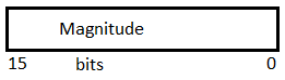
Byte and UInt8 are 1-byte (8-bit) unsigned positive integer numbers. The Magnitude occupies all 8-bits.

Word and UInt16
Word and UInt16 are 2-byte (16-bit) unsigned integer numbers.
FixedUInt, Cardinal and UInt32
FixedUInt, Cardinal, and UInt32 are 4-byte (32-bit) unsigned integer numbers.

UInt64
UInt64 are 8-byte (64-bit) unsigned integer numbers.

Platform-Independent Signed Integer Types
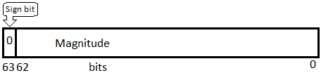
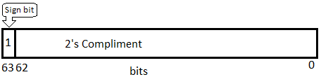
Values of signed integer types represent a sign of a number by one leading sign bit, expressed by the most significant bit. The sign bit is 0 for a positive number, and 1 for a negative number. Other bits in a positive signed integer number are occupied by the magnitude. In a negative signed integer number, other bits are occupied by the two’s complement representation of the magnitude of the value (absolute value).
To obtain the two’s complement to a magnitude:
- Starting from the right, find the first ‘1’.
- Invert all of the bits to the left of that one.
For example:
| Example 1 | Example 2 | |
|---|---|---|
| Magnitude | 0101010
|
1010101
|
|
2’s Complement |
1010110
|
0101011
|
ShortInt, Int8
Shortint and Int8 are 1-byte (8-bit) signed integer numbers. The sign bit’ occupies the most significant 7-th bit, the Magnitude or two’s complement occupies other 7 bits.


SmallInt and Int16
SmallInt and Int16 are 2-byte (16-bit) signed integer numbers.


FixedInt, Integer and Int32
FixedInt, Integer, and Int32 are 4-byte (32-bit) signed integer numbers.


Int64
Int64 are 8-byte (64-bit) signed integer numbers.
Platform-Dependent Integer Types
The platform-dependent integer types are transformed to fit the bit size of the current target platform. On 64-bit platforms they occupy 64 bits, on 32-bit platforms they occupy 32 bits (except the LongInt and LongWord types).
When the size of the target platform is the same as the CPU platform, then one platform-dependent integer number exactly matches the size of CPU registers. These types are often used when best performance is desired for a particular CPU type and operating system.
Unsigned Integer NativeUInt
NativeUInt is the platform-dependent unsigned integer type. The size and internal representation of NativeUInt depends on the current platform. On 32-bit platforms, NativeUInt is equivalent to the Cardinal type. On 64-bit platforms, NativeUInt is equivalent to the UInt64 type.
Signed Integer NativeInt
NativeInt is the platform-dependent signed integer type. The size and internal representation of NativeInt depends on the current platform. On 32-bit platforms, NativeInt is equivalent to the Integer type. On 64-bit platforms, NativeInt is equivalent to the Int64 type.
LongInt and LongWord
LongInt defines the signed integer type and the LongWord defines the unsigned integer type.
LongInt and LongWord platform dependent integer types size are changed on each platforms, except for 64-bit Windows that remains unchanged (32-bits).
| Size | ||
|---|---|---|
| 32-bit platforms and 64-bit Windows platforms | 64-bit iOS platforms | |
| LongInt | 32-bits (4 bytes) | 64-bits (8 bytes) |
|
LongWord |
32-bits (4 bytes) | 64-bits (8 bytes) |
Note: 32-bit platforms in RAD Studio include 32-bit Windows, 32-bit macOS, 32-bit iOS, and Android.
On 64-bit iOS platforms, if you want to use:
-
- 32-bits signed integer type, use Integer or FixedInt instead of LongInt.
- 32-bits unsigned integer type, use Cardinal or FixedUInt instead of LongWord.
Integer Subrange Types
When you use integer constants to define the minimum and maximum bounds of a subrange type, you define an integer subrange type. An integer subrange type represents a subset of the values in an integer type (called the base type). The base type is the smallest integer type that contains the specified range (contains both the minimum and maximum bounds).
The internal data format of an integer subrange type variable depends on its minimum and maximum bounds:
- If both bounds are within the range -128..127 (ShortInt), the variable is stored as a signed byte.
- If both bounds are within the range 0..255 (Byte), the variable is stored as an unsigned byte.
- If both bounds are within the range -32768..32767 (SmallInt), the variable is stored as a signed word.
- If both bounds are within the range 0..65535 (Word), the variable is stored as an unsigned word.
- If both bounds are within the range -2147483648..2147483647 (FixedInt and LongInt on 32-bit platforms and 64-bit Windows platforms), the variable is stored as a signed double word.
- If both bounds are within the range 0..4294967295 (FixedUInt and LongWord on 32-bit platforms and 64-bit Windows platforms), the variable is stored as an unsigned double word.
- If both bounds are within the range -2^63..2^63-1 (Int64 and LongInt on 64-bit iOS platforms), the variable is stored as a signed quadruple word.
- If both bounds are within the range 0..2^64-1 (UInt64 and LongWord on 64-bit iOS platforms), the variable is stored as an unsigned quadruple word.
Note: A «word» occupies two bytes.
Character Types
On the 32-bit and 64-bit platforms:
- Char and WideChar are stored as an unsigned word variable, normally using UTF-16 or Unicode encoding.
- AnsiChar type is stored as an unsigned byte. In Delphi 2007 and earlier, Char was represented as an AnsiChar. The character type used with Short Strings is always AnsiChar and is stored in unsigned byte values.
- The default long string type (string) is now UnicodeString, which is reference counted like an AnsiString, the former default long string type. Compatibility with older code may require the use of the AnsiString type.
- WideString is composed of WideChars like UnicodeString, but is not reference counted.
Boolean Types
A Boolean type is stored as a Byte, a ByteBool is stored as a Byte, a WordBool type is stored as a Word, and a LongBool is stored as a Longint.
A Boolean can assume the values 0 (False) and 1 (True). ByteBool, WordBool, and LongBool types can assume the values 0 (False) or nonzero (True).
Enumerated Types
An enumerated type is stored as an unsigned byte if the enumeration has no more than 256 values and the type was declared in the {$Z1} state (the default). If an enumerated type has more than 256 values, or if the type was declared in the {$Z2} state, it is stored as an unsigned word. If an enumerated type is declared in the {$Z4} state, it is stored as an unsigned double-word.
Real Types
The real types store the binary representation of a sign (+ or -), an exponent, and a significand. A real value has the form
+/- significand * 2^exponent
where the significand has a single bit to the left of the binary decimal point (that is, 0 <= significand < 2).
In the images that follow, the most significant bit is always on the left, and the least significant bit, on the right. The numbers at the top indicate the width (in bits) of each field, with the leftmost items stored at the highest addresses. For example, for a Real48 value, e is stored in the first byte, f in the following five bytes, and s in the most significant bit of the last byte.
The Real48 type
On the 32-bit and 64-bit platforms, a 6-byte (48-bit) Real48 number is divided into three fields.
If 0 < e <= 255, the value v of the number is given by:
v = (-1)s * 2(e-129) * (1.f)
If e = 0, then v = 0.
The Real48 type cannot store denormals, NaNs, and infinities (Inf). Denormals become zero when stored in a Real48, while NaNs and infinities produce an overflow error if an attempt is made to store them in a Real48.
The Single type
On 32-bit and 64-bit platforms, a 4-byte (32-bit) Single number is divided into three fields.
The value v of the number is given by:
- If
0 < e < 255, thenv = (-1)s * 2(e-127) * (1.f)
- If
e = 0andf <> 0, thenv = (-1)s * 2(-126) * (0.f)
- If
e = 0andf = 0, thenv = (-1)s * 0
- If
e = 255andf = 0, thenv = (-1)s * Inf
- If
e = 255andf <> 0, thenvis a NaN
The Double type
The Real type, in the current implementation, is equivalent to Double.
On 32-bit and 64-bit platforms, an 8-byte (64-bit) Double number is divided into three fields.
The value v of the number is given by:
- If
0 < e < 2047, thenv = (-1)s * 2(e-1023) * (1.f)
- If
e = 0andf <> 0, thenv = (-1)s * 2(-1022) * (0.f)
- If
e = 0andf = 0, thenv = (-1)s * 0
- If
e = 2047andf = 0, thenv = (-1)s * Inf
- If
e = 2047andf <> 0, thenvis a NaN
The Extended type
Extended offers greater precision on 32-bit Intel platform than other real types, but is less portable. Be careful using Extended if you are creating data files to share across platforms. Be aware that:
On 32-bit Intel platform, an Extended number is represented as 10 bytes (80 bits). An Extended number is divided into four fields.
The value v of the number is given by:
- If
0 <= e < 32767, thenv = (-1)s * 2(e-16383) * (i.f) - If
e = 32767andf = 0, thenv = (-1)s * Inf - If
e = 32767andf <> 0, thenvis a NaN
However, on the 64-bit Intel platform and ARM platform, the Extended type is an alias for Double, which is only 8 bytes. This difference can adversely affect numeric precision in floating-point operations. For more information, see Delphi Considerations for Multi-Device Applications.
The Comp type
An 8-byte (64-bit) Comp number is stored as a signed 64-bit integer.
The Currency type
An 8-byte (64-bit) Currency number is stored as a scaled and signed 64-bit integer with the 4 least significant digits implicitly representing 4 decimal places.
Pointer Types
On 32-bit platforms, a pointer type is stored in 4 bytes as a 32-bit address.
On 64-bit platforms, a pointer type is stored in 8 bytes as a 64-bit address.
The pointer value nil is stored as zero.
Short String Types
A ShortString string occupies as many bytes as its maximum length plus one. The first byte contains the current dynamic length of the string, and the following bytes contain the characters of the string.
The length byte and the characters are considered unsigned values. The maximum string length is 255 characters plus a length byte (string[255]).
Long String Types
A string variable of type UnicodeString or AnsiString occupies 4 bytes of memory on 32-bit platforms (and 8 bytes on 64-bit) that contain a pointer to a dynamically allocated string. When a string variable is empty (contains a zero-length string), the string pointer is nil and no dynamic memory is associated with the string variable. For a nonempty string value, the string pointer points to a dynamically allocated block of memory that contains the string value in addition to information describing the string. The tables below show the layout of a long-string memory block.
Format of UnicodeString data type (32-bit and 64-bit)
| Field | CodePage | ElementSize | ReferenceCount | Length | String Data (ElementSized) |
Null Term |
|---|---|---|---|---|---|---|
|
Offset |
|
|
|
|
|
|
|
Contents |
16-bit codepage of string data |
16-bit element size of string data |
32-bit reference-count |
Length in characters |
Character string of ElementSized data |
NULL character |
Numbers in the Offset row show offsets of fields, describing the string contents, from the string pointer, which points to the String Data field (offset = 0), containing a block of memory that contains the actual string values.
The NULL character at the end of a string memory block is automatically maintained by the compiler and the built-in string handling routines. This makes it possible to typecast a string directly to a null-terminated string.
See also «New String Type: UnicodeString.»
For string literals, the compiler generates a memory block with the same layout as a dynamically allocated string, but with a reference count of -1. String constants are treated the same way, the only difference from literals being that they are a pointer to a -1 reference counter block.
When a pointer to a string structure (source) is assigned to a string variable (destination), the reference counter dictates how this is done. Usually, the reference count is decreased for the destination and increased for the source, as both pointers, source and destination, will point to the same memory block after the assignment.
If the source reference count is -1 (string constant), a new structure is created with a reference count of 1. If the destination is not nil, the reference counter is decreased. If it reaches 0, the structure is deallocated from the memory. If the destination is nil, no additional actions are taken for it.
The destination will then point to the new structure.
var
 destination : String;
 source : String;
...
destination := 'qwerty';  // reference count for the newly-created block of memory (containing the 'qwerty' string) pointed at by the "destination" variable is now 1
...
source := 'asdfgh'; // reference count for the newly-created block of memory (containing the 'asdfgh' string) pointed at by the "destination" variable is now 1
destination := source; // reference count for the memory block containing the 'asdfgh' string is now 2, and since reference count for the block of memory containing the 'qwerty' string is now 0, the memory block is deallocated.
If the source reference count is not -1, it is incremented and the destination will point to it.
var
  destination, destination2, destination3: String;
  destination := 'Sample String'; //reference count for the newly-created block of memory containing 'Sample string' is 1.
  destination2 := destination; //reference count for the block of memory containing 'Sample string' is now 2.
  destination3 := destination; //reference count for the block of memory containing 'Sample string' is now 3.
Note: No string variable can point to a structure with a reference count of 0. Structures are always deallocated when they reach 0 reference count and cannot be modified when they have -1 reference count.
Wide String Types
On 32-bit platforms, a wide string variable occupies 4 bytes of memory (and 8 bytes on 64-bit) that contain a pointer to a dynamically allocated string. When a wide string variable is empty (contains a zero-length string), the string pointer is nil and no dynamic memory is associated with the string variable. For a nonempty string value, the string pointer points to a dynamically allocated block of memory that contains the string value in addition to a 32-bit length indicator. The table below shows the layout of a wide string memory block on Windows.
Wide string dynamic memory layout (32-bit and 64-bit)
|
Offset |
|
|
|
|
Contents |
32-bit length indicator |
Character string |
NULL character |
The string length is the number of bytes, so it is twice the number of wide characters contained in the string.
The NULL character at the end of a wide string memory block is automatically maintained by the compiler and the built-in string handling routines. This makes it possible to typecast a wide string directly to a null-terminated string.
Set Types
A set is a bit array where each bit indicates whether an element is in the set or not. The maximum number of elements in a set is 256, so a set never occupies more than 32 bytes. The number of bytes occupied by a particular set is equal to
(Max div 8) - (Min div 8) + 1
where Max and Min are the upper and lower bounds of the base type of the set. The byte number of a specific element E is
(E div 8) - (Min div 8)
and the bit number within that byte is
E mod 8
where E denotes the ordinal value of the element. When possible, the compiler stores sets in CPU registers, but a set always resides in memory if it is larger than the platform-dependent integer type or if the program contains code that takes the address of the set.
Static Array Types
The memory that a static-array variable occupies is defined by the calculation of Length(array) * SizeOf(array[Low(array)]) in bytes. The static-array variable is entirely allocated as part of the parent data structure. A static array is stored as a contiguous sequence of elements of the component type of the array. The components with the lowest indexes are stored at the lowest memory addresses. A multidimensional array is stored with the rightmost dimension increasing first.
Dynamic Array Types
On the 32-bit platform, a dynamic-array variable occupies 4 bytes of memory (and 8 bytes on 64-bit) that contain a pointer to the dynamically allocated array. When the variable is empty (uninitialized) or holds a zero-length array, the pointer is nil and no dynamic memory is associated with the variable. For a nonempty array, the variable points to a dynamically allocated block of memory that contains the array in addition to a 32-bit (64-bit on Win64) length indicator and a 32-bit reference count. The table below shows the layout of a dynamic-array memory block.
Dynamic array memory layout (32-bit and 64-bit)
|
Offset 32-bit |
|
|
|
|
Offset 64-bit |
|
|
|
|
Contents |
32-bit reference-count |
32-bit or 64-bit on 64-bit platform |
Array elements |
Record Types
When a record type is declared in the {$A+} state (the default), and when the declaration does not include a packed modifier, the type is an unpacked record type, and the fields of the record are aligned for efficient access by the CPU, and according to the platform. The alignment is controlled by the type of each field. Every data type has an inherent alignment, which is automatically computed by the compiler. The alignment can be 1, 2, 4, or 8, and represents the byte boundary on which a value of the type must be stored in order to provide the most efficient access. The table below lists the alignments for all data types.
Type alignment masks (32-bit only)
| Type | Alignment |
|---|---|
|
Ordinal types |
Size of the type (1, 2, 4, or |
|
Real types |
2 for Real48, 4 for Single, 8 for Double and Extended |
|
Short string types |
1 |
|
Array types |
Same as the element type of the array |
|
Record types |
The largest alignment of the fields in the record |
|
Set types |
Size of the type if 1, 2, or 4, otherwise 1 |
|
All other types |
Determined by the $A directive |

To ensure proper alignment of the fields in an unpacked record type, the compiler inserts an unused byte before fields with an alignment of 2, and up to 3 unused bytes before fields with an alignment of 4, if required. Finally, the compiler rounds the total size of the record upward to the byte boundary specified by the largest alignment of any of the fields.
Implicit Packing of Fields with a Common Type Specification
Earlier versions of the Delphi compiler, such as Delphi 7 and earlier, implicitly applied packed alignment to fields that were declared together, that is, fields that have a common type specification. Newer compilers can reproduce the behavior if you specify the directive {$OLDTYPELAYOUT ON}. This directive byte-aligns (packs) the fields that have a common type specification, even if the declaration does not include the packed modifier and the record type is not declared in the {$A-} state.
Thus, for example, given the following declaration:
 {$OLDTYPELAYOUT ON}
 type
   TMyRecord = record
     A, B: Extended;
     C: Extended;
   end;
 {$OLDTYPELAYOUT OFF}
A and B are packed (aligned on byte boundaries) because the {$OLDTYPELAYOUT ON} directive is specified and because A and B share the same type specification. However, for the separately declared C field, the compiler uses the default behavior and pads the structure with unused bytes to ensure the field appears on a quadword boundary.
When a record type is declared in the {$A-} state, or when the declaration includes the packed modifier, the fields of the record are not aligned, but are instead assigned consecutive offsets. The total size of such a packed record is simply the size of all the fields. Because data alignment can change, it is a good idea to pack any record structure that you intend to write to disk or pass in memory to another module compiled using a different version of the compiler.
File Types
File types are represented as records. Typed files and untyped files occupy 592 bytes on 32-bit platforms and 616 bytes on 64-bit platforms, which are laid out as follows:
 type
   TFileRec = packed record
     Handle: NativeInt;
     Mode: word;
     Flags: word;
     case Byte of
       0: (RecSize: Cardinal);
       1: (BufSize: Cardinal;
    	   BufPos: Cardinal;
    	   BufEnd: Cardinal;
    	   BufPtr: _PAnsiChr;
    	   OpenFunc: Pointer;
    	   InOutFunc: Pointer;
    	   FlushFunc: Pointer;
    	   CloseFunc: Pointer;
    	   UserData: array[1..32] of Byte;
    	   Name: array[0..259] of WideChar; );
  end;
Text files occupy 730 bytes on Win 32 and 754 bytes on Win64, which are laid out as follows:
 type
   TTextBuf = array[0..127] of Char;
   TTextRec = packed record
     Handle: NativeInt;
     Mode: word;
     Flags: word;
     BufSize: Cardinal;
     BufPos: Cardinal;
     BufEnd: Cardinal;
     BufPtr: _PAnsiChr;
     OpenFunc: Pointer;
     InOutFunc: Pointer;
     FlushFunc: Pointer;
     CloseFunc: Pointer;
     UserData: array[1..32] of Byte;
     Name: array[0..259] of WideChar;
     Buffer: TTextBuf; //
     CodePage: Word;
     MBCSLength: ShortInt;
     MBCSBufPos: Byte;
     case Integer of
       0: (MBCSBuffer: array[0..5] of _AnsiChr);
       1: (UTF16Buffer: array[0..2] of WideChar);
   end;
Handle contains the handle of the file (when the file is open).
The Mode field can assume one of the values:
 const
   fmClosed = $D7B0;
   fmInput= $D7B1;
   fmOutput = $D7B2;
   fmInOut= $D7B3;
where fmClosed indicates that the file is closed, fmInput and fmOutput indicate a text file that has been reset (fmInput) or rewritten (fmOutput), fmInOut indicates a typed or untyped file that has been reset or rewritten. Any other value indicates that the file variable is not assigned (and hence not initialized).
The UserData field is available for user-written routines to store data in.
Name contains the file name, which is a sequence of characters terminated by a null character (#0).
For typed files and untyped files, RecSize contains the record length in bytes, and the Private field is unused but reserved.
For text files, BufPtr is a pointer to a buffer of BufSize bytes, BufPos is the index of the next character in the buffer to read or write, and BufEnd is a count of valid characters in the buffer. OpenFunc, InOutFunc, FlushFunc, and CloseFunc are pointers to the I/O routines that control the file; see Device functions. Flags determines the line break style as follows.
|
bit 0 clear |
LF line breaks |
|
bit 0 set |
CRLF line breaks |
All other Flags bits are reserved for future use.
Note: For using the UnicodeString type (the default Delphi string type), the various stream types in the Classes unit (TFileStream, TStreamReader, TStreamWriter, and so forth) are more useful, since the older file types have limited Unicode functionality, particularly the old text file type.
Procedural Types
On the 32-bit platform, a procedure pointer is stored as a 32-bit pointer to the entry point of a procedure or function. A method pointer is stored as a 32-bit pointer to the entry point of a method, followed by a 32-bit pointer to an object.
On the 64-bit platform, a procedure pointer is stored as a 64-bit pointer to the entry point of a procedure or function. A method pointer is stored as a 64-bit pointer to the entry point of a method, followed by a 64-bit pointer to an object.
Class Types
On the 32-bit platforms (Win32, macOS, iOS and Android), a class-type value is stored as a 32-bit pointer to an instance of the class (and as a 64-bit pointer on the 64-bit platform), which is called an object. The internal data format of an object resembles that of a record. The fields of the object are stored in order of declaration as a sequence of contiguous variables. Fields are always aligned, corresponding to an unpacked record type. Therefore, the alignment corresponds to the largest alignment of the fields in the object. Any fields inherited from an ancestor class are stored before the new fields defined in the descendent class.
On the 32-bit platforms, the first 4-byte field of every object (the first 8-byte field on the 64-bit platform) is a pointer to the virtual method table (VMT) of the class. There is exactly one VMT per class (not one per object); distinct class types, no matter how similar, never share a VMT. VMTs are built automatically by the compiler, and are never directly manipulated by a program. Pointers to VMTs, which are automatically stored by constructor methods in the objects they create, are also never directly manipulated by a program.
The layout of a VMT is shown in the following table. On the 32-bit platforms, at positive offsets, a VMT consists of a list of 32-bit method pointers (64-bit method pointers on the 64-bit platform)—one per user-defined virtual method in the class type—in order of declaration. Each slot contains the address of the corresponding entry point of the virtual method. This layout is compatible with a C++ v-table and with COM. At negative offsets, a VMT contains a number of fields that are internal to Delphi’s implementation. Applications should use the methods defined in TObject to query this information, since the layout is likely to change in future implementations of the Delphi language.
Virtual method table layout
| Offset Win32, macOS |
Offset Win64 |
Offset iOS/ARM, Android/ARM |
Type | Description | Constant in System.pas |
|---|---|---|---|---|---|
|
-88 |
-200 |
-108 |
Pointer |
Pointer to virtual method table (or nil) |
vmtSelfPtr |
|
-84 |
-192 |
-104 |
Pointer |
Pointer to interface table (or nil) |
vmtIntfTable |
|
-80 |
-184 |
-100 |
Pointer |
Pointer to Automation information table (or nil) |
vmtAutoTable |
|
-76 |
-176 |
-96 |
Pointer |
Pointer to instance initialization table (or nil) |
vmtInitTable |
|
-72 |
-168 |
-92 |
Pointer |
Pointer to type information table (or nil) |
vmtTypeInfo |
|
-68 |
-160 |
-88 |
Pointer |
Pointer to field definition table (or nil) |
vmtFieldTable |
|
-64 |
-152 |
-84 |
Pointer |
Pointer to method definition table (or nil) |
vmtMethodTable |
|
-60 |
-144 |
-80 |
Pointer |
Pointer to dynamic method table (or nil) |
vmtDynamicTable |
|
-56 |
-136 |
-76 |
Pointer |
Pointer to short string containing class name |
vmtClassName |
|
-52 |
-128 |
-72 |
Cardinal |
Instance size in bytes |
vmtInstanceSize |
|
-48 |
-120 |
-68 |
Pointer |
Pointer to a pointer to ancestor class (or nil) |
vmtParent |
|
n/a |
n/a |
-64 |
Pointer |
Entry point of __ObjAddRef method |
vmtObjAddRef |
|
n/a |
n/a |
-60 |
Pointer |
Entry point of __ObjRelease method |
vmtObjRelease |
|
-44 |
-112 |
-56 |
Pointer |
Entry point of Equals method |
vmtEquals |
|
-40 |
-104 |
-52 |
Pointer |
Entry point of GetHashCode method |
vmtGetHashCode |
|
-36 |
-96 |
-48 |
Pointer |
Entry point of ToString method |
vmtToString |
|
-32 |
-88 |
-44 |
Pointer |
Pointer to entry point of SafecallException method (or nil) |
vmtSafeCallException |
|
-28 |
-80 |
-40 |
Pointer |
Entry point of AfterConstruction method |
vmtAfterConstruction |
|
-24 |
-72 |
-36 |
Pointer |
Entry point of BeforeDestruction method |
vmtBeforeDestruction |
|
-20 |
-64 |
-32 |
Pointer |
Entry point of Dispatch method |
vmtDispatch |
|
-16 |
-56 |
-28 |
Pointer |
Entry point of DefaultHandler method |
vmtDefaultHandler |
|
-12 |
-48 |
-24 |
Pointer |
Entry point of NewInstance method |
vmtNewInstance |
|
-8 |
-40 |
-20 |
Pointer |
Entry point of FreeInstance method |
vmtFreeInstance |
|
-4 |
-32 |
-16 |
Pointer |
Entry point of Destroy destructor |
vmtDestroy |
|
0 |
0 |
0 |
Pointer |
Entry point of first user-defined virtual method |
|
|
4 |
8 |
4 |
Pointer |
Entry point of second user-defined virtual method |
Class Reference Types
On the 32-bit (Win32, macOS, iOS and Android) platform, a class-reference value is stored as a 32-bit pointer to the virtual method table (VMT) of a class.
On the 64-bit (Win64) platform, a class-reference value is stored as a 64-bit pointer to the virtual method table (VMT) of a class.
Variant Types
Variants rely on boxing and unboxing of data into an object wrapper, as well as Delphi helper classes to implement the variant-related RTL functions.
On the 32-bit platform, a variant is stored as a 16-byte record that contains a type code and a value (or a reference to a value) of the type given by the code. On the 64-bit platform, a variant is stored as a 24-byte record. The System and System.Variants units define constants and types for variants.
The TVarData type represents the internal structure of a Variant variable (on Windows, this is identical to the Variant type used by COM and the Win32 API). The TVarData type can be used in typecasts of Variant variables to access the internal structure of a variable. The TVarData record contains the following fields:
- The VType field of the TVarType type has the Word (16-bit) size. VType contains the type code of the variant in the lower 12 bits (the bits defined by the varTypeMask
= $FFFconstant). In addition, the varArray= $2000bit may be set to indicate that the variant is an array, and the varByRef (= $4000) bit may be set to indicate that the variant contains a reference as opposed to a value. - The Reserved1, Reserved2, and Reserved3 (Word size) fields are unused.
The contents of the remaining 8 bytes (32-bit platform) or 16 bytes (64-bit platform) of a TVarData record depend on the VType field as follows:
- If neither the varArray nor the varByRef bits are set, the variant contains a value of the given type.
- If the varArray bit is set, the variant contains a pointer to a TVarArray structure that defines an array. The type of each array element is given by the varTypeMask bits in the VType field.
- If the varByRef bit is set, the variant contains a reference to a value of the type given by the varTypeMask and varArray bits in the VType field.
The varString type code is private. Variants containing a varString value should never be passed to a non-Delphi function. On the Windows platform, Delphi’s Automation support automatically converts varString variants to varOleStr variants before passing them as parameters to external functions.
See Also
- Memory Management
- 64-bit Windows Data Types Compared to 32-bit Windows Data Types
- About Data Types (Delphi)
- String Types (Delphi)
- Structured Types (Delphi)
Урок 1. Типы данных
языка программирования Turbo Pascal 7.0
-
Определение типов данных.
-
Целочисленный тип данных, их
количество и диапазон значений. -
Преобразование целых типов.
Практический пример.
-
Определение типов
данных
Тип
данных языка программирования TP 7.0 определяет:
-
формат данных в памяти
компьютера; -
множество допустимых значений,
которые может принимать принадлежащая к выбранному типу переменная или
константа; -
множество допустимых операций,
применимых к этому типу.
Множество типов
языка TP 7.0 разделяют на две группы — стандартные
(предопределенные) и определяемые пользователем (пользовательские).
К стандартным типам языка
программирования TP 7.0 относят такие типы данных как:
числовые — группа целых (целочисленных) и группа вещественных (дробных)
переменных, логические (булевские) переменные, символьные, указательные и
текстовые.
2. Целочисленный тип данных
(группа целых типов)
В TP 7.0
определено пять целочисленных типов: Integer
(целое), Sortint (короткое целое), Longint (длинное целое), Byte (байт), Word
(слово), диапазон допустимых значений которых приведен в таблице 1.
Таблица 1
|
Тип |
Наименование типа |
Диапазон значений |
Длина (байт) |
|
Shortint |
Короткое |
-128 —:- 127 (-27 -:- 27 — 1) |
1 |
|
Integer |
Целое |
-32768 -:- 32767 (-215 -:- 215 -1) |
2 |
|
Longint |
Длинное |
-2147483648 -:- 2147683647 (-231 -:- 231 -1) |
4 |
|
Byte |
Байт |
0 -:- 255 |
1 |
|
Word |
Слово |
0 -:- 6553 |
2 |
В TP 7.0
любое значение, относящееся к целочисленному типу, должно быть написано в виде
целого числа, например, a:=125;
b:=5; (переменным a и b присвоены значения целых чисел
125, 5 соответственно). В случае, когда результат расчетов выходит за пределы
допустимых значений указанного типа индикации ошибки может и не быть, но может
напечатан неверный результат.
В ОЗУ компьютера числовые значения
целых переменных представлены в виде двоичных цифр, которые называются битами
(BInary digiT — BIT). ОЗУ компьютера представляет собой техническое
устройство, состоящее из набора адресуемых ячеек памяти, позволяющих запомнить 8
bit (двоичных цифр).
Определение. Группа из
восьми соседних разрядов (битов), с которыми оперирует компьютер при хранении,
передаче и обработке информации называется байтом.
Конструкция,
состоящая из 2- х байт, называется словом, из 4-х — двойным
словом.
|
1 |
1 |
1 |
1 |
1 |
1 |
1 |
1 |
… |
0 |
1 |
1 |
1 |
1 |
1 |
1 |
1 |
-128 127
На рисунке представлен диапазон
целых чисел типа shortint (короткое целое) в виде
записи двоичными цифрами в разрядной сетке величиной 1 байт. Серым цветом
помечен знаковый разряд 0 — определяет знак +, 1 — определяет знак —
.
3. Преобразование целых
типов
Типы
целочисленных значений могут быть преобразованы друг в друга функциями
преобразования, которые имеют названия соответствующих типов и имеют следующий
формат:
<Наименование целочисленного
типа>(n)
где <Наименование
целочисленного типа> — shortint,
integer, longint, byte,
word;
n — целая
переменная, которая может быть задано явно или вычислена в программе.
Приведенная ниже программа
иллюстрирует пребразование целого числа типа longint вводимого с клавиатуры, в другие
целочисленные типы.
{Преобразование целых типов}
Program vv3;
Uses Crt; {Вызов библиотечного модуля работы с
дисплеем}
Var j,k: longint; {Описание переменных,
используемых в пр-ме}
begin
ClrScr;{Процедура очистки экрана
дисплея}
Write(‘Введи целое число: ‘);
ReadLn(k); {Ввод числа с
клавиатуры}
WriteLn; {Перевод строки}
{Вывод
сообщений на экран}
Write(‘Если введенное число входит в диапазон
типа,’);
WriteLn(‘то оно будет равно
выводимому’);
WriteLn;
WriteLn(‘Вывод числа на
дисплей’);
{Преобразование в тип Byte}
j:=Byte(k);
WriteLn(‘ Тип Byte = ‘,j);
{Преобразование в тип Word}
j:=Word(k);
WriteLn(‘ Тип Word = ‘,j);
{Преобразование в тип Shortint}
j:=Shortint(k);
WriteLn(‘ Тип Sortint = ‘,j);
{Преобразование в тип Integer}
j:=Integer(k);
WriteLn(‘ Тип Integer = ‘,j);
{Преобразование в тип longint}
j:=Longint(k);
WriteLn(‘ Тип Longint = ‘,j);
{}
ReadKey; {Ожидание нажатия любой
клавиши}
end.
Если введенное
число входит в диапазон типа целого числа, то оно будет равно выводимому. При
решении вычислительных задач следует учитывать, что при выходе результата
вычислений из диапазона целочисленного типа, индикации ошибки на экране дисплея
может и не быть. Поэтому необходимо проверять результат вычислений на
минимальных и максимальных значениях аргумента.