
Программное создание графика (диаграммы) в VBA Excel с помощью метода Charts.Add на основе данных из диапазона ячеек на рабочем листе. Примеры.
Метод Charts.Add
В настоящее время на сайте разработчиков описывается метод Charts.Add2, который, очевидно, заменил метод Charts.Add. Тесты показали, что Charts.Add продолжает работать в новых версиях VBA Excel, поэтому в примерах используется именно он.
Синтаксис
|
Charts.Add ([Before], [After], [Count]) |
|
Charts.Add2 ([Before], [After], [Count], [NewLayout]) |
Параметры
Параметры методов Charts.Add и Charts.Add2:
| Параметр | Описание |
|---|---|
| Before | Имя листа, перед которым добавляется новый лист с диаграммой. Необязательный параметр. |
| After | Имя листа, после которого добавляется новый лист с диаграммой. Необязательный параметр. |
| Count | Количество добавляемых листов с диаграммой. Значение по умолчанию – 1. Необязательный параметр. |
| NewLayout | Если NewLayout имеет значение True, диаграмма вставляется с использованием новых правил динамического форматирования (заголовок имеет значение «включено», а условные обозначения – только при наличии нескольких рядов). Необязательный параметр. |
Если параметры Before и After опущены, новый лист с диаграммой вставляется перед активным листом.
Примеры
Таблицы
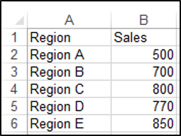
В качестве источников данных для примеров используются следующие таблицы:

Пример 1
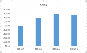
Программное создание объекта Chart с типом графика по умолчанию и по исходным данным из диапазона «A2:B26»:
|
Sub Primer1() Dim myChart As Chart ‘создаем объект Chart с расположением нового листа по умолчанию Set myChart = ThisWorkbook.Charts.Add With myChart ‘назначаем объекту Chart источник данных .SetSourceData (Sheets(«Лист1»).Range(«A2:B26»)) ‘переносим диаграмму на «Лист1» (отдельный лист диаграммы удаляется) .Location xlLocationAsObject, «Лист1» End With End Sub |
Результат работы кода VBA Excel из первого примера:

Пример 2
Программное создание объекта Chart с двумя линейными графиками по исходным данным из диапазона «A2:C26»:
|
Sub Primer2() Dim myChart As Chart Set myChart = ThisWorkbook.Charts.Add With myChart .SetSourceData (Sheets(«Лист1»).Range(«A2:C26»)) ‘задаем тип диаграммы (линейный график с маркерами) .ChartType = xlLineMarkers .Location xlLocationAsObject, «Лист1» End With End Sub |
Результат работы кода VBA Excel из второго примера:

Пример 3
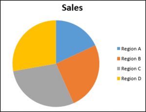
Программное создание объекта Chart с круговой диаграммой, разделенной на сектора, по исходным данным из диапазона «E2:F7»:
|
Sub Primer3() Dim myChart As Chart Set myChart = ThisWorkbook.Charts.Add With myChart .SetSourceData (Sheets(«Лист1»).Range(«E2:F7»)) ‘задаем тип диаграммы (пирог — круг, разделенный на сектора) .ChartType = xlPie ‘задаем стиль диаграммы (с отображением процентов) .ChartStyle = 261 .Location xlLocationAsObject, «Лист1» End With End Sub |
Результат работы кода VBA Excel из третьего примера:

Примечание
В примерах использовались следующие методы и свойства объекта Chart:
| Компонент | Описание |
|---|---|
| Метод SetSourceData | Задает диапазон исходных данных для диаграммы. |
| Метод Location | Перемещает диаграмму в заданное расположение (новый лист, существующий лист, элемент управления). |
| Свойство ChartType | Возвращает или задает тип диаграммы. Смотрите константы. |
| Свойство ChartStyle | Возвращает или задает стиль диаграммы. Значение нужного стиля можно узнать, записав макрос. |
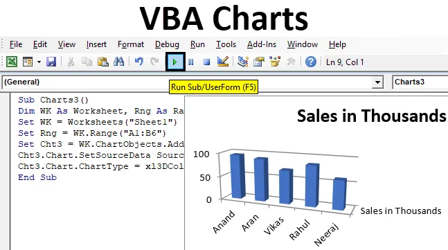
VBA stands for Visual Basic for Applications and it is developed by Microsoft. MS Excel and many other Microsoft applications like word, access, etc have this language integrated into them using which one can do various things. VBA can be used in MS Excel through the code editor in its developer tab through which one can generate various types of charts and user-defined functions, connect to windows APIs, and much more.
Enabling the Developer Tab in Excel
To use VBA in excel first of all we will need to make the developer tab visible as it is not visible as default when it is installed. We can do this by following the steps below:
Step 1: Click on the file option in the top left corner.

Step 2: Click on the options tab in the bottom left corner which will take you to excel options.

Step 3: Then click on the customize ribbon option and check the developer tab in the options available.

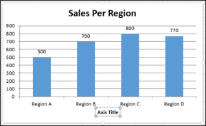
Table of Data for Charts
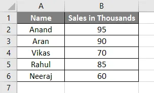
The table of data that I used for generating the chart is a small table containing the marks of students in different subjects. The table is shown below:

Programming Charts in Excel VBA
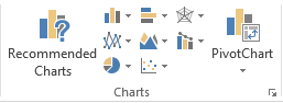
To produce charts from the data table present in our sheet first we need to create a command button by clicking which we will generate the desired chart that we programmed in the VBA. To do so just select the developer tab and then select insert then from ActiveX Controls choose the command button then place it anywhere in the sheet.

After placing the button in the sheet double click the button, if it doesn’t work then click the design mode option in the developer tab and then double-click on the button. It will take you to the VBA Editor where it will open starting with the function that handles the click function of the button you just created.

To increase the font size in the VBA Editor go to the tools tab and then the options tab and then to the editor format tab and increase the font size to your desired size. After we got our button and adjusted the font size its time to write some programs to create charts using those buttons and data tables in the sheet. Below is a VBA Code that runs when the user clicks the command Button. Remember to change to design mode to go to the editor when you click the button and turn off the design mode when you want to see the click function in action.
Private Sub CommandButton1_Click()
Dim bar_graph As ChartObject
Set bar_graph = ActiveSheet.ChartObjects.Add(Top:=Range(“E4”).Top, Left:=Range(“E4”).Left, Width:=400, Height:=300)
bar_graph.Chart.SetSourceData Worksheets(“Sheet1”).Range(“A2:C8”)
bar_graph.Chart.ChartType = xl3DColumn // Here you can choose from a variety of chart types
Worksheets(“Sheet1”).Cells(1, 1).Select // Optional
End Sub
Let’s Understand the code written above in Excel VBA:
- In the above code Lines from Private Sub CommandButton1_Click to End Sub defines the Click function on the button.
- Dim refers to Dimension and it is used to declare variables in Excel VBA.
- Above we used variable bar_graph as type ChartObject. ChartObject contains all the sheets in the workbook (i.e, both chart sheets and worksheets).
- We then set the ActiveSheet where the chart will be drawn such that its left and top corner is the E4 cell just to make sure the chart appears as close to the button and data table as possible.
- The width and Height define the width and height of the chart that will be generated.
- The chart is the function that helps create and change the type of chart in the ActiveSheet.
- We set the source data for the chart with the help of SetSourceData and give it the data from Range A2 to C8 from Sheet1.
- Using the ChartType function we can choose any kind of chart that we want to generate from the number of charts available in the list. The list of charts pops up automatically when one writes “Chart.ChartType =” in the VBA Editor.
- The last line of code is optional and selects the A1 cell after completing the function which is just the Title of the table.
There are many other ways to write the same code in Excel VBA and I have shown just a single way. With the help of variables for every function and using the keyword to change their attributes can be learned easily if one learns how to write VBA in a better way.

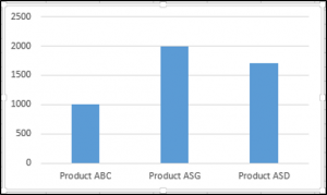
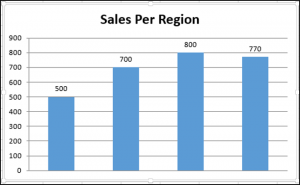
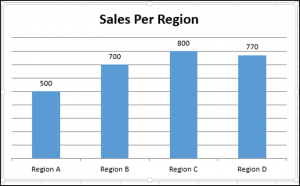
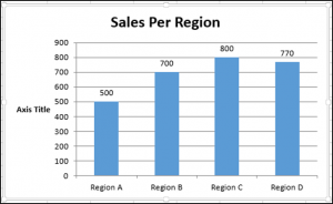
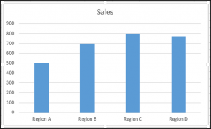
Output of Chart Function
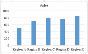
When the command button is pressed outside the design mode, the chosen chart is displayed in the cell range mentioned in the code above like the picture shown below.

Содержание
Диаграммы и графики Excel используются для визуального отображения данных. В этом руководстве мы расскажем, как использовать VBA для создания диаграмм и элементов диаграмм и управления ими.
Вы можете создавать встроенные диаграммы на листе или диаграммы на отдельных листах диаграмм.
Создание встроенной диаграммы с помощью VBA
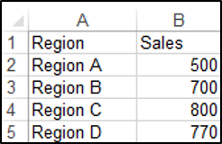
У нас есть диапазон A1: B4, который содержит исходные данные, показанные ниже:

Вы можете создать диаграмму с помощью метода ChartObjects.Add. Следующий код создаст на листе встроенную диаграмму:
| 12345678 | Sub CreateEmbeddedChartUsingChartObject ()Уменьшить размер встроенной диаграммы как ChartObjectУстановите embeddedchart = Sheets («Sheet1»). ChartObjects.Add (Left: = 180, Width: = 300, Top: = 7, Height: = 200)embeddedchart.Chart.SetSourceData Источник: = Sheets («Sheet1»). Range («A1: B4»)Конец подписки |
Результат:

Вы также можете создать диаграмму с помощью метода Shapes.AddChart. Следующий код создаст на листе встроенную диаграмму:
| 12345678 | Подложка CreateEmbeddedChartUsingShapesAddChart ()Заменить встроенную диаграмму как фигуруУстановите embeddedchart = Sheets («Sheet1»). Shapes.AddChartembeddedchart.Chart.SetSourceData Source: = Sheets («Sheet1»). Range («A1: B4»)Конец подписки |
Указание типа диаграммы с помощью VBA
У нас есть диапазон A1: B5, который содержит исходные данные, показанные ниже:

Вы можете указать тип диаграммы, используя свойство ChartType. Следующий код создаст круговую диаграмму на листе, поскольку для свойства ChartType задано значение xlPie:
| 123456789 | Sub SpecifyAChartType ()Dim chrt как ChartObjectУстановите chrt = Sheets («Sheet1»). ChartObjects.Add (Left: = 180, Width: = 270, Top: = 7, Height: = 210)chrt.Chart.SetSourceData Source: = Sheets («Sheet1»). Range («A1: B5»)chrt.Chart.ChartType = xlPieКонец подписки |
Результат:
Вот некоторые из популярных типов диаграмм, которые обычно указываются, хотя есть и другие:
- xlArea
- xlPie
- xlLine
- xlRadar
- xlXYScatter
- xlSurface
- xlBubble
- xlBarClustered
- xlColumnClustered
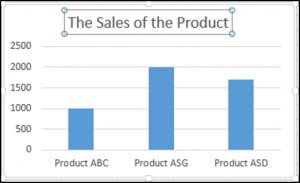
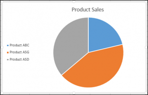
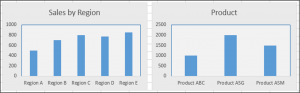
Добавление заголовка диаграммы с помощью VBA
У нас есть диаграмма, выбранная на листе, как показано ниже:

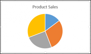
Сначала необходимо добавить заголовок диаграммы с помощью метода Chart.SetElement, а затем указать текст заголовка диаграммы, установив свойство ChartTitle.Text.
В следующем коде показано, как добавить заголовок диаграммы и указать текст заголовка активной диаграммы:
| 123456 | Sub AddingAndSettingAChartTitle ()ActiveChart.SetElement (msoElementChartTitleAboveChart)ActiveChart.ChartTitle.Text = «Продажи продукта»Конец подписки |
Результат:

Примечание. Сначала необходимо выбрать диаграмму, чтобы сделать ее активной, чтобы можно было использовать объект ActiveChart в своем коде.
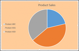
Изменение цвета фона диаграммы с помощью VBA
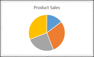
У нас есть диаграмма, выбранная на листе, как показано ниже:

Вы можете изменить цвет фона всей диаграммы, установив свойство RGB объекта FillFormat объекта ChartArea. Следующий код придаст диаграмме светло-оранжевый цвет фона:
| 12345 | Sub AddingABackgroundColorToTheChartArea ()ActiveChart.ChartArea.Format.Fill.ForeColor.RGB = RGB (253, 242, 227)Конец подписки |
Результат:

Вы также можете изменить цвет фона всей диаграммы, установив свойство ColorIndex объекта Interior объекта ChartArea. Следующий код придаст диаграмме оранжевый цвет фона:
| 12345 | Sub AddingABackgroundColorToTheChartArea ()ActiveChart.ChartArea.Interior.ColorIndex = 40Конец подписки |
Результат:
Примечание. Свойство ColorIndex позволяет указать цвет на основе значения от 1 до 56, взятого из предустановленной палитры, чтобы увидеть, какие значения представляют разные цвета, щелкните здесь.
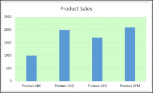
Изменение цвета области графика диаграммы с помощью VBA
У нас есть диаграмма, выбранная на листе, как показано ниже:

Вы можете изменить цвет фона только области построения диаграммы, установив свойство RGB объекта FillFormat объекта PlotArea. Следующий код придаст области построения диаграммы светло-зеленый цвет фона:
| 12345 | Sub AddingABackgroundColorToThePlotArea ()ActiveChart.PlotArea.Format.Fill.ForeColor.RGB = RGB (208, 254, 202)Конец подписки |
Результат:
Добавление легенды с помощью VBA
У нас есть диаграмма, выбранная на листе, как показано ниже:

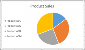
Вы можете добавить легенду с помощью метода Chart.SetElement. Следующий код добавляет легенду слева от диаграммы:
| 12345 | Подложка AddingALegend ()ActiveChart.SetElement (msoElementLegendLeft)Конец подписки |
Результат:
Вы можете указать положение легенды следующими способами:
- msoElementLegendLeft — отображает легенду в левой части диаграммы.
- msoElementLegendLeftOverlay — накладывает легенду на левую часть диаграммы.
- msoElementLegendRight — отображает легенду в правой части диаграммы.
- msoElementLegendRightOverlay — накладывает легенду на правую часть диаграммы.
- msoElementLegendBottom — отображает легенду внизу диаграммы.
- msoElementLegendTop — отображает легенду вверху диаграммы.
Добавление меток данных с помощью VBA
У нас есть диаграмма, выбранная на листе, как показано ниже:

Вы можете добавлять метки данных с помощью метода Chart.SetElement. Следующий код добавляет метки данных на внутренний конец диаграммы:
| 12345 | Sub AddingADataLabels ()ActiveChart.SetElement msoElementDataLabelInsideEndКонец подписки |
Результат:

Вы можете указать расположение меток данных следующими способами:
- msoElementDataLabelShow — отображать метки данных.
- msoElementDataLabelRight — отображает метки данных в правой части диаграммы.
- msoElementDataLabelLeft — отображает метки данных в левой части диаграммы.
- msoElementDataLabelTop — отображает метки данных вверху диаграммы.
- msoElementDataLabelBestFit — определяет наилучшее соответствие.
- msoElementDataLabelBottom — отображает метки данных внизу диаграммы.
- msoElementDataLabelCallout — отображает метки данных в виде выноски.
- msoElementDataLabelCenter — отображает метки данных в центре.
- msoElementDataLabelInsideBase — отображает метки данных на внутренней основе.
- msoElementDataLabelOutSideEnd — отображает метки данных на внешнем конце диаграммы.
- msoElementDataLabelInsideEnd — отображает метки данных на внутреннем конце диаграммы.
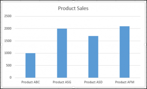
Добавление оси X и заголовка в VBA
У нас есть диаграмма, выбранная на листе, как показано ниже:

Вы можете добавить заголовок оси X и оси X с помощью метода Chart.SetElement. Следующий код добавляет к диаграмме заголовки осей X и X:
| 123456789 | Sub AddingAnXAxisandXTitle ()С ActiveChart.SetElement msoElementPrimaryCategoryAxisShow.SetElement msoElementPrimaryCategoryAxisTitleHorizontalКонец сКонец подписки |
Результат:

Добавление оси Y и заголовка в VBA
У нас есть диаграмма, выбранная на листе, как показано ниже:

Вы можете добавить заголовок оси Y и оси Y с помощью метода Chart.SetElement. Следующий код добавляет к диаграмме заголовки по осям Y и Y:
| 1234567 | Дополнительное добавлениеAYAxisandYTitle ()С ActiveChart.SetElement msoElementPrimaryValueAxisShow.SetElement msoElementPrimaryValueAxisTitleHorizontalКонец сКонец подписки |
Результат:

Изменение числового формата оси
У нас есть диаграмма, выбранная на листе, как показано ниже:

Вы можете изменить числовой формат оси. Следующий код изменяет числовой формат оси Y на валюту:
| 12345 | Sub ChangingTheNumberFormat ()ActiveChart.Axes (xlValue) .TickLabels.NumberFormat = «$ #, ## 0.00″Конец подписки |
Результат:

Изменение форматирования шрифта на диаграмме
У нас на листе выбрана следующая диаграмма, как показано ниже:

Вы можете изменить форматирование всего шрифта диаграммы, обратившись к объекту шрифта и изменив его имя, толщину и размер шрифта. Следующий код изменяет тип, вес и размер шрифта всей диаграммы.
| 12345678910 | Sub ChangingTheFontFormatting ()С ActiveChart.ChartArea.Format.TextFrame2.TextRange.Font.Name = «Times New Roman».ChartArea.Format.TextFrame2.TextRange.Font.Bold = Истина.ChartArea.Format.TextFrame2.TextRange.Font.Size = 14Конец с |
Результат:

Удаление диаграммы с помощью VBA
У нас есть диаграмма, выбранная на листе, как показано ниже:

Мы можем использовать следующий код, чтобы удалить эту диаграмму:
| 12345 | Sub DeletingTheChart ()ActiveChart.Parent.DeleteКонец подписки |
Ссылаясь на коллекцию ChartObjects
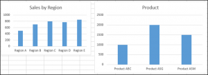
Вы можете получить доступ ко всем встроенным диаграммам на листе или в книге, обратившись к коллекции ChartObjects. У нас есть две диаграммы на одном листе, показанном ниже:

Мы обратимся к коллекции ChartObjects, чтобы дать обеим диаграммам на листе одинаковую высоту и ширину, удалить линии сетки, сделать цвет фона одинаковым, дать диаграммам одинаковый цвет области графика и сделать одинаковый цвет линии области графика. цвет:
| 12345678910111213141516 | Sub ReferringToAllTheChartsOnASheet ()Dim cht As ChartObjectДля каждого cht в ActiveSheet.ChartObjectscht.Height = 144,85cht.Width = 246,61cht.Chart.Axes (xlValue) .MajorGridlines.Deletecht.Chart.PlotArea.Format.Fill.ForeColor.RGB = RGB (242, 242, 242)cht.Chart.ChartArea.Format.Fill.ForeColor.RGB = RGB (234, 234, 234)cht.Chart.PlotArea.Format.Line.ForeColor.RGB = RGB (18, 97, 172)Следующий чтКонец подписки |
Результат:

Вставка диаграммы на отдельный лист диаграммы
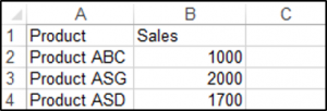
У нас есть диапазон A1: B6, который содержит исходные данные, показанные ниже:

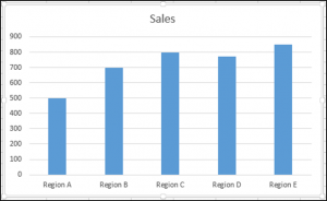
Вы можете создать диаграмму, используя метод Charts.Add. Следующий код создаст диаграмму на собственном листе диаграммы:
| 123456 | Sub InsertingAChartOnItsOwnChartSheet ()Листы («Лист1»). Диапазон («A1: B6»). ВыберитеCharts.AddКонец подписки |
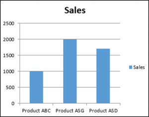
Результат:
См. Некоторые из наших других руководств по построению графиков:
Графики в Excel
Создайте гистограмму в VBA
- Графики в Excel VBA
Графики в Excel VBA
Визуализация очень важна в любых данных. В Excel, когда мы представляем данные в виде таблиц и сводной таблицы, другому пользователю может быть трудно понять основной сценарий из данных. Таким образом, в Excel у нас есть графики для представления наших данных. Диаграммы — это визуальное представление данных, представленных в строках и столбцах таблицы Excel. Теперь мы все знаем, как вставить диаграмму в таблицу Excel. В этой теме мы узнаем об использовании диаграмм в VBA. Это так же просто, как мы используем графики в Excel. Теперь, как на рабочем листе, где у нас есть различные типы графиков, аналогично, у нас есть все графики в VBA также в виде объекта. Все, что нам нужно сделать, это вызвать этот объект, чтобы использовать его. Мы можем создавать диаграммы из VBA на одном листе или на отдельном листе. Однако наиболее целесообразно использовать диаграммы на отдельном листе, чтобы избежать путаницы.
Каковы графики в VBA? Графики — это простые объекты в VBA. Мы можем сделать два типа диаграмм в VBA. Один из них известен как лист диаграммы, а другой — как встроенные диаграммы. На листе диаграммы VBA создает новый лист для диаграммы. Мы даем справочные данные, которые являются другим рабочим листом в качестве исходных данных. Теперь встроенные диаграммы — это те диаграммы, которые присутствуют в одном листе данных. Теперь кодирование для этих двух типов диаграмм немного отличается друг от друга, которое мы изучим в этой теме. Чтобы использовать свойства диаграммы в VBA, мы используем символ точки (.) В качестве IntelliSense. Теперь нам нужно помнить одну вещь: в Excel существуют различные типы графиков. Если мы не предоставляем тип диаграммы для нашего кода, VBA автоматически создает столбчатую диаграмму для нас по умолчанию. Очевидно, мы можем изменить это несколькими строками кода.
Как создать диаграммы в Excel VBA?
Теперь давайте научимся создавать диаграммы в Excel VBA на нескольких примерах.
Вы можете скачать этот шаблон VBA Charts Excel здесь — Шаблон VBA Charts Excel
Для всех примеров мы рассмотрим одну информацию, которая представлена на листе 1 следующим образом:
Excel VBA Charts — Пример № 1
Во-первых, давайте узнаем, как вставить диаграмму в VBA, для этого выполните следующие шаги:
Шаг 1: Начните с подпроцедуры следующим образом.
Код:
Sub Charts1 () End Sub
Шаг 2: Объявите одну переменную как объект диаграммы.
Код:
Sub Charts1 () Dim Cht As Chart End Sub
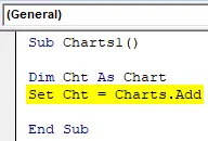
Шаг 3: Чтобы использовать графики, нам нужно вызвать метод add, как показано ниже.
Код:
Sub Charts1 () Dim Cht As Chart Set Cht = Charts.Add End Sub
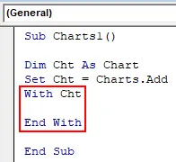
Шаг 4. Чтобы использовать свойства объекта диаграммы, вставьте оператор With в код, как показано ниже.
Код:
Sub Charts1 () Dim Cht As Chart Set Cht = Charts.Add With Cht End With End Sub
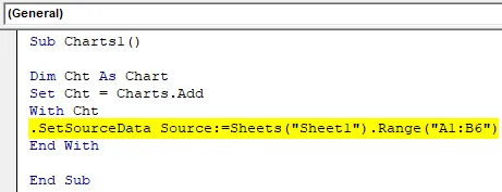
Шаг 5: Теперь давайте предоставим источник для этой диаграммы, начнем с точечного оператора, и он даст нам дополнительные возможности. Введите следующий код ниже, чтобы ввести источник для диаграммы.
Код:
Sub Charts1 () Dim Cht As Chart Set Cht = Charts.Add With Cht .SetSourceData Source: = Sheets ("Sheet1"). Range ("A1: B6") Конец с End Sub
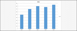
Шаг 6: Теперь запомните, что мы не предоставили никакой тип диаграммы, сначала давайте запустим приведенный выше код, нажав клавишу F5, и посмотрим, какой тип диаграммы будет вставлен.
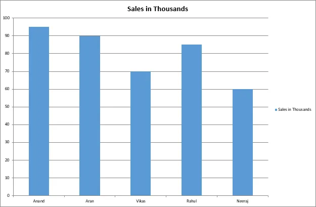
У нас есть новый лист, который называется «Диаграмма», и в нем есть наш график.
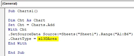
Шаг 7: Теперь давайте дадим коду тип диаграммы, которую мы хотим использовать для этого представления,
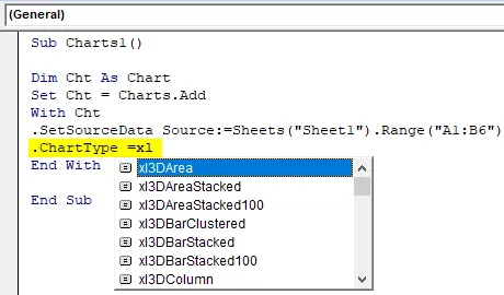
Шаг 8: Давайте выберем трехмерную область для этого примера, как показано ниже,
Код:
Sub Charts1 () Dim Cht As Chart Set Cht = Charts.Add With Cht .SetSourceData Source: = Sheets ("Sheet1"). Range ("A1: B6") .ChartType = xl3DArea End End End Sub
Шаг 9: Запустите код, нажав клавишу F5 или нажав кнопку «Воспроизвести» и проверьте тип диаграммы на рабочем листе.
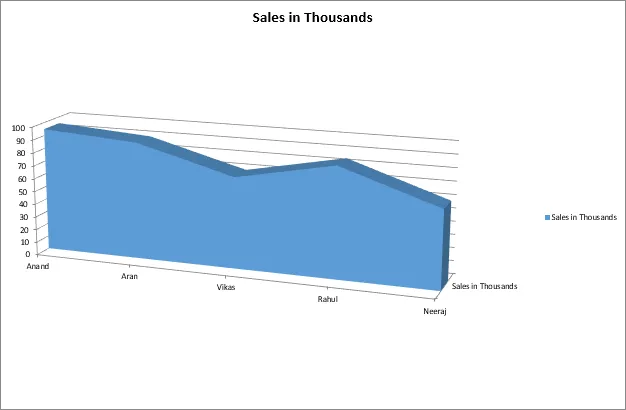
Теперь помните, что каждый раз, когда мы запускаем код, он создает новый лист диаграммы для нас. Это также называется листом диаграммы, потому что он создает диаграммы на другом листе.
Excel VBA Charts — Пример № 2
Теперь давайте создадим встроенную диаграмму, которая означает диаграмму в листе исходных данных. Для этого выполните следующие шаги, чтобы создать диаграмму в Excel VBA.
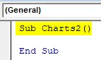
Шаг 1: В том же модуле запустите еще одну подпроцедуру следующим образом.
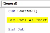
Код: Sub Charts2 () End Sub
Шаг 2: Снова объявите переменную как тип диаграммы следующим образом.
Код:
Sub Charts2 () Dim Cht1 As Chart End Sub
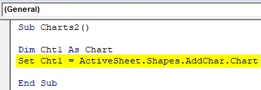
Шаг 3: Разница во встроенных диаграммах заключается в том, что мы ссылаемся на рабочий лист с данными в качестве активного листа с помощью следующего кода, показанного ниже.
Код:
Sub Charts2 () Dim Cht1 As Chart Set Cht1 = ActiveSheet.Shapes.AddChart.Chart End Sub
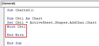
Шаг 4: Теперь остальная часть создания и проектирования диаграмм схожа, мы снова добавили оператор With в код следующим образом.
Код:
Sub Charts2 () Dim Cht1 As Chart Set Cht1 = ActiveSheet.Shapes.AddChart.Chart с Cht1, заканчивающимся End Sub
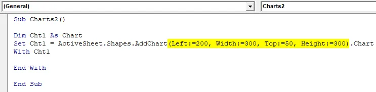
Шаг 5: Позвольте нам указать место, где будет находиться наша диаграмма, поскольку мы не хотим, чтобы она находилась над нашими данными, поэтому перед С помощью Statement добавьте следующий код туда, где мы установили нашу диаграмму, следующим образом.
Код:
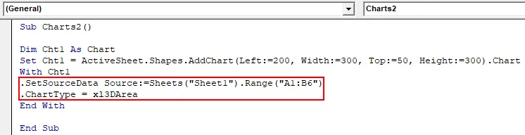
Sub Charts2 () Dim Cht1 As Chart1 Set Chart1 = ActiveSheet.Shapes.AddChart (Слева: = 200, Ширина: = 300, Верх: = 50, Высота: = 300). Диаграмма с Cht1 Конец с Концом Sub
Шаг 6: Теперь давайте предоставим источник данных и тип диаграммы, которые мы хотим видеть следующим образом.
Код:
Sub Charts2 () Dim Cht1 как набор диаграмм Cht1 = ActiveSheet.Shapes.AddChart (Слева: = 200, Ширина: = 300, Верх: = 50, Высота: = 300). Диаграмма с Cht1 .SetSourceData Source: = Sheets ("Sheet1 ") .Range (" A1: B6 ") .ChartType = xl3DArea End End End Sub
Шаг 7: Запустите код, нажав клавишу F5 или нажав кнопку «Воспроизвести» и посмотрите результат на нашем листе, где данные следующие.
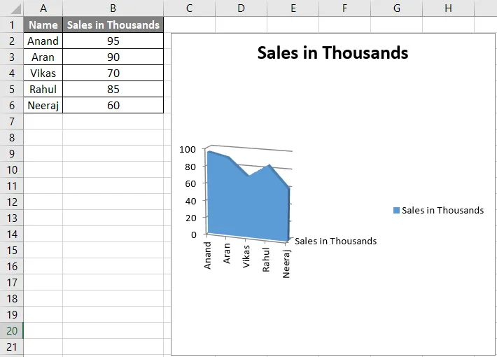
Это называется встроенной диаграммой, поскольку диаграмма находится на том же листе, что и данные.
Excel VBA Charts — Пример № 3
Существует также другой способ создания диаграмм в наших таблицах с использованием VBA. Этот метод известен как метод ChartsObject.
Шаг 1: В том же модуле давайте начнем с третьей подпроцедуры следующим образом.
Код:
Sub Charts3 () End Sub
Шаг 2: Конус как лист данных, другой тип как диапазон и один как объект диаграммы, как показано ниже.
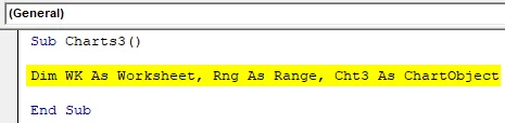
Код:
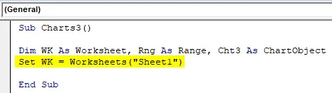
Sub Charts3 () Dim WK As Worksheet, Rng As Range, Cht3 As ChartObject End Sub
Шаг 3: Сначала установите на листе, где находятся данные, в данном случае это лист 1.
Код:
Sub Charts3 () Dim WK As Worksheet, Rng As Range, Cht3 As ChartObject Set WK = Worksheets ("Sheet1") End Sub
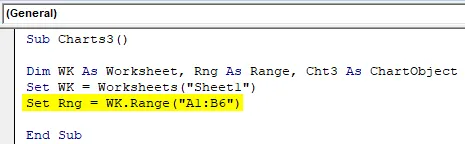
Шаг 4: Теперь выберите диапазон данных у нас следующим образом.
Код:
Sub Charts3 () Dim WK As Worksheet, Rng As Range, Cht3 As ChartObject Set WK = Worksheets ("Sheet1") Set Rng = WK.Range ("A1: B6") End Sub
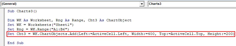
Шаг 5: Теперь установите объект диаграммы, чтобы добавить диаграмму, используя свойство объекта диаграммы следующим образом.
Код:
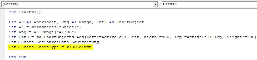
Sub Charts3 () Dim WK As Worksheet, Rng As Range, Cht3 As ChartObject Set WK = Worksheets ("Sheet1") Set Rng = WK.Range ("A1: B6") Set Cht3 = WK.ChartObjects.Add (Left: = ActiveCell.Left, ширина: = 400, верх: = ActiveCell.Top, высота: = 200) End Sub
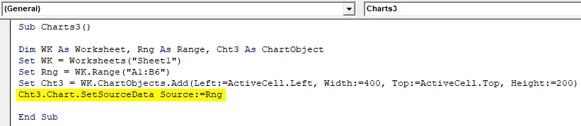
Шаг 6: Теперь давайте приведем источник диаграммы следующим образом.
Код:
Sub Charts3 () Dim WK As Worksheet, Rng As Range, Cht3 As ChartObject Set WK = Worksheets ("Sheet1") Set Rng = WK.Range ("A1: B6") Set Cht3 = WK.ChartObjects.Add (Left: = ActiveCell.Left, Width: = 400, Top: = ActiveCell.Top, Height: = 200) Cht3.Chart.SetSourceData Source: = Rng End Sub
Шаг 7: Теперь выберите желаемый тип диаграммы следующим образом.
Код:
Sub Charts3 () Dim WK As Worksheet, Rng As Range, Cht3 As ChartObject Set WK = Worksheets ("Sheet1") Set Rng = WK.Range ("A1: B6") Set Cht3 = WK.ChartObjects.Add (Left: = ActiveCell.Left, Width: = 400, Top: = ActiveCell.Top, Height: = 200) Cht3.Chart.SetSourceData Source: = Rng Cht3.Chart.ChartType = xl3DColumn End Sub
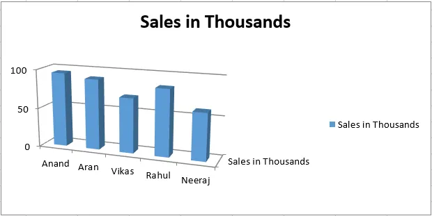
Шаг 8: Запустите код, нажав клавишу F5 или нажав кнопку «Воспроизвести» и посмотрите результат на листе 1.
То, что нужно запомнить
- Мы можем решить, какой тип диаграмм мы хотим использовать, установив тип диаграммы.
- В типе диаграммы — количество раз, когда мы запускаем код, новый лист создается под уникальным именем диаграммы с диаграммой внутри.
- Объект Chart также является членом листов, в которых есть как диаграммы, так и листы.
- Чтобы использовать объект диаграммы, нам нужно использовать инструкцию SET, чтобы сначала установить диаграмму.
Рекомендуемые статьи
Это руководство к диаграммам VBA. Здесь мы обсудим, как создавать диаграммы в Excel с использованием кода VBA, а также с практическими примерами и загружаемым шаблоном Excel. Вы также можете просмотреть наши другие предлагаемые статьи —
- VBA PowerPoint
- Комбинированные диаграммы Excel
- Проверка файла VBA существует
- Столбчатая диаграмма Excel
In this Article
- Creating an Embedded Chart Using VBA
- Specifying a Chart Type Using VBA
- Adding a Chart Title Using VBA
- Changing the Chart Background Color Using VBA
- Changing the Chart Plot Area Color Using VBA
- Adding a Legend Using VBA
- Adding Data Labels Using VBA
- Adding an X-axis and Title in VBA
- Adding a Y-axis and Title in VBA
- Changing the Number Format of An Axis
- Changing the Formatting of the Font in a Chart
- Deleting a Chart Using VBA
- Referring to the ChartObjects Collection
- Inserting a Chart on Its Own Chart Sheet
Excel charts and graphs are used to visually display data. In this tutorial, we are going to cover how to use VBA to create and manipulate charts and chart elements.
You can create embedded charts in a worksheet or charts on their own chart sheets.
Creating an Embedded Chart Using VBA
We have the range A1:B4 which contains the source data, shown below:
You can create a chart using the ChartObjects.Add method. The following code will create an embedded chart on the worksheet:
Sub CreateEmbeddedChartUsingChartObject()

Dim embeddedchart As ChartObject

Set embeddedchart = Sheets("Sheet1").ChartObjects.Add(Left:=180, Width:=300, Top:=7, Height:=200)
embeddedchart.Chart.SetSourceData Source:=Sheets("Sheet1").Range("A1:B4")

End Sub
The result is:
You can also create a chart using the Shapes.AddChart method. The following code will create an embedded chart on the worksheet:
Sub CreateEmbeddedChartUsingShapesAddChart()

Dim embeddedchart As Shape

Set embeddedchart = Sheets("Sheet1").Shapes.AddChart
embeddedchart.Chart.SetSourceData Source:=Sheets("Sheet1").Range("A1:B4")

End Sub
Specifying a Chart Type Using VBA
We have the range A1:B5 which contains the source data, shown below:
You can specify a chart type using the ChartType Property. The following code will create a pie chart on the worksheet since the ChartType Property has been set to xlPie:
Sub SpecifyAChartType()

Dim chrt As ChartObject

Set chrt = Sheets("Sheet1").ChartObjects.Add(Left:=180, Width:=270, Top:=7, Height:=210)
chrt.Chart.SetSourceData Source:=Sheets("Sheet1").Range("A1:B5")
chrt.Chart.ChartType = xlPie

End Sub
The result is:
These are some of the popular chart types that are usually specified, although there are others:
- xlArea
- xlPie
- xlLine
- xlRadar
- xlXYScatter
- xlSurface
- xlBubble
- xlBarClustered
- xlColumnClustered
Adding a Chart Title Using VBA
We have a chart selected in the worksheet as shown below:
You have to add a chart title first using the Chart.SetElement method and then specify the text of the chart title by setting the ChartTitle.Text property.
The following code shows you how to add a chart title and specify the text of the title of the Active Chart:
Sub AddingAndSettingAChartTitle()

ActiveChart.SetElement (msoElementChartTitleAboveChart)
    ActiveChart.ChartTitle.Text = "The Sales of the Product"

End Sub
The result is:
Note: You must select the chart first to make it the Active Chart to be able to use the ActiveChart object in your code.
Changing the Chart Background Color Using VBA
We have a chart selected in the worksheet as shown below:
You can change the background color of the entire chart by setting the RGB property of the FillFormat object of the ChartArea object. The following code will give the chart a light orange background color:
Sub AddingABackgroundColorToTheChartArea()

ActiveChart.ChartArea.Format.Fill.ForeColor.RGB = RGB(253, 242, 227)

End Sub
The result is:

You can also change the background color of the entire chart by setting the ColorIndex property of the Interior object of the ChartArea object. The following code will give the chart an orange background color:
Sub AddingABackgroundColorToTheChartArea()

ActiveChart.ChartArea.Interior.ColorIndex = 40

End Sub
The result is:
Note: The ColorIndex property allows you to specify a color based on a value from 1 to 56, drawn from the preset palette, to see which values represent the different colors, click here.
Changing the Chart Plot Area Color Using VBA
We have a chart selected in the worksheet as shown below:
You can change the background color of just the plot area of the chart, by setting the RGB property of the FillFormat object of the PlotArea object. The following code will give the plot area of the chart a light green background color:
Sub AddingABackgroundColorToThePlotArea()

ActiveChart.PlotArea.Format.Fill.ForeColor.RGB = RGB(208, 254, 202)

End Sub
The result is:
Adding a Legend Using VBA
We have a chart selected in the worksheet, as shown below:
You can add a legend using the Chart.SetElement method. The following code adds a legend to the left of the chart:
Sub AddingALegend()

ActiveChart.SetElement (msoElementLegendLeft)

End Sub
The result is:
You can specify the position of the legend in the following ways:
- msoElementLegendLeft – displays the legend on the left side of the chart.
- msoElementLegendLeftOverlay – overlays the legend on the left side of the chart.
- msoElementLegendRight – displays the legend on the right side of the chart.
- msoElementLegendRightOverlay – overlays the legend on the right side of the chart.
- msoElementLegendBottom – displays the legend at the bottom of the chart.
- msoElementLegendTop – displays the legend at the top of the chart.
VBA Coding Made Easy
Stop searching for VBA code online. Learn more about AutoMacro — A VBA Code Builder that allows beginners to code procedures from scratch with minimal coding knowledge and with many time-saving features for all users!

Learn More
Adding Data Labels Using VBA
We have a chart selected in the worksheet, as shown below:
You can add data labels using the Chart.SetElement method. The following code adds data labels to the inside end of the chart:
Sub AddingADataLabels()

ActiveChart.SetElement msoElementDataLabelInsideEnd

End Sub
The result is:

You can specify how the data labels are positioned in the following ways:
- msoElementDataLabelShow – display data labels.
- msoElementDataLabelRight – displays data labels on the right of the chart.
- msoElementDataLabelLeft – displays data labels on the left of the chart.
- msoElementDataLabelTop – displays data labels at the top of the chart.
- msoElementDataLabelBestFit – determines the best fit.
- msoElementDataLabelBottom – displays data labels at the bottom of the chart.
- msoElementDataLabelCallout – displays data labels as a callout.
- msoElementDataLabelCenter – displays data labels on the center.
- msoElementDataLabelInsideBase – displays data labels on the inside base.
- msoElementDataLabelOutSideEnd – displays data labels on the outside end of the chart.
- msoElementDataLabelInsideEnd – displays data labels on the inside end of the chart.
Adding an X-axis and Title in VBA
We have a chart selected in the worksheet, as shown below:
You can add an X-axis and X-axis title using the Chart.SetElement method. The following code adds an X-axis and X-axis title to the chart:
Sub AddingAnXAxisandXTitle()

With ActiveChart
.SetElement msoElementPrimaryCategoryAxisShow
.SetElement msoElementPrimaryCategoryAxisTitleHorizontal
End With


End Sub
The result is:
Adding a Y-axis and Title in VBA
We have a chart selected in the worksheet, as shown below:
You can add a Y-axis and Y-axis title using the Chart.SetElement method. The following code adds an Y-axis and Y-axis title to the chart:
Sub AddingAYAxisandYTitle()

With ActiveChart
.SetElement msoElementPrimaryValueAxisShow
.SetElement msoElementPrimaryValueAxisTitleHorizontal
End With
End Sub
The result is:
VBA Programming | Code Generator does work for you!
Changing the Number Format of An Axis
We have a chart selected in the worksheet, as shown below:
You can change the number format of an axis. The following code changes the number format of the y-axis to currency:
Sub ChangingTheNumberFormat()

ActiveChart.Axes(xlValue).TickLabels.NumberFormat = "$#,##0.00"

End Sub
The result is:
Changing the Formatting of the Font in a Chart
We have the following chart selected in the worksheet as shown below:

You can change the formatting of the entire chart font, by referring to the font object and changing its name, font weight, and size. The following code changes the type, weight and size of the font of the entire chart.
Sub ChangingTheFontFormatting()

With ActiveChart


.ChartArea.Format.TextFrame2.TextRange.Font.Name = "Times New Roman"
.ChartArea.Format.TextFrame2.TextRange.Font.Bold = True
.ChartArea.Format.TextFrame2.TextRange.Font.Size = 14

End With
The result is:
Deleting a Chart Using VBA
We have a chart selected in the worksheet, as shown below:
We can use the following code in order to delete this chart:
Sub DeletingTheChart()

ActiveChart.Parent.Delete

End Sub
Referring to the ChartObjects Collection
You can access all the embedded charts in your worksheet or workbook by referring to the ChartObjects collection. We have two charts on the same sheet shown below:
We will refer to the ChartObjects collection in order to give both charts on the worksheet the same height, width, delete the gridlines, make the background color the same, give the charts the same plot area color and make the plot area line color the same color:
Sub ReferringToAllTheChartsOnASheet()

Dim cht As ChartObject

For Each cht In ActiveSheet.ChartObjects
cht.Height = 144.85
cht.Width = 246.61

cht.Chart.Axes(xlValue).MajorGridlines.Delete
cht.Chart.PlotArea.Format.Fill.ForeColor.RGB = RGB(242, 242, 242)
cht.Chart.ChartArea.Format.Fill.ForeColor.RGB = RGB(234, 234, 234)
cht.Chart.PlotArea.Format.Line.ForeColor.RGB = RGB(18, 97, 172)

Next cht

End Sub
The result is:
Inserting a Chart on Its Own Chart Sheet
We have the range A1:B6 which contains the source data, shown below:
You can create a chart using the Charts.Add method. The following code will create a chart on its own chart sheet:
Sub InsertingAChartOnItsOwnChartSheet()

Sheets("Sheet1").Range("A1:B6").Select
Charts.Add

End Sub
The result is:
See some of our other charting tutorials:
Charts in Excel
Create a Bar Chart in VBA
Excel Chart VBA Examples and Tutorials
Excel charts are one of the awesome tools available to represent the data in rich visualized graphs. Here are the most frequently used Excel Chart VBA Examples and Tutorials. You can access chart objects, properties and dealing with the methods.
Here are the top most Excel Chart VBA Examples and Tutorials, show you how to deal with chart axis, chart titles, background colors,chart data source, chart types, series and many other chart objects.
Excel Chart VBA Examples and Tutorials – Learning Path
- Example tutorials on Creating Charts using Excel VBA:
- Example tutorials on Chart Type using Excel VBA:
- Example Tutorials on Formatting Chart Objects using Excel VBA:
- Example Tutorials on Chart Collection in Excel VBA:
- Other useful Examples and tutorials on Excel VBA Charting:
- Excel VBA Charting Constants and Enumerations:
- Example File for Free Download:
Creating Charts using Excel VBA
We can create the chart using different methods in Excel VBA, following are the various Excel Chart VBA Examples and Tutorials to show you creating charts in Excel using VBA.
1. Adding New Chart for Selected Data using Sapes.AddChart Method in Excel VBA
The following Excel Chart VBA Examples works similarly when we select some data and click on charts from Insert Menu and to create a new chart. This will create basic chart in an existing worksheet.
Sub ExAddingNewChartforSelectedData_Sapes_AddChart_Method()
Range("C5:D7").Select
ActiveSheet.Shapes.AddChart.Select
End Sub
2. Adding New Chart for Selected Data using Charts.Add Method : Creating Chart Sheet in Excel VBA
The following Excel Chart VBA Examples method will add new chart into new worksheet by default. You can specify a location to embedded in a particular worksheet.
'Here is the other method to add charts using Chart Object. It will add a new chart for the selected data as new chart sheet.
Sub ExAddingNewChartforSelectedData_Charts_Add_Method_SheetChart()
Range("C5:D7").Select
Charts.Add
End Sub
3. Adding New Chart for Selected Data using Charts.Add Method : In Existing Sheet using Excel VBA
We can use the Charts.Add method to create a chart in existing worksheet. We can specify the position and location as shown below. This will create a new chart in a specific worksheet.
Sub ExAddingNewChartforSelectedData_Charts_Add_Method_InSheet()

Range("C5:D7").Select
Charts.Add
ActiveChart.Location Where:=xlLocationAsObject, Name:="Sheet1"

End Sub
4. Difference between embedded Chart and Chart Sheet in Excel:
Both are similar except event handlers, Chart Sheets will have the event handlers,we can write event programming for Chart Sheets. And the other type embedded charts can not support the event handlers. We can write classes to handle the events for the embedded chart, but not recommended.
We have seen multiple methods to create charts, but we cant set the chart at particular position using the above codes. You can use the ChartObjects.Add method to specify the position of the chart.
5. Adding New Chart for Selected Data using ChartObjects.Add Method in Excel VBA
ChartObjects.Add method is the best method as it is very easy to play with the chart objects to change the settings.
Sub ExAddingNewChartforSelectedData_ChartObjects_Add_Method()
With ActiveSheet.ChartObjects.Add(Left:=300, Width:=300, Top:=10, Height:=300)
.Chart.SetSourceData Source:=Sheets("Temp").Range("C5:D7")
End With
End Sub
6. Assigning Charts to an Object in Excel VBA
Here is another Excel Chart VBA Examples with ChartObjects, here we will assign to an Object and play with that.
Sub ExAddingNewChartforSelectedData_ChartObjects_Object()
Dim cht As Object
Set cht = ActiveSheet.ChartObjects.Add(Left:=300, Width:=300, Top:=10, Height:=300)
cht.Chart.SetSourceData Source:=Sheets("Temp").Range("C5:D7")
End Sub
7. Changing the Chart Position in Excel VBA
The following VBA example will show you how to change the chart position.
Sub ExAddingNewChartforSelectedData_Object_Position()
Dim cht As Object
Set cht = ActiveSheet.ChartObjects.Add(Left:=300, Width:=300, Top:=10, Height:=300)
cht.Chart.SetSourceData Source:=Sheets("Temp").Range("C5:D7")
cht.Left = 350
cht.Width = 400
cht.Top = 30
cht.Height = 200
End Sub
8. Align Chart Object at a Particular Range or Cell in Excel VBA
You can set the top,left, height and width properties of a chart object to align in a particular position.
Sub AlignChartAtParticularRange()
' Chart Align

With ActiveSheet.ChartObjects(1)
.Left = Range("A6").Left
.Top = Range("A7").Top
.Width = Range("D6").Left
.Height = Range("D16").Top - Range("D6").Top
End With

End Sub
9. Use with statement while dealing with Charts and avoid the accessing the same object repeatedly in Excel VBA
If you are dealing with the same object, it is better to use with statement. It will make the program more clear to understand and executes faster.
Sub ExChartPostion_Object_Position()
Dim cht As Object
Set cht = ActiveSheet.ChartObjects.Add(Left:=300, Width:=300, Top:=10, Height:=300)
With cht
.Chart.SetSourceData Source:=Sheets("Temp").Range("C5:D7")
.Left = 350
.Width = 400
.Top = 30
.Height = 200
End With
End Sub
10. You can use ActiveChart Object to access the active chart in Excel VBA
Active chart is the chart which is currently selected or activated in your active sheet.
Sub ExChartPostion_ActiveChart()
ActiveSheet.ChartObjects.Add(Left:=300, Width:=300, Top:=10, Height:=300).Activate
With ActiveChart
.SetSourceData Source:=Sheets("Temp").Range("C5:D7")
.Parent.Left = 350
.Parent.Width = 400
.Parent.Top = 30
.Parent.Height = 200
End With
End Sub
Top
Setting Chart Types using Excel VBA
We have verity of chart in Excel, we can use VBA to change and set the suitable chart type based on the data which we want to present. Below are the Excel Chart VBA Examples and Tutorials to change the chart type.
We can use Chart.Type property to set the chart type, here we can pass Excel chart constants or chart enumerations to set the chart type. Please refer the following table to understand the excel constants and enumerations.
11. Example to Change Chart type using Excel Chart Enumerations in Excel VBA
This Excel Chart VBA Example will use 1 as excel enumeration to plot the Aria Chart. Please check here list of enumerations available for Excel VBA Charting
Sub Ex_ChartType_Enumeration()
Dim cht As Object
Set cht = ActiveSheet.ChartObjects.Add(Left:=300, Width:=300, Top:=10, Height:=300)
With cht
.Chart.SetSourceData Source:=Sheets("Temp").Range("C5:D7")
.Chart.Type = 1 ' for aria chart
End With
End Sub
12. Example to Change Chart type using Excel Chart Constants in VBA
This Excel Chart VBA Example will use xlArea as excel constant to plot the Aria Chart. Please check here for list of enumerations available in Excel VBA Charting
Sub Ex_ChartType_xlConstant()
Dim cht As Object
Set cht = ActiveSheet.ChartObjects.Add(Left:=300, Width:=300, Top:=10, Height:=300)
With cht
.Chart.SetSourceData Source:=Sheets("Temp").Range("C5:D7")
.Chart.Type = xlArea
End With
End Sub
xlConstants is recommended than Excel Enumeration, as it is easy to understand and remember. Following are frequently used chart type examples:
13. Example to set the type as a Pie Chart in Excel VBA
The following VBA code using xlPie constant to plot the Pie chart. Please check here for list of enumerations available in Excel VBA Charting
Sub Ex_ChartType_Pie_Chart()
Dim cht As Object
Set cht = ActiveSheet.ChartObjects.Add(Left:=300, Width:=300, Top:=10, Height:=300)
With cht
.Chart.SetSourceData Source:=Sheets("Temp").Range("C5:D7")
.Chart.Type = xlPie
End With
End Sub
14. Example to set the chart type as a Line Chart in Excel VBA
The following VBA code using xlLine constant to plot the Pie chart. Please check here for list of enumerations available in Excel VBA Charting
Sub Ex_ChartType_Line_Chart()
Dim cht As Object
Set cht = ActiveSheet.ChartObjects.Add(Left:=300, Width:=300, Top:=10, Height:=300)
With cht
.Chart.SetSourceData Source:=Sheets("Temp").Range("C5:D7")
.Chart.Type = xlLine
End With
End Sub
15. Example to set the chart type as a Bar Chart in Excel VBA
The following VBA code using xlBar constant to plot the Pie chart. Please check here for list of enumerations available in Excel VBA Charting
Sub Ex_ChartType_Bar_Chart()
Dim cht As Object
Set cht = ActiveSheet.ChartObjects.Add(Left:=300, Width:=300, Top:=10, Height:=300)
With cht
.Chart.SetSourceData Source:=Sheets("Temp").Range("C5:D7")
.Chart.Type = xlBar
End With
End Sub
16. Example to set the chart type as a XYScatter Chart in Excel VBA
The following code using xlXYScatter constant to plot the Pie chart. Please check here for list of enumerations available in Excel VBA Charting
Sub Ex_ChartType_XYScatter_Chart()
Dim cht As Object
Set cht = ActiveSheet.ChartObjects.Add(Left:=300, Width:=300, Top:=10, Height:=300)
With cht
.Chart.SetSourceData Source:=Sheets("Temp").Range("C5:D7")
.Chart.Type = xlXYScatter
End With
End Sub
Here is the complete list of Excel Chart Types, Chart Enumerations and Chart Constants:
Top
Formatting Chart Objects using Excel VBA
Below are Excel Chart VBA Examples to show you how to change background colors of charts, series and changing the different properties of charts like Chart Legends, Line Styles, Number Formatting. You can also find the examples on Chart Axis and Chart Axes Setting and Number Formats.
17. Changing Chart Background Color – Chart Aria Interior Color in Excel VBA
The following VBA code will change the background color of the Excel Chart.
Sub Ex_ChartAriaInteriorColor()
Dim cht As Object
Set cht = ActiveSheet.ChartObjects.Add(Left:=300, Width:=300, Top:=10, Height:=300)
With cht
.Chart.SetSourceData Source:=Sheets("Temp").Range("C5:D7")
.Chart.ChartArea.Interior.ColorIndex = 3
End With
End Sub
18. Changing PlotAria Background Color – PlotAria Interior Color in Excel VBA
The following code will change the background color of Plot Area in Excel VBA.
Sub Ex_PlotAriaInteriorColor()
Dim cht As Object
Set cht = ActiveSheet.ChartObjects.Add(Left:=300, Width:=300, Top:=10, Height:=300)
With cht
.Chart.SetSourceData Source:=Sheets("Temp").Range("C5:D7")
.Chart.PlotArea.Interior.ColorIndex = 5
End With
End Sub
19.Changing Chart Series Background Color – Series Interior Color in Excel VBA
The following code is for changing the background color of a series using Excel VBA.
Sub Ex_SeriesInteriorColor()
Dim cht As Object
Set cht = ActiveSheet.ChartObjects.Add(Left:=300, Width:=300, Top:=10, Height:=300)
With cht
.Chart.SetSourceData Source:=Sheets("Temp").Range("C5:D7")
.Chart.SeriesCollection(1).Format.Fill.ForeColor.RGB = rgbRed
.Chart.SeriesCollection(2).Interior.ColorIndex = 5

End With
End Sub
20. Changing Chart Series Marker Style in Excel VBA
Here is the code to change the series marker style using Excel VBA, you can change to circle, diamond, square,etc. Check the excel constants and enumerations for more options available in excel vba.
Sub Ex_ChangingMarkerStyle()
Dim cht As Object
Set cht = ActiveSheet.ChartObjects.Add(Left:=300, Width:=300, Top:=10, Height:=300)
With cht
.Chart.SetSourceData Source:=Sheets("Temp").Range("C5:D7")
.Chart.Type = xlLine
.Chart.SeriesCollection(1).MarkerStyle = 7
End With
End Sub
21. Changing Chart Series Line Style in Excel VBA
Here is the code to change the line color using Excel VBA, it will change the line style from solid to dash. Check the excel constants for more options.
Sub Ex_ChangingLineStyle()
Dim cht As Object
Set cht = ActiveSheet.ChartObjects.Add(Left:=300, Width:=300, Top:=10, Height:=300)
With cht
.Chart.SetSourceData Source:=Sheets("Temp").Range("C5:D7")
.Chart.Type = xlLine
.Chart.SeriesCollection(1).Border.LineStyle = xlDash
End With
End Sub
22. Changing Chart Series Border Color in Excel VBA
Here is the code for changing series borders in Excel VBA.
Sub Ex_ChangingBorderColor()
Dim cht As Object
Set cht = ActiveSheet.ChartObjects.Add(Left:=300, Width:=300, Top:=10, Height:=300)
With cht
.Chart.SetSourceData Source:=Sheets("Temp").Range("C5:D7")
.Chart.Type = xlBar
.Chart.SeriesCollection(1).Border.ColorIndex = 3
End With
End Sub
23. Change Chart Axis NumberFormat in Excel VBA
This code will change the chart axis number format using excel vba.
Sub Ex_ChangeAxisNumberFormat()
Dim cht As Object
Set cht = ActiveSheet.ChartObjects.Add(Left:=300, Width:=300, Top:=10, Height:=300)
With cht
.Chart.SetSourceData Source:=Sheets("Temp").Range("C5:D7")
.Chart.Type = xlLine
.Chart.Axes(xlValue).TickLabels.NumberFormat = "0.00"
End With
End Sub
24. Formatting Axis Labels: Changing Axis Font to Bold using Excel VBA
The following example is for formating Axis labels using Excel VBA.
Sub Ex_ChangeAxisFormatFontBold()
Dim cht As Object
Set cht = ActiveSheet.ChartObjects.Add(Left:=300, Width:=300, Top:=10, Height:=300)
With cht
.Chart.SetSourceData Source:=Sheets("Temp").Range("C5:D7")
.Chart.Type = xlLine
.Chart.Axes(xlCategory).TickLabels.Font.FontStyle = "Bold"
End With
End Sub
25. Two Y-axes Left and Right of Charts(Primary Axis and Secondary Axis) using Excel VBA
This code will set the series 2 into secondary Axis using Excel VBA.
Sub Ex_ChangeAxistoSecondary()
Dim cht As Object
Set cht = ActiveSheet.ChartObjects.Add(Left:=300, Width:=300, Top:=10, Height:=300)
With cht
.Chart.SetSourceData Source:=Sheets("Temp").Range("C5:D7")
.Chart.Type = xlLine
.Chart.SeriesCollection(2).AxisGroup = 2
End With
End Sub
Top
Chart Collection in Excel VBA
You can use ChartObject Collection to loop through the all charts in worksheet or workbook using Excel VBA. And do whatever you want to do with that particular chart. Here are Excel Chart VBA Examples to deal with Charts using VBA.
26. Set equal widths and heights for all charts available in a Worksheet using Excel VBA
Following is the Excel VBA code to change the chart width and height.
Sub Ex_ChartCollections_Change_widths_heights()
Dim cht As Object
For Each cht In ActiveSheet.ChartObjects
cht.Width = 400
cht.Height = 200
Next

End Sub
27. Delete All Charts in a Worksheet using Excel VBA
Following is the Excel VBA example to delete all charts in worksheet.
Sub Ex_DeleteAllCharts()
Dim cht As Object
For Each cht In ActiveSheet.ChartObjects
cht.Delete
Next

End Sub
Top
Other useful Examples and tutorials on Excel VBA Charting
28. Set Chart Data Source using Excel VBA
Below is the Excel Chart VBA Example to set the chart data source. You can set it by using .SetSourceData Source property of a chart
Sub Ex_ChartDataSource()

Dim cht As Chart

'Add new chart
ActiveSheet.Shapes.AddChart.Select
With ActiveChart
'Specify source data and orientation
.SetSourceData Source:=Sheet1.Range("A1:C5")
End With

End Sub
29. Swap or Switch Rows and Columns in Excel Charts using VBA
Here is the excel VBA code to swap the Rows to Columns.
Sub Ex_SwitchRowsColumns()

Dim cht As Chart

'Add new chart
ActiveSheet.Shapes.AddChart.Select
With ActiveChart
'Specify source data and orientation
.SetSourceData Source:=Sheets("Temp").Range("C5:D7"), PlotBy:=xlRows ' you can use xlColumns to swith it
End With

End Sub
30. Set Chart Data Labels and Legends using Excel VBA
You can set Chart Data Labels and Legends by using SetElement property in Excl VBA
Sub Ex_AddDataLabels()

Dim cht As Chart

'Add new chart
ActiveSheet.Shapes.AddChart.Select
With ActiveChart
'Specify source data and orientation
.SetSourceData Source:=Sheet1.Range("A1:B5"), PlotBy:=xlColumns
'Set Chart type
.ChartType = xlPie
'set data label at center
.SetElement (msoElementDataLabelCenter)
'set legend at bottom
.SetElement (msoElementLegendBottom)
End With
End Sub
31. Changing Axis Titles of a Chart in Excel VBA
Following is the code to change the chart Axis titles using Excel VBA..
Sub Ex_ChangeAxisTitles()
activechart.chartobjects(1).activate
ActiveChart.Axes(xlCategory).HasTitle = True
ActiveChart.Axes(xlCategory).AxisTitle.Text = "Quarter"

ActiveChart.Axes(xlValue).HasTitle = True
ActiveChart.Axes(xlValue).AxisTitle.Text = "Sales"

End Sub
32. Change Titles of a Chart using Excel VBA
Following is the code to change the chart titles using Excel VBA..
Sub Ex_ChangeChartTitles()
ActiveSheet.ChartObjects(1).Activate
ActiveChart.HasTitle = True
ActiveChart.ChartTitle.Text = "Overal Summary"

End Sub
33. Send an Excel Chart to an Outlook email using VBA
Download Example File:
ANALYSIS TABS – SendExcelChartToOutLook.xlsm
Following is the code to Send an Excel Chart to an Outlook email using VBA.
Sub SendChartThroughMail()
'Add refernce to Microsoft Outlook object Library

Dim olMail As MailItem
Dim objOL As Object
Dim sImgPath As String

Dim sHi As String
Dim sBody As String
Dim sThanks As String

' Saving chart as image
sImgPath = ThisWorkbook.Path & "Temp_" & Format(Now(), "DD_MM_YY_HH_MM_SS") & ".bmp"
Sheets("Sheet1").ChartObjects(1).Chart.Export sImgPath

'creating html body with image
sHi = "<font size='3' color='black'>" & "Hi," & "<br> <br>" & "Here is the required solution: " & "<br> <br> </font>"

sBody = "<p align='Left'><img src=""cid:" & Mid(sImgPath, InStrRev(sImgPath, "") + 1) & """ width=400 height=300 > <br> <br>"

sThanks = "<font size='3'>" & "Many thanks - ANALYSISTABS.COM <br>The Complete Reference For Analyst <br> website:<A HREF=""https://www.analysistabs.com""> analysistabs.com</A>" & "<br> <br> </font>"

'sending the email

Set objOL = CreateObject("Outlook.Application")
Set olMail = objOL.CreateItem(olMailItem)

With olMail
.To = "youremail@orgdomain.com"
.Subject = "ANALYSISTABS.COM: Test Mail with chart"
.Attachments.Add sImgPath
.HTMLBody = sHi & sBody & sThanks
.Display
End With

'Delete the saved chart
Kill sImgPath

'Free-up the objects
Set olMail = Nothing
Set olApp = Nothing

End Sub
Top
Excel VBA Chart Constants and Enumerations
Chart Types, Constants and Enumerations
| CHART TYPE | VBA CONSTANT | VALUE |
|
AREA Charts |
||
| AREA | xlArea | 1 |
| STACKED AREA | xlAreaStacked | 76 |
| 100% STACKED AREA | xlAreaStacked100 | 77 |
| 3D AREA | xl3DArea | -4098 |
| 3D STACKED AREA | xl3DAreaStacked | 78 |
| 3D 100% STACKED AREA | xl3DAreaStacked100 | 79 |
|
BAR Charts |
||
| 3D CLUSTERED BAR | xl3DBarClustered | 60 |
| 3D STACKED BAR | xl3DBarStacked | 61 |
| 3D 100% STACKED BAR | xl3DBarStacked100 | 62 |
| CLUSTERED BAR | xlBarClustered | 57 |
| STACKED BAR | xlBarStacked | 58 |
| 100% STACKED BAR | xlBarStacked100 | 59 |
| CLUSTERED CONE BAR | xlConeBarClustered | 102 |
| STACKED CONE BAR | xlConeBarStacked | 103 |
| 100% STACKED CONE BAR | xlConeBarStacked100 | 104 |
| CLUSTERED CYLINDER BAR | xlCylinderBarClustered | 95 |
| STACKED CYLINDER BAR | xlCylinderBarStacked | 96 |
| 100% STACKED CYLINDER BAR | xlCylinderBarStacked100 | 97 |
| CLUSTERED PYRAMID BAR | xlPyramidBarClustered | 109 |
| STACKED PYRAMID BAR | xlPyramidBarStacked | 110 |
| 100% STACKED PYRAMID BAR | xlPyramidBarStacked100 | 111 |
| BUBBLE Charts | ||
| 3D BUBBLE, BUBBLE WITH 3D EFFECTS | xlBubble3DEffect | 87 |
| BUBBLE | xlBubble | 15 |
|
COLUMN Charts |
||
| 3D CLUSTERED COLUMN | xl3DColumnClustered | 54 |
| 3D COLUMN | xl3DColumn | -4100 |
| 3D CONE COLUMN | xlConeCol | 105 |
| 3D CYLINDER COLUMN | xlCylinderCol | 98 |
| 3D PYRAMID COLUMN | xlPyramidCol | 112 |
| 3D STACKED COLUMN | xl3DColumnStacked | 55 |
| 3D 100% STACKED COLUMN | xl3DColumnStacked100 | 56 |
| CLUSTERED COLUMN | xlColumnClustered | 51 |
| STACKED COLUMN | xlColumnStacked | 52 |
| 100% STACKED COLUMN | xlColumnStacked100 | 53 |
| CLUSTERED CONE COLUMN | xlConeColClustered | 99 |
| STACKED CONE COLUMN | xlConeColStacked | 100 |
| 100% STACKED CONE COLUMN | xlConeColStacked100 | 101 |
| CLUSTERED CYLINDER COLUMN | xlCylinderColClustered | 92 |
| STACKED CYLINDER COLUMN | xlCylinderColStacked | 93 |
| 100% STACKED CYLINDER COLUMN | xlCylinderColStacked100 | 94 |
| CLUSTERED PYRAMID COLUMN | xlPyramidColClustered | 106 |
| STACKED PYRAMID COLUMN | xlPyramidColStacked | 107 |
| 100% STACKED PYRAMID COLUMN | xlPyramidColStacked100 | 108 |
|
DOUGHNUT Charts |
||
| DOUGHNUT | xlDoughnut | -4120 |
| EXPLODED DOUGHNUT | xlDoughnutExploded | 80 |
|
LINE Charts |
||
| 3D LINE | xl3DLine | -4101 |
| LINE | xlLine | 4 |
| LINE WITH MARKERS | xlLineMarkers | 65 |
| STACKED LINE | xlLineStacked | 63 |
| 100% STACKED LINE | xlLineStacked100 | 64 |
| STACKED LINE WITH MARKERS | xlLineMarkersStacked | 66 |
| 100% STACKED LINE WITH MARKERS | xlLineMarkersStacked100 | 67 |
|
PIE Charts |
||
| 3D PIE | xl3DPie | -4102 |
| 3D EXPLODED PIE | xl3DPieExploded | 70 |
| BAR OF PIE | xlBarOfPie | 71 |
| EXPLODED PIE | xlPieExploded | 69 |
| PIE | xlPie | 5 |
| PIE OF PIE | xlPieOfPie | 68 |
|
RADAR Charts |
||
| RADAR | xlRadar | -4151 |
| FILLED RADAR | xlRadarFilled | 82 |
| RADAR WITH DATA MARKERS | xlRadarMarkers | 81 |
|
SCATTER Charts |
||
| SCATTER | xlXYScatter | -4169 |
| SCATTER WITH LINES | xlXYScatterLines | 74 |
| SCATTER WITH LINES AND NO DATA MARKERS | xlXYScatterLinesNoMarkers | 75 |
| SCATTER WITH SMOOTH LINES | xlXYScatterSmooth | 72 |
| SCATTER WITH SMOOTH LINES AND NO DATA MARKERS | xlXYScatterSmoothNoMarkers | 73 |
|
STOCK Charts |
||
| STOCK HLC (HIGH-LOW-CLOSE) | xlStockHLC | 88 |
| STOCK OHLC (OPEN-HIGH-LOW-CLOSE) | xlStockOHLC | 89 |
| STOCK VHLC (VOLUME-HIGH-LOW-CLOSE) | xlStockVHLC | 90 |
| STOCK VOHLC (VOLUME-OPEN-HIGH-LOW-CLOSE) | xlStockVOHLC | 91 |
|
SURFACE Charts |
||
| 3D SURFACE | xlSurface | 83 |
| 3D SURFACE WIREFRAME | xlSurfaceWireframe | 84 |
| SURFACE TOP VIEW | xlSurfaceTopView | 85 |
| SURFACE TOP VIEW WIREFRAME | xlSurfaceTopViewWireframe | 86 |
Marker Styles, Constants and Enumerations
| Marker Styles | Name | Value |
| Automatic markers | xlMarkerStyleAutomatic | -4105 |
| Circular markers | xlMarkerStyleCircle | 8 |
| Long bar markers | xlMarkerStyleDash | -4115 |
| Diamond-shaped markers | xlMarkerStyleDiamond | 2 |
| Short bar markers | xlMarkerStyleDot | -4118 |
| No markers | xlMarkerStyleNone | -4142 |
| Picture markers | xlMarkerStylePicture | -4147 |
| Square markers with a plus sign | xlMarkerStylePlus | 9 |
| Square markers | xlMarkerStyleSquare | 1 |
| Square markers with an asterisk | xlMarkerStyleStar | 5 |
| Triangular markers | xlMarkerStyleTriangle | 3 |
| Square markers with an X | xlMarkerStyleX | -4168 |
Line Styles, Constants and Enumerations
| Line Style | Value |
| xlContinuous | 1 |
| xlDash | -4115 |
| xlDashDot | 4 |
| xlDashDotDot | 5 |
| xlDot | -4118 |
| xlDouble | -4119 |
| xlLineStyleNone | -4142 |
| xlSlantDashDot | 13 |
Example file to Download
You can download the example file and have a look into the working codes.
ANALYSISTABS- Chart VBA Examples
Reference:
MSDN
A Powerful & Multi-purpose Templates for project management. Now seamlessly manage your projects, tasks, meetings, presentations, teams, customers, stakeholders and time. This page describes all the amazing new features and options that come with our premium templates.
Save Up to 85% LIMITED TIME OFFER

All-in-One Pack
120+ Project Management Templates
Essential Pack
50+ Project Management Templates
Excel Pack
50+ Excel PM Templates
PowerPoint Pack
50+ Excel PM Templates
MS Word Pack
25+ Word PM Templates
Ultimate Project Management Template
Ultimate Resource Management Template
Project Portfolio Management Templates
Related Posts
-
- Excel Chart VBA Examples and Tutorials – Learning Path
- Creating Charts using Excel VBA
- 1. Adding New Chart for Selected Data using Sapes.AddChart Method in Excel VBA
- 2. Adding New Chart for Selected Data using Charts.Add Method : Creating Chart Sheet in Excel VBA
- 3. Adding New Chart for Selected Data using Charts.Add Method : In Existing Sheet using Excel VBA
- 4. Difference between embedded Chart and Chart Sheet in Excel:
- 5. Adding New Chart for Selected Data using ChartObjects.Add Method in Excel VBA
- 6. Assigning Charts to an Object in Excel VBA
- 7. Changing the Chart Position in Excel VBA
- 8. Align Chart Object at a Particular Range or Cell in Excel VBA
- 9. Use with statement while dealing with Charts and avoid the accessing the same object repeatedly in Excel VBA
- 10. You can use ActiveChart Object to access the active chart in Excel VBA
- Setting Chart Types using Excel VBA
- 11. Example to Change Chart type using Excel Chart Enumerations in Excel VBA
- 12. Example to Change Chart type using Excel Chart Constants in VBA
- 13. Example to set the type as a Pie Chart in Excel VBA
- 14. Example to set the chart type as a Line Chart in Excel VBA
- 15. Example to set the chart type as a Bar Chart in Excel VBA
- 16. Example to set the chart type as a XYScatter Chart in Excel VBA
- Formatting Chart Objects using Excel VBA
- 17. Changing Chart Background Color – Chart Aria Interior Color in Excel VBA
- 18. Changing PlotAria Background Color – PlotAria Interior Color in Excel VBA
- 19.Changing Chart Series Background Color – Series Interior Color in Excel VBA
- 20. Changing Chart Series Marker Style in Excel VBA
- 21. Changing Chart Series Line Style in Excel VBA
- 22. Changing Chart Series Border Color in Excel VBA
- 23. Change Chart Axis NumberFormat in Excel VBA
- 24. Formatting Axis Labels: Changing Axis Font to Bold using Excel VBA
- 25. Two Y-axes Left and Right of Charts(Primary Axis and Secondary Axis) using Excel VBA
- Chart Collection in Excel VBA
- 26. Set equal widths and heights for all charts available in a Worksheet using Excel VBA
- 27. Delete All Charts in a Worksheet using Excel VBA
- Other useful Examples and tutorials on Excel VBA Charting
- 28. Set Chart Data Source using Excel VBA
- 29. Swap or Switch Rows and Columns in Excel Charts using VBA
- 30. Set Chart Data Labels and Legends using Excel VBA
- 31. Changing Axis Titles of a Chart in Excel VBA
- 32. Change Titles of a Chart using Excel VBA
- 33. Send an Excel Chart to an Outlook email using VBA
- Excel VBA Chart Constants and Enumerations
- Chart Types, Constants and Enumerations
- Marker Styles, Constants and Enumerations
- Line Styles, Constants and Enumerations
- Example file to Download
VBA Reference
Effortlessly
Manage Your Projects
120+ Project Management Templates
Seamlessly manage your projects with our powerful & multi-purpose templates for project management.
120+ PM Templates Includes:
30 Comments
-
Tim
December 18, 2013 at 11:33 PM — ReplyHI there PNRao,
This is a really great reference – in the past, I’ve beat around the object browser as well. I use MS Graph in an MS Access application (currently A2007 in process of being upgraded from A2003). I have numerous controls to do some of the tasks you’ve identified here and others as well. I also have a button for the very few advanced users UI have to be able to actually open MS Graph in a separate window and do formatting there. What I’m trying to figure out how to do is enumerate through ALL properties of a chart and save them as an array or tab delimited string in a database (Oracle in this case) field.
Is there anyway to do this? I’ve done lots of the sorts of enumeration that you show show excellently here. What I would very much like to do is to be able to enumerate all formatting properties of a chart to be able to store it (above) and retrieve.
Do you have any ideas? Thanks in advance,
—
Tim -
PNRao
December 19, 2013 at 11:30 AM — ReplyHi Tim,
It is good idea to store all properties as enumerations in a field and draw the charts based on the requirement. You can consider the following things to save in the data base.
1. Chart Type
2. Data Source
3. Axes (Primary/Secondary)
4. Border
5. Number Format
6. Legend Alignment
7. Data Labels
8. Chart titleYou can make all the above properties as dynamic and the other things like Colors and minimum and maximum axis should be automatic.
And you can provide UI to format the charts using drop-down lists and Text boxes. For example, you can show different chart types in drop-down and chart type can be changed based on the user selection. You can provide text box to enter the chart title, it should save in your database for chart titles enumeration to reflect on your chart.
Hope this helps, let me know if you need any help on this.
Thanks
PNRao! -
kamran
February 28, 2014 at 3:44 PM — ReplyOne of the best Tutorial for VBA macro.
-
Antoni
April 23, 2014 at 9:02 PM — ReplyHi,
My boss has asked me to do many graphics chars, i love the example and explanations that have left at this web, I would like to do what our friend says PNRao, please have you any example of how to do it?
Thank you very much.
Antoni. -
PNRao
April 24, 2014 at 8:48 PM — ReplyHi Antoni,
We can automate charting using VBA. We have provided some examples in download page. You can download and see the examples, let us know if you need any help.
Thanks-PNRao!
-
Antoni
April 25, 2014 at 8:15 PM — ReplyHi PNRao,
I can’t found examples in the Download section, can you help me please?, or can you send me a links?
Thank you.
-
PNRao
April 26, 2014 at 12:08 AM — ReplyHi Antoni,
I have added the example file at end of the post. Please download and see the code.Thanks-PNRao!
-
Sam
May 4, 2014 at 9:32 AM — ReplyHi,
I am having a task, in which i need to copy chart from one excel sheet to another excel sheet.
So can you please help me in this.
Thanks,
Sam -
PNRao
May 4, 2014 at 11:40 AM — ReplyHi Sam,
You can use the Copy method as shown below:
[vb]
Sub sbVBA_Chart_Copy()
Sheet1.ChartObjects(«Chart 1»).Copy ‘Sheet name and Chart Object name to be copied
Sheet2.Activate ‘Activate your destination Sheet
Range(«G1»).Select ‘Select your destination cell
ActiveSheet.Paste ‘Now Paste
End Sub
[/vb]Thanks-PNRao!
-
Ross
December 29, 2014 at 9:02 PM — ReplyHi PNRao,
Thanks for the above it’s really helpful, although I’m still stuck!
Is there a way to so that when making a graph it has a certain destination within the sheet so it’s not pasted over my data?
Thank you!!
-
เสื้อคู่
May 25, 2015 at 3:43 PM — ReplyHi, this weekend is pleasant in favor of me, since this moment i am reading
this great informative post here at my residence. -
Nkhoma Kenneth
October 4, 2015 at 1:27 PM — ReplyThanks very much for the tutorial, it is a great one indeed and very helpful.
Thanks to you, i have learn’t something.
-
Richard
December 1, 2015 at 4:59 PM — ReplyHi Guys
Great info – ThanksI’m trying to automate some graph formatting, and whilst I’ve worked out how to change the range for a xlTimeScale based graph, I want an easy way for the user to define which graphs need to be scaled to current month rather than all year.
I thought of putting a text string into the Alt Text Description box (found under / but how do I read that field from a macro?
If it were a shape I could use something like shapeDesc = sheet(1).Shapes(1).AlternativeText but that doesn’t work for ChartObjects.
Any ideas?
Thanks
RichardAlways learning …

-
Richard
December 1, 2015 at 7:44 PM — ReplyHah! Got it guys.
I’ve decided to scroll through each sheet. In each sheet scroll through each Shape. If the Shape.Type = msoChart Then I can pick up the Alternative Text and act accordingly.Code extract:
For lShtCtr = 1 To ThisWorkbook.Sheets.Count
Debug.Print “Checking worksheet ” & lShtCtr & ” ” & Sheets(lShtCtr).Name & “. Detected ” & ThisWorkbook.Sheets(lShtCtr).Shapes.Count & ” shapes.”
For lShapeCtr = 1 To ThisWorkbook.Sheets(lShtCtr).Shapes.Count
If ThisWorkbook.Sheets(lShtCtr).Shapes(lShapeCtr).Type = msoChart Then
myText = ThisWorkbook.Sheets(lShtCtr).Shapes(lShapeCtr).AlternativeText
Debug.Print “Alt Text in ” & ThisWorkbook.Sheets(lShtCtr).Shapes(lShapeCtr).Name & ” =:” & myText
If InStr(1, myText, “#AutoScale”, vbTextCompare) > 0 Then
Debug.Print “Scaling axes on ” & ThisWorkbook.Sheets(lShtCtr).Shapes(lShapeCtr).Name
Call ScaleAxes(ThisWorkbook.Sheets(lShtCtr), ThisWorkbook.Sheets(lShtCtr).Shapes(lShapeCtr).Name)
End If ‘myText contains #AutoScale
End If ‘Shape.Type = msoChart
Next lShapeCtr
Next lShtCtrThe debug.print allow you to see what is going on. I’ve used the magic key phrase ‘#AutoScale’ as my command
Thanks
RichardAlways learning
-
Krishnaprasad Menon
January 2, 2016 at 10:45 AM — ReplyVery nice tutorial.. Chart creating example file is not available on download… Kindly make it available
-
PNRao
January 2, 2016 at 11:38 PM — ReplyThanks for your valuable feedback and reporting an issue, we have fixed it.
Thanks-PNRao!
-
HS
March 19, 2016 at 5:12 PM — ReplyVery quickly this site will be famous amid all blogging and site-building
users, due to it’s good posts -
chris
May 9, 2016 at 1:05 AM — Replyi want to explode on a pie chart the piece with the max value. How can i do this? Also what if I have on a pie two pieces with the same max value? Thank you.
-
Nagaraju
July 1, 2016 at 12:17 PM — ReplyHi All,
I’m trying to open website through Vba code….It was done…I need small information that if need code how to search search any information in google and display.
Regards,
Nagu -
Salty
August 25, 2016 at 11:12 PM — ReplyHi
This comment relates to your Example 13, above, but may apply to all of the Chart.Type examples.
Using Excel 2016 on Windows 8, I had to change one line as follows:
From > Chart.Type = xlPie
To > Chart.Chart.Type = xlPie -
Salty
August 29, 2016 at 9:01 AM — ReplyHi
Sorry, I sent you a typo in my August 25 2016 comment. It should have said:
It should have said
To > Chart.ChartType = xlPie -
Raspreet Singh Jaggi
October 21, 2016 at 3:22 PM — ReplyYour codes are very much helpful Mr.PNRao.
-
Dwayne
November 29, 2016 at 10:01 AM — ReplyHi all,
That was quite a read! I’ve come away with many ideas for future spreadsheets..I do have one quick query, I’m using the following script to change the data range for a chart I’m using;
Sub RECPLINE()
ActiveSheet.ChartObjects(“Chart 1”).Activate
ActiveChart.SeriesCollection(1).Select
ActiveChart.SetSourceData Source:=Range(“=Data!$AR$3:$AW$31”)
End SubInstead of having 6 charts crammed into one screen, I aim to have one chart and 6 buttons to change the data range in the chart.
Everything works fine, but I have formatted the visual aspects of the chart to be more appealing. After saving and re-opening the spreadsheet, the first chart has kept the formatting, but all the other charts adopt the standard formatting when the data range is changed..Is there any way I can force the existing visual changes, or will I have to code the changes into the VBA script each time I change the data range?
Any help would be greatly appreciated!
Cheers,
Dwayne. -
Rommel Pastidio
January 29, 2018 at 1:47 PM — ReplyHi PNrao,
The codes here is very useful, for now I am creating excel with VBA for charting. can you help me with below inquiry?
1. if I plot a chart using VBA how can I add comment on the point (if out of specs)? -
anil reddy
March 28, 2019 at 5:47 PM — Replyhi PNrao
how to do data validation using vba
-
paulus
May 20, 2019 at 12:21 PM — Replyhow can i specify range for x-axis and for y-axis when coding for a line graph, and all my data in rows. for example row 1 is my x-axis and row 2 is my y-axis?
-
amol
June 3, 2019 at 4:29 PM — ReplysBody = ” ”
Can you please explain above code…
-
amol
June 3, 2019 at 4:30 PM — ReplyMid(sImgPath, InStrRev(sImgPath, “) + 1)
kindly explain the above code…
-
PNRao
July 4, 2019 at 6:10 PM — Reply
Sub ttt()'Let us say, you have the file path and name asigned to the variable
sImgPath = "C:MainFolderSubFolderYourFileName.xlsm"'You can extract the filename using the given code
Filename = Mid(sImgPath, InStrRev(sImgPath, ") + 1)'Explaination
'InStrRev function checks find the fist finding posing of the given string (") in the sImgPath from the right
'i.e; InStrRev(sImgPath, ") expression results the value 24 in the above code
'And the mid function will return the substing from the given starting positions
'.ie;Mid(sImgPath,24+1) returns the substing of sImgPath from the 25th position
'="YourFileName.xlsm"End Sub
-
PNRao
July 4, 2019 at 6:12 PM — ReplyThis will assign blank space to the sBody variable.

Effectively Manage Your
Projects and Resources
ANALYSISTABS.COM provides free and premium project management tools, templates and dashboards for effectively managing the projects and analyzing the data.
We’re a crew of professionals expertise in Excel VBA, Business Analysis, Project Management. We’re Sharing our map to Project success with innovative tools, templates, tutorials and tips.
Project Management
Excel VBA
Download Free Excel 2007, 2010, 2013 Add-in for Creating Innovative Dashboards, Tools for Data Mining, Analysis, Visualization. Learn VBA for MS Excel, Word, PowerPoint, Access, Outlook to develop applications for retail, insurance, banking, finance, telecom, healthcare domains.
Page load link

3 Realtime VBA Projects
with Source Code!
Go to Top