
Уважаемые коллеги, мы рады предложить вам, разрабатываемый нами учебный курс по программированию ПЛК фирмы Beckhoff с применением среды автоматизации TwinCAT. Курс предназначен исключительно для самостоятельного изучения в ознакомительных целях. Перед любым применением изложенного материала в коммерческих целях просим связаться с нами. Текст из предложенных вам статей скопированный и размещенный в других источниках, должен содержать ссылку на наш сайт heaviside.ru. Вы можете связаться с нами по любым вопросам, в том числе создания для вас систем мониторинга и АСУ ТП.
Типы данных в языках стандарта МЭК 61131-3
Уважаемые коллеги, в этой статье мы будем рассматривать важнейшую для написания программ тему — типы данных. Чтобы читатели понимали, в чем отличие одних типов данных от других и зачем они вообще нужны, мы подробно разберем, каким образом данные представлены в процессоре. В следующем занятии будет большая практическая работа, выполняя которую, можно будет потренироваться объявлять переменные и на практике познакомится с особенностями выполнения математических операций с различными типами данных.
Простые типы данных
В прошлой статье мы научились записывать цифры в двоичной системе счисления. Именно такую систему счисления используют все компьютеры, микропроцессоры и прочая вычислительная техника. Теперь мы будем изучать типы данных.
Любая переменная, которую вы используете в своем коде, будь то показания датчиков, состояние выхода или выхода, состояние катушки или просто любая промежуточная величина, при выполнении программы будет хранится в оперативной памяти. Чтобы под каждую используемую переменную на этапе компиляции проекта была выделена оперативная память, мы объявляем переменные при написании программы. Компиляция, это перевод исходного кода, написанного программистом, в команды на языке ассемблера понятные процессору. Причем в зависимости от вида применяемого процессора один и тот же исходный код может транслироваться в разные ассемблерные команды (вспомним что ПЛК Beckhoff, как и персональные компьютеры работают на процессорах семейства x86).
Как помните, из статьи Знакомство с языком LD, при объявлении переменной необходимо указать, к какому типу данных будет принадлежать переменная. Как вы уже можете понять, число B016 будет занимать гораздо меньший объем памяти чем число 4 C4E5 01E7 7A9016. Также одни и те же операции с разными типами данных будут транслироваться в разные ассемблерные команды. В TwinCAT используются следующие типы данных:
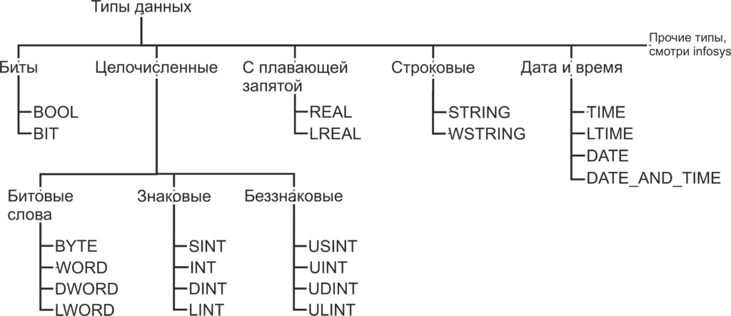
Биты
BOOL — это простейший тип данных, как уже было сказано, этот тип данных может принимать только два значения 0 и 1. Так же в TwinCAT, как и в большинстве языков программирования, эти значения, наравне с 0 и 1, обозначаются как TRUE и FALSE и несут в себе количество информации, соответствующее одному биту. Минимальным объемом данных, который читается из памяти за один раз, является байт, то есть восемь бит. Поэтому, для оптимизации скорости доступа к данным, переменная типа BOOL занимает восемь бит памяти. Для хранения самой переменной используется нулевой бит, а биты с первого по седьмой заполнены нулями. Впрочем, на практике о таком нюансе приходится вспоминать достаточно редко.
BIT — то же самое, что и BOOL, но в памяти занимает 1 бит. Как можно догадаться, операции с этим типом данных медленнее чем с типом BOOL, но он занимает меньше места в памяти. Тип данных BIT отсутствует в стандарте МЭК 61131-3 и поддерживается исключительно в TwinCAT, поэтому стоит отдавать предпочтение типу BOOL, когда у вас нет явных поводов использовать тип BIT.
Целочисленные типы данных
BYTE — тип данных, по размеру соответствующий одному байту. Хоть с типом BYTE можно производить математические операции, но в первую очередь он предназначен для хранения набора из 8 бит. Иногда в таком виде удобнее, чем побитно, передавать данные по цифровым интерфейсам, работать с входами выходами и так далее. С такими вопросами мы будем знакомится далее по мере изучения курса. В переменную типа BYTE можно записать числа из диапазона 0..255 (0..28-1).
WORD — то же самое, что и BYTE, но размером 16 бит. В переменную типа WORD можно записать числа из диапазона 0..65 535 (0..216-1). Тип данных WORD переводится с английского как «слово». Давным-давно термином машинное слово называли группу бит, обрабатываемых вычислительной машиной за один раз. Была уместна фраза «Программа состоит из машинных слов.». Со временем этим термином перестали пользоваться в прямом его значении, и сейчас под термином «машинное слово» обычно подразумевается группа из 16 бит.
DWORD — то же самое, что и BYTE, но размером 32 бит. В переменную типа DWORD можно записать числа из диапазона 0..4 294 967 295 (0..232-1). DWORD — это сокращение от double word, что переводится как двойное слово. Довольно часто буква «D» перед каким-либо типом данных значит, что этот тип данных в два раза длиннее, чем исходный.
LWORD — то же самое, что и BYTE, но размером 64 ;бит. В переменную типа LWORD можно записать числа из диапазона 0..18 446 744 073 709 551 615 (0..264-1). LWORD — это сокращение от long word, что переводится как длинное слово. Приставка «L» перед типом данных, как правило, означает что такой тип имеет длину 64 бита.
SINT — знаковый тип данных, длинной 8 бит. В переменную типа SINT можно записать числа из диапазона -128..127 (-27..27-1). В отличии от всех предыдущих типов данных этот тип данных предназначен для хранения именно чисел, а не набора бит. Слово знаковый в описании типа означает, что такой тип данных может хранить как положительные, так и отрицательные значения. Для хранения знака числа предназначен старший, в данном случае седьмой, разряд числа. Если старший разряд имеет значение 0, то число интерпретируется как положительное, если 1, то число интерпретируется как отрицательное. Приставка «S» означает short, что переводится с английского как короткий. Как вы догадались, SINT короткий вариант типа INT.
USINT — беззнаковый тип данных, длинной 8 бит. В переменную типа USINT можно записать числа из диапазона 0..255 (0..28-1). Приставка «U» означает unsigned, переводится как беззнаковый.
Остальные целочисленные типы аналогичны уже описанным и отличаются только размером. Сведем все целочисленные типы в таблицу.
| Тип данных | Нижний предел | Верхний предел | Занимаемая память |
| BYTE | 0 | 255 | 8 бит |
| WORD | 0 | 65 535 | 16 бит |
| DWORD | 0 | 4 294 967 295 | 32 бит |
| LWORD | 0 | 264-1 | 64 бит |
| SINT | -128 | 127 | 8 бит |
| USINT | 0 | 255 | 8 бит |
| INT | -32 768 | 32 767 | 16 бит |
| UINT | 0 | 65 535 | 16 бит |
| DINT | -2 147 483 648 | 2 147 483 647 | 32 бит |
| UDINT | 0 | 4 294 967 295 | 32 бит |
| LINT | -263 | -263-1 | 64 бит |
| ULINT | 0 | -264-1 | 64 бит |
Выше мы рассматривали целочисленные типы данных, то есть такие типы данных, в которых отсутствует запятая. При совершении математических операций с целочисленными типами данных есть некоторые особенности:
- Округление при делении: округление всегда выполняется вниз. То есть дробная часть просто отбрасывается. Если делимое меньше делителя, то частное всегда будет равно нулю, например, 10/11 = 0.
- Переполнение: если к целочисленной переменной, например, SINT, имеющей значение 255, прибавить 1, переменная переполнится и примет значение 0. Если прибавить 2, переменная примет значение 1 и так далее. При операции 0 — 1 результатом будет 255. Это свойство очень схоже с устройством стрелочных часов. Если сейчас 2 часа, то 5 часов назад было 9 часов. Только шкала часов имеет пределы не 1..12, а 0..255. Иногда такое свойство может использоваться при написании программ, но как правило не стоит допускать переполнения переменных.
Подробно такие нюансы разбираются в пособиях по дискретной математике. Мы на них пока что останавливаться не будем, но о приведенных двух особенностях не стоит забывать при написании программ.
Можно встретить упоминания о данных с фиксированной запятой, это такие данные, в которых количество знаков после запятой строго фиксировано. В TwinCAT типы данных с фиксированной запятой отсутствуют в чистом виде. TwinCAT поддерживает типы данных с плавающей запятой, то есть количество знаков до и после запятой может быть любым в пределах поддерживаемого диапазона.
Типы данных с плавающей запятой
REAL — тип данных с плавающей запятой длинной 32 бита. В переменную типа REAL можно записать числа из диапазона -3.402 82*1038..3.402 82*1038.
LREAL — тип данных с плавающей запятой длинной 64 бита. В переменную типа LREAL можно записать числа из диапазона -1.797 693 134 862 315 8*10308..1.797 693 134 862 315 8*10308.
При присваивании значения типам REAL и LREAL присваиваемое значение должно содержать целую часть, разделительную точку и дробную часть, например, 7.4 или 560.0.
Так же при записи значения типа REAL и LREAL использовать экспоненциальную (научную) форму. Примером экспоненциальной формы записи будет Me+P, в этом примере
- M называется мантиссой.
- e называется экспонентой (от англ. «exponent»), означающая «·10^» («…умножить на десять в степени…»),
- P называется порядком.
Примерами такой формы записи будет:
- 1.64e+3 расшифровывается как 1.64e+3 = 1.64*103 = 1640.
- 9.764e+5 расшифровывается как 9.764e+5 = 9.764*105 = 976400.
- 0.3694e+2 расшифровывается как 0.3694e+2 = 0.3694*102 = 36.94.
Еще один способ записи присваиваемого значения переменной типа REAL и LREAL, это добавить к числу префикс REAL#, например, REAL#7.4 или REAL#560. В таком случае можно не указывать дробную часть.
Старший, 31-й бит переменной типа REAL представляет собой знак. Следующие восемь бит, с 30-го по 23-й отведены под экспоненту. Оставшиеся 23 бита, с 22-го по 0-й используются для записи мантиссы.
В переменной типа LREAL старший, 63-й бит также используется для записи знака. В следующие 11 бит, с 62 по 52-й, записана экспонента. Оставшиеся 52 бита, с 51-го по 0-й, используются для записи мантиссы.
При записи числа с большим количеством значащих цифр в переменные типа REAL и LREAL производится округление. Необходимо не забывать об этом в расчетах, к которым предъявляются строгие требования по точности. Еще одна особенность, вытекающая из прошлой, если вы хотите сравнить два числа типа REAL или LREAL, прямое сравнение мало применимо, так как если в результате округления числа отличаются хоть на малую долю результат сравнения будет FALSE. Чтобы выполнить сравнение более корректно, можно вычесть одно число из другого, а потом оценить больше или меньше модуль получившегося результата вычитания, чем наибольшая допустимая разность. Поведение системы при переполнении переменных с плавающей запятой не определенно стандартом МЭК 61131-3, допускать его не стоит.
Строковые типы данных
STRING — тип данных для хранения символов. Каждый символ в переменной типа STRING хранится в 1 байте, в кодировке Windows-1252, это значит, что переменные такого типа поддерживают только латинские символы. При объявлении переменной количество символов в переменной указывается в круглых или квадратных скобках. Если размер не указан, при объявлении по умолчанию он равен 80 символам. Для данных типа STRING количество содержащихся в переменной символов не ограниченно, но функции для обработки строк могут принять до 255 символов.
Объем памяти, необходимый для переменной STRING, всегда составляет 1 байт на символ +1 дополнительный байт, например, переменная объявленная как «STRING [80]» будет занимать 81 байт. Для присвоения константного значения переменной типа STRING присваемый текст необходимо заключить в одинарные кавычки.
Пример объявления строки на 35 символов:
sVar : STRING(35) := 'This is a String'; (*Пример объявления переменной типа STRING*)
WSTRING — этот тип данных схож с типом STRING, но использует по 2 байта на символ и кодировку Unicode. Это значит что переменные типа WSTRING поддерживают символы кириллицы. Для присвоения константного значения переменной типа WSTRING присваемый текст необходимо заключить в двойные кавычки.
Пример объявления переменной типа WSTRING:
wsVar : WSTRING := "This is a WString"; (*Пример объявления переменной типа WSTRING*)Если значение, присваиваемое переменной STRING или WSTRING, содержит знак доллара ($), следующие два символа интерпретируются как шестнадцатеричный код в соответствии с кодировкой Windows-1252. Код также соответствует кодировке ASCII.
| Код со знаком доллара | Его значение в переменной |
| $<восьмибитное число> | Восьмибитное число интерпретируется как символ в кодировке ISO / IEC 8859-1 |
| ‘$41’ | A |
| ‘$9A’ | © |
| ‘$40’ | @ |
| ‘$0D’, ‘$R’, ‘$r’ | Разрыв строки |
| ‘$0A’, ‘$L’, ‘$l’, ‘$N’, ‘$n’ | Новая строка |
| ‘$P’, ‘$p’ | Конец страницы |
| ‘$T’, ‘$t’ | Табуляция |
| ‘$$’ | Знак доллара |
| ‘$’ ‘ | Одиночная кавычка |
Такое разнообразие кодировок связанно с тем, что у всех из них первые 128 символов соответствуют кодовой таблице ASCII, но в статье для каждого случая кодировка указывалась так же, как она указана в infosys.
Пример:
VAR CONSTANT
sConstA : STRING :='Hello world';
sConstB : STRING :='Hello world $21'; (*Пример объявления переменной типа STRING с спец символом*)
END_VAR
Типы данных времени
TIME — тип данных, предназначенный для хранения временных промежутков. Размер типа данных 32 бита. Этот тип данных интерпретируется в TwinCAT, как переменная типа DWORD, содержащая время в миллисекундах. Нижний допустимый предел 0 (0 мс), верхний предел 4 294 967 295 (49 дней, 17 часов, 2 минуты, 47 секунд, 295 миллисекунд). Для записи значений в переменные типа TIME используется префикс T# и суффиксы d: дни, h: часы, m: минуты, s: секунды, ms: миллисекунды, которые должны располагаться в порядке убывания.
Примеры корректного присваивания значения переменной типа TIME:
TIME1 : TIME := T#14ms;
TIME1 : TIME := T#100s12ms; // Допускается переполнение в старшем отрезке времени.
TIME1 : TIME := t#12h34m15s;
Примеры некорректного присваивания значения переменной типа TIME, при компиляции будет выдана ошибка:
TIME1 : TIME := t#5m68s;   // Переполнение не в старшем отрезке времени недопустимо
TIME1 : TIME := 15ms;   // Пропущен префикс T#
TIME1 : TIME := t#4ms13d;   // Не соблюден порядок записи временных отрезок
LTIME — тип данных аналогичен TIME, но его размер составляет 64 бита, а временные отрезки хранятся в наносекундах. Нижний допустимый предел 0, верхний предел 213 503 дней, 23 часов, 34 минуты, 33 секунд, 709 миллисекунд, 551 микросекунд и 615 наносекунд. Для записи значений в переменные типа LTIME используется префикс LTIME#. Помимо суффиксов, используемых для записи типа TIME для LTIME, используются µs: микросекунды и ns: наносекунды.
Пример:
LTIME1 : LTIME := LTIME#1000d15h23m12s34ms2us44ns; (*Пример объявления переменной типа LTIME*)TIME_OF_DAY (TOD) — тип данных для записи времени суток. Имеет размер 32 бита. Нижнее допустимое значение 0, верхнее допустимое значение 23 часа, 59 минут, 59 секунд, 999 миллисекунд. Для записи значений в переменные типа TOD используется префикс TIME_OF_DAY# или TOD#, значение записывается в виде <часы : минуты : секунды> . В остальном этот тип данных аналогичен типу TIME.
Пример:
TIME_OF_DAY#15:36:30.123
tod#00:00:00
Date — тип данных для записи даты. Имеет размер 32 бита. Нижнее допустимое значение 0 (01.01.1970), верхнее допустимое значение 4 294 967 295 (7 февраля 2106), да, здесь присутствует возможный компьютерный апокалипсис, но учитывая запас по верхнему пределу, эта проблема не слишком актуальна. Для записи значений в переменные типа TOD используется префикс DATE# или D#, значение записывается в виде <год — месяц — дата>. В остальном этот тип данных аналогичен типу TIME.
DATE#1996-05-06
d#1972-03-29
DATE_AND_TIME (DT) — тип данных для записи даты и времени. Имеет размер 32 бита. Нижнее допустимое значение 0 (01.01.1970), верхнее допустимое значение 4 294 967 295 (7 февраля 2106, 6:28:15). Для записи значений в переменные типа DT используется префикс DATE_AND_TIME # или DT#, значение записывается в виде <год — месяц — дата — час : минута : секунда>. В остальном этот тип данных аналогичен типу TIME.
DATE_AND_TIME#1996-05-06-15:36:30
dt#1972-03-29-00:00:00
На этом раз мы заканчиваем рассмотрение типов данных. Сейчас мы разобрали не все типы данных, остальные можно найти в infosys по пути TwinCAT 3 → TE1000 XAE → PLC → Reference Programming → Data types.
Следующая статья будет целиком состоять из практической работы, мы напишем калькулятор на языке LD.
From Wikipedia, the free encyclopedia
In computing, a word is the natural unit of data used by a particular processor design. A word is a fixed-sized datum handled as a unit by the instruction set or the hardware of the processor. The number of bits or digits[a] in a word (the word size, word width, or word length) is an important characteristic of any specific processor design or computer architecture.
The size of a word is reflected in many aspects of a computer’s structure and operation; the majority of the registers in a processor are usually word-sized and the largest datum that can be transferred to and from the working memory in a single operation is a word in many (not all) architectures. The largest possible address size, used to designate a location in memory, is typically a hardware word (here, «hardware word» means the full-sized natural word of the processor, as opposed to any other definition used).
Documentation for older computers with fixed word size commonly states memory sizes in words rather than bytes or characters. The documentation sometimes uses metric prefixes correctly, sometimes with rounding, e.g., 65 kilowords (KW) meaning for 65536 words, and sometimes uses them incorrectly, with kilowords (KW) meaning 1024 words (210) and megawords (MW) meaning 1,048,576 words (220). With standardization on 8-bit bytes and byte addressability, stating memory sizes in bytes, kilobytes, and megabytes with powers of 1024 rather than 1000 has become the norm, although there is some use of the IEC binary prefixes.
Several of the earliest computers (and a few modern as well) use binary-coded decimal rather than plain binary, typically having a word size of 10 or 12 decimal digits, and some early decimal computers have no fixed word length at all. Early binary systems tended to use word lengths that were some multiple of 6-bits, with the 36-bit word being especially common on mainframe computers. The introduction of ASCII led to the move to systems with word lengths that were a multiple of 8-bits, with 16-bit machines being popular in the 1970s before the move to modern processors with 32 or 64 bits.[1] Special-purpose designs like digital signal processors, may have any word length from 4 to 80 bits.[1]
The size of a word can sometimes differ from the expected due to backward compatibility with earlier computers. If multiple compatible variations or a family of processors share a common architecture and instruction set but differ in their word sizes, their documentation and software may become notationally complex to accommodate the difference (see Size families below).
Uses of words[edit]
Depending on how a computer is organized, word-size units may be used for:
- Fixed-point numbers
- Holders for fixed point, usually integer, numerical values may be available in one or in several different sizes, but one of the sizes available will almost always be the word. The other sizes, if any, are likely to be multiples or fractions of the word size. The smaller sizes are normally used only for efficient use of memory; when loaded into the processor, their values usually go into a larger, word sized holder.
- Floating-point numbers
- Holders for floating-point numerical values are typically either a word or a multiple of a word.
- Addresses
- Holders for memory addresses must be of a size capable of expressing the needed range of values but not be excessively large, so often the size used is the word though it can also be a multiple or fraction of the word size.
- Registers
- Processor registers are designed with a size appropriate for the type of data they hold, e.g. integers, floating-point numbers, or addresses. Many computer architectures use general-purpose registers that are capable of storing data in multiple representations.
- Memory–processor transfer
- When the processor reads from the memory subsystem into a register or writes a register’s value to memory, the amount of data transferred is often a word. Historically, this amount of bits which could be transferred in one cycle was also called a catena in some environments (such as the Bull GAMMA 60 [fr]).[2][3] In simple memory subsystems, the word is transferred over the memory data bus, which typically has a width of a word or half-word. In memory subsystems that use caches, the word-sized transfer is the one between the processor and the first level of cache; at lower levels of the memory hierarchy larger transfers (which are a multiple of the word size) are normally used.
- Unit of address resolution
- In a given architecture, successive address values designate successive units of memory; this unit is the unit of address resolution. In most computers, the unit is either a character (e.g. a byte) or a word. (A few computers have used bit resolution.) If the unit is a word, then a larger amount of memory can be accessed using an address of a given size at the cost of added complexity to access individual characters. On the other hand, if the unit is a byte, then individual characters can be addressed (i.e. selected during the memory operation).
- Instructions
- Machine instructions are normally the size of the architecture’s word, such as in RISC architectures, or a multiple of the «char» size that is a fraction of it. This is a natural choice since instructions and data usually share the same memory subsystem. In Harvard architectures the word sizes of instructions and data need not be related, as instructions and data are stored in different memories; for example, the processor in the 1ESS electronic telephone switch has 37-bit instructions and 23-bit data words.
Word size choice[edit]
When a computer architecture is designed, the choice of a word size is of substantial importance. There are design considerations which encourage particular bit-group sizes for particular uses (e.g. for addresses), and these considerations point to different sizes for different uses. However, considerations of economy in design strongly push for one size, or a very few sizes related by multiples or fractions (submultiples) to a primary size. That preferred size becomes the word size of the architecture.
Character size was in the past (pre-variable-sized character encoding) one of the influences on unit of address resolution and the choice of word size. Before the mid-1960s, characters were most often stored in six bits; this allowed no more than 64 characters, so the alphabet was limited to upper case. Since it is efficient in time and space to have the word size be a multiple of the character size, word sizes in this period were usually multiples of 6 bits (in binary machines). A common choice then was the 36-bit word, which is also a good size for the numeric properties of a floating point format.
After the introduction of the IBM System/360 design, which uses eight-bit characters and supports lower-case letters, the standard size of a character (or more accurately, a byte) becomes eight bits. Word sizes thereafter are naturally multiples of eight bits, with 16, 32, and 64 bits being commonly used.
Variable-word architectures[edit]
Early machine designs included some that used what is often termed a variable word length. In this type of organization, an operand has no fixed length. Depending on the machine and the instruction, the length might be denoted by a count field, by a delimiting character, or by an additional bit called, e.g., flag, or word mark. Such machines often use binary-coded decimal in 4-bit digits, or in 6-bit characters, for numbers. This class of machines includes the IBM 702, IBM 705, IBM 7080, IBM 7010, UNIVAC 1050, IBM 1401, IBM 1620, and RCA 301.
Most of these machines work on one unit of memory at a time and since each instruction or datum is several units long, each instruction takes several cycles just to access memory. These machines are often quite slow because of this. For example, instruction fetches on an IBM 1620 Model I take 8 cycles (160 μs) just to read the 12 digits of the instruction (the Model II reduced this to 6 cycles, or 4 cycles if the instruction did not need both address fields). Instruction execution takes a variable number of cycles, depending on the size of the operands.
Word, bit and byte addressing[edit]
The memory model of an architecture is strongly influenced by the word size. In particular, the resolution of a memory address, that is, the smallest unit that can be designated by an address, has often been chosen to be the word. In this approach, the word-addressable machine approach, address values which differ by one designate adjacent memory words. This is natural in machines which deal almost always in word (or multiple-word) units, and has the advantage of allowing instructions to use minimally sized fields to contain addresses, which can permit a smaller instruction size or a larger variety of instructions.
When byte processing is to be a significant part of the workload, it is usually more advantageous to use the byte, rather than the word, as the unit of address resolution. Address values which differ by one designate adjacent bytes in memory. This allows an arbitrary character within a character string to be addressed straightforwardly. A word can still be addressed, but the address to be used requires a few more bits than the word-resolution alternative. The word size needs to be an integer multiple of the character size in this organization. This addressing approach was used in the IBM 360, and has been the most common approach in machines designed since then.
When the workload involves processing fields of different sizes, it can be advantageous to address to the bit. Machines with bit addressing may have some instructions that use a programmer-defined byte size and other instructions that operate on fixed data sizes. As an example, on the IBM 7030[4] («Stretch»), a floating point instruction can only address words while an integer arithmetic instruction can specify a field length of 1-64 bits, a byte size of 1-8 bits and an accumulator offset of 0-127 bits.
In a byte-addressable machine with storage-to-storage (SS) instructions, there are typically move instructions to copy one or multiple bytes from one arbitrary location to another. In a byte-oriented (byte-addressable) machine without SS instructions, moving a single byte from one arbitrary location to another is typically:
- LOAD the source byte
- STORE the result back in the target byte
Individual bytes can be accessed on a word-oriented machine in one of two ways. Bytes can be manipulated by a combination of shift and mask operations in registers. Moving a single byte from one arbitrary location to another may require the equivalent of the following:
- LOAD the word containing the source byte
- SHIFT the source word to align the desired byte to the correct position in the target word
- AND the source word with a mask to zero out all but the desired bits
- LOAD the word containing the target byte
- AND the target word with a mask to zero out the target byte
- OR the registers containing the source and target words to insert the source byte
- STORE the result back in the target location
Alternatively many word-oriented machines implement byte operations with instructions using special byte pointers in registers or memory. For example, the PDP-10 byte pointer contained the size of the byte in bits (allowing different-sized bytes to be accessed), the bit position of the byte within the word, and the word address of the data. Instructions could automatically adjust the pointer to the next byte on, for example, load and deposit (store) operations.
Powers of two[edit]
Different amounts of memory are used to store data values with different degrees of precision. The commonly used sizes are usually a power of two multiple of the unit of address resolution (byte or word). Converting the index of an item in an array into the memory address offset of the item then requires only a shift operation rather than a multiplication. In some cases this relationship can also avoid the use of division operations. As a result, most modern computer designs have word sizes (and other operand sizes) that are a power of two times the size of a byte.
Size families[edit]
As computer designs have grown more complex, the central importance of a single word size to an architecture has decreased. Although more capable hardware can use a wider variety of sizes of data, market forces exert pressure to maintain backward compatibility while extending processor capability. As a result, what might have been the central word size in a fresh design has to coexist as an alternative size to the original word size in a backward compatible design. The original word size remains available in future designs, forming the basis of a size family.
In the mid-1970s, DEC designed the VAX to be a 32-bit successor of the 16-bit PDP-11. They used word for a 16-bit quantity, while longword referred to a 32-bit quantity; this terminology is the same as the terminology used for the PDP-11. This was in contrast to earlier machines, where the natural unit of addressing memory would be called a word, while a quantity that is one half a word would be called a halfword. In fitting with this scheme, a VAX quadword is 64 bits. They continued this 16-bit word/32-bit longword/64-bit quadword terminology with the 64-bit Alpha.
Another example is the x86 family, of which processors of three different word lengths (16-bit, later 32- and 64-bit) have been released, while word continues to designate a 16-bit quantity. As software is routinely ported from one word-length to the next, some APIs and documentation define or refer to an older (and thus shorter) word-length than the full word length on the CPU that software may be compiled for. Also, similar to how bytes are used for small numbers in many programs, a shorter word (16 or 32 bits) may be used in contexts where the range of a wider word is not needed (especially where this can save considerable stack space or cache memory space). For example, Microsoft’s Windows API maintains the programming language definition of WORD as 16 bits, despite the fact that the API may be used on a 32- or 64-bit x86 processor, where the standard word size would be 32 or 64 bits, respectively. Data structures containing such different sized words refer to them as:
- WORD (16 bits/2 bytes)
- DWORD (32 bits/4 bytes)
- QWORD (64 bits/8 bytes)
A similar phenomenon has developed in Intel’s x86 assembly language – because of the support for various sizes (and backward compatibility) in the instruction set, some instruction mnemonics carry «d» or «q» identifiers denoting «double-«, «quad-» or «double-quad-«, which are in terms of the architecture’s original 16-bit word size.
An example with a different word size is the IBM System/360 family. In the System/360 architecture, System/370 architecture and System/390 architecture, there are 8-bit bytes, 16-bit halfwords, 32-bit words and 64-bit doublewords. The z/Architecture, which is the 64-bit member of that architecture family, continues to refer to 16-bit halfwords, 32-bit words, and 64-bit doublewords, and additionally features 128-bit quadwords.
In general, new processors must use the same data word lengths and virtual address widths as an older processor to have binary compatibility with that older processor.
Often carefully written source code – written with source-code compatibility and software portability in mind – can be recompiled to run on a variety of processors, even ones with different data word lengths or different address widths or both.
Table of word sizes[edit]
| key: bit: bits, c: characters, d: decimal digits, w: word size of architecture, n: variable size, wm: Word mark | |||||||
|---|---|---|---|---|---|---|---|
| Year | Computer architecture |
Word size w | Integer sizes |
Floatingpoint sizes |
Instruction sizes |
Unit of address resolution |
Char size |
| 1837 | Babbage Analytical engine |
50 d | w | — | Five different cards were used for different functions, exact size of cards not known. | w | — |
| 1941 | Zuse Z3 | 22 bit | — | w | 8 bit | w | — |
| 1942 | ABC | 50 bit | w | — | — | — | — |
| 1944 | Harvard Mark I | 23 d | w | — | 24 bit | — | — |
| 1946 (1948) {1953} |
ENIAC (w/Panel #16[5]) {w/Panel #26[6]} |
10 d | w, 2w (w) {w} |
— | — (2 d, 4 d, 6 d, 8 d) {2 d, 4 d, 6 d, 8 d} |
— — {w} |
— |
| 1948 | Manchester Baby | 32 bit | w | — | w | w | — |
| 1951 | UNIVAC I | 12 d | w | — | 1⁄2w | w | 1 d |
| 1952 | IAS machine | 40 bit | w | — | 1⁄2w | w | 5 bit |
| 1952 | Fast Universal Digital Computer M-2 | 34 bit | w? | w | 34 bit = 4-bit opcode plus 3×10 bit address | 10 bit | — |
| 1952 | IBM 701 | 36 bit | 1⁄2w, w | — | 1⁄2w | 1⁄2w, w | 6 bit |
| 1952 | UNIVAC 60 | n d | 1 d, … 10 d | — | — | — | 2 d, 3 d |
| 1952 | ARRA I | 30 bit | w | — | w | w | 5 bit |
| 1953 | IBM 702 | n c | 0 c, … 511 c | — | 5 c | c | 6 bit |
| 1953 | UNIVAC 120 | n d | 1 d, … 10 d | — | — | — | 2 d, 3 d |
| 1953 | ARRA II | 30 bit | w | 2w | 1⁄2w | w | 5 bit |
| 1954 (1955) |
IBM 650 (w/IBM 653) |
10 d | w | — (w) |
w | w | 2 d |
| 1954 | IBM 704 | 36 bit | w | w | w | w | 6 bit |
| 1954 | IBM 705 | n c | 0 c, … 255 c | — | 5 c | c | 6 bit |
| 1954 | IBM NORC | 16 d | w | w, 2w | w | w | — |
| 1956 | IBM 305 | n d | 1 d, … 100 d | — | 10 d | d | 1 d |
| 1956 | ARMAC | 34 bit | w | w | 1⁄2w | w | 5 bit, 6 bit |
| 1956 | LGP-30 | 31 bit | w | — | 16 bit | w | 6 bit |
| 1957 | Autonetics Recomp I | 40 bit | w, 79 bit, 8 d, 15 d | — | 1⁄2w | 1⁄2w, w | 5 bit |
| 1958 | UNIVAC II | 12 d | w | — | 1⁄2w | w | 1 d |
| 1958 | SAGE | 32 bit | 1⁄2w | — | w | w | 6 bit |
| 1958 | Autonetics Recomp II | 40 bit | w, 79 bit, 8 d, 15 d | 2w | 1⁄2w | 1⁄2w, w | 5 bit |
| 1958 | Setun | 6 trit (~9.5 bits)[b] | up to 6 tryte | up to 3 trytes | 4 trit? | ||
| 1958 | Electrologica X1 | 27 bit | w | 2w | w | w | 5 bit, 6 bit |
| 1959 | IBM 1401 | n c | 1 c, … | — | 1 c, 2 c, 4 c, 5 c, 7 c, 8 c | c | 6 bit + wm |
| 1959 (TBD) |
IBM 1620 | n d | 2 d, … | — (4 d, … 102 d) |
12 d | d | 2 d |
| 1960 | LARC | 12 d | w, 2w | w, 2w | w | w | 2 d |
| 1960 | CDC 1604 | 48 bit | w | w | 1⁄2w | w | 6 bit |
| 1960 | IBM 1410 | n c | 1 c, … | — | 1 c, 2 c, 6 c, 7 c, 11 c, 12 c | c | 6 bit + wm |
| 1960 | IBM 7070 | 10 d[c] | w, 1-9 d | w | w | w, d | 2 d |
| 1960 | PDP-1 | 18 bit | w | — | w | w | 6 bit |
| 1960 | Elliott 803 | 39 bit | |||||
| 1961 | IBM 7030 (Stretch) |
64 bit | 1 bit, … 64 bit, 1 d, … 16 d |
w | 1⁄2w, w | bit (integer), 1⁄2w (branch), w (float) |
1 bit, … 8 bit |
| 1961 | IBM 7080 | n c | 0 c, … 255 c | — | 5 c | c | 6 bit |
| 1962 | GE-6xx | 36 bit | w, 2 w | w, 2 w, 80 bit | w | w | 6 bit, 9 bit |
| 1962 | UNIVAC III | 25 bit | w, 2w, 3w, 4w, 6 d, 12 d | — | w | w | 6 bit |
| 1962 | Autonetics D-17B Minuteman I Guidance Computer |
27 bit | 11 bit, 24 bit | — | 24 bit | w | — |
| 1962 | UNIVAC 1107 | 36 bit | 1⁄6w, 1⁄3w, 1⁄2w, w | w | w | w | 6 bit |
| 1962 | IBM 7010 | n c | 1 c, … | — | 1 c, 2 c, 6 c, 7 c, 11 c, 12 c | c | 6 b + wm |
| 1962 | IBM 7094 | 36 bit | w | w, 2w | w | w | 6 bit |
| 1962 | SDS 9 Series | 24 bit | w | 2w | w | w | |
| 1963 (1966) |
Apollo Guidance Computer | 15 bit | w | — | w, 2w | w | — |
| 1963 | Saturn Launch Vehicle Digital Computer | 26 bit | w | — | 13 bit | w | — |
| 1964/1966 | PDP-6/PDP-10 | 36 bit | w | w, 2 w | w | w | 6 bit 7 bit (typical) 9 bit |
| 1964 | Titan | 48 bit | w | w | w | w | w |
| 1964 | CDC 6600 | 60 bit | w | w | 1⁄4w, 1⁄2w | w | 6 bit |
| 1964 | Autonetics D-37C Minuteman II Guidance Computer |
27 bit | 11 bit, 24 bit | — | 24 bit | w | 4 bit, 5 bit |
| 1965 | Gemini Guidance Computer | 39 bit | 26 bit | — | 13 bit | 13 bit, 26 | —bit |
| 1965 | IBM 1130 | 16 bit | w, 2w | 2w, 3w | w, 2w | w | 8 bit |
| 1965 | IBM System/360 | 32 bit | 1⁄2w, w, 1 d, … 16 d |
w, 2w | 1⁄2w, w, 11⁄2w | 8 bit | 8 bit |
| 1965 | UNIVAC 1108 | 36 bit | 1⁄6w, 1⁄4w, 1⁄3w, 1⁄2w, w, 2w | w, 2w | w | w | 6 bit, 9 bit |
| 1965 | PDP-8 | 12 bit | w | — | w | w | 8 bit |
| 1965 | Electrologica X8 | 27 bit | w | 2w | w | w | 6 bit, 7 bit |
| 1966 | SDS Sigma 7 | 32 bit | 1⁄2w, w | w, 2w | w | 8 bit | 8 bit |
| 1969 | Four-Phase Systems AL1 | 8 bit | w | — | ? | ? | ? |
| 1970 | MP944 | 20 bit | w | — | ? | ? | ? |
| 1970 | PDP-11 | 16 bit | w | 2w, 4w | w, 2w, 3w | 8 bit | 8 bit |
| 1971 | CDC STAR-100 | 64 bit | 1⁄2w, w | 1⁄2w, w | 1⁄2w, w | bit | 8 bit |
| 1971 | TMS1802NC | 4 bit | w | — | ? | ? | — |
| 1971 | Intel 4004 | 4 bit | w, d | — | 2w, 4w | w | — |
| 1972 | Intel 8008 | 8 bit | w, 2 d | — | w, 2w, 3w | w | 8 bit |
| 1972 | Calcomp 900 | 9 bit | w | — | w, 2w | w | 8 bit |
| 1974 | Intel 8080 | 8 bit | w, 2w, 2 d | — | w, 2w, 3w | w | 8 bit |
| 1975 | ILLIAC IV | 64 bit | w | w, 1⁄2w | w | w | — |
| 1975 | Motorola 6800 | 8 bit | w, 2 d | — | w, 2w, 3w | w | 8 bit |
| 1975 | MOS Tech. 6501 MOS Tech. 6502 |
8 bit | w, 2 d | — | w, 2w, 3w | w | 8 bit |
| 1976 | Cray-1 | 64 bit | 24 bit, w | w | 1⁄4w, 1⁄2w | w | 8 bit |
| 1976 | Zilog Z80 | 8 bit | w, 2w, 2 d | — | w, 2w, 3w, 4w, 5w | w | 8 bit |
| 1978 (1980) |
16-bit x86 (Intel 8086) (w/floating point: Intel 8087) |
16 bit | 1⁄2w, w, 2 d | — (2w, 4w, 5w, 17 d) |
1⁄2w, w, … 7w | 8 bit | 8 bit |
| 1978 | VAX | 32 bit | 1⁄4w, 1⁄2w, w, 1 d, … 31 d, 1 bit, … 32 bit | w, 2w | 1⁄4w, … 141⁄4w | 8 bit | 8 bit |
| 1979 (1984) |
Motorola 68000 series (w/floating point) |
32 bit | 1⁄4w, 1⁄2w, w, 2 d | — (w, 2w, 21⁄2w) |
1⁄2w, w, … 71⁄2w | 8 bit | 8 bit |
| 1985 | IA-32 (Intel 80386) (w/floating point) | 32 bit | 1⁄4w, 1⁄2w, w | — (w, 2w, 80 bit) |
8 bit, … 120 bit 1⁄4w … 33⁄4w |
8 bit | 8 bit |
| 1985 | ARMv1 | 32 bit | 1⁄4w, w | — | w | 8 bit | 8 bit |
| 1985 | MIPS I | 32 bit | 1⁄4w, 1⁄2w, w | w, 2w | w | 8 bit | 8 bit |
| 1991 | Cray C90 | 64 bit | 32 bit, w | w | 1⁄4w, 1⁄2w, 48 bit | w | 8 bit |
| 1992 | Alpha | 64 bit | 8 bit, 1⁄4w, 1⁄2w, w | 1⁄2w, w | 1⁄2w | 8 bit | 8 bit |
| 1992 | PowerPC | 32 bit | 1⁄4w, 1⁄2w, w | w, 2w | w | 8 bit | 8 bit |
| 1996 | ARMv4 (w/Thumb) |
32 bit | 1⁄4w, 1⁄2w, w | — | w (1⁄2w, w) |
8 bit | 8 bit |
| 2000 | IBM z/Architecture (w/vector facility) |
64 bit | 1⁄4w, 1⁄2w, w 1 d, … 31 d |
1⁄2w, w, 2w | 1⁄4w, 1⁄2w, 3⁄4w | 8 bit | 8 bit, UTF-16, UTF-32 |
| 2001 | IA-64 | 64 bit | 8 bit, 1⁄4w, 1⁄2w, w | 1⁄2w, w | 41 bit (in 128-bit bundles)[7] | 8 bit | 8 bit |
| 2001 | ARMv6 (w/VFP) |
32 bit | 8 bit, 1⁄2w, w | — (w, 2w) |
1⁄2w, w | 8 bit | 8 bit |
| 2003 | x86-64 | 64 bit | 8 bit, 1⁄4w, 1⁄2w, w | 1⁄2w, w, 80 bit | 8 bit, … 120 bit | 8 bit | 8 bit |
| 2013 | ARMv8-A and ARMv9-A | 64 bit | 8 bit, 1⁄4w, 1⁄2w, w | 1⁄2w, w | 1⁄2w | 8 bit | 8 bit |
| Year | Computer architecture |
Word size w | Integer sizes |
Floatingpoint sizes |
Instruction sizes |
Unit of address resolution |
Char size |
| key: bit: bits, d: decimal digits, w: word size of architecture, n: variable size |
[8][9]
See also[edit]
- Integer (computer science)
Notes[edit]
- ^ Many early computers were decimal, and a few were ternary
- ^ The bit equivalent is computed by taking the amount of information entropy provided by the trit, which is
 . This gives an equivalent of about 9.51 bits for 6 trits.
- ^ Three-state sign

References[edit]
- ^ a b Beebe, Nelson H. F. (2017-08-22). «Chapter I. Integer arithmetic». The Mathematical-Function Computation Handbook — Programming Using the MathCW Portable Software Library (1 ed.). Salt Lake City, UT, USA: Springer International Publishing AG. p. 970. doi:10.1007/978-3-319-64110-2. ISBN 978-3-319-64109-6. LCCN 2017947446. S2CID 30244721.
- ^ Dreyfus, Phillippe (1958-05-08) [1958-05-06]. Written at Los Angeles, California, USA. System design of the Gamma 60 (PDF). Western Joint Computer Conference: Contrasts in Computers. ACM, New York, NY, USA. pp. 130–133. IRE-ACM-AIEE ’58 (Western). Archived (PDF) from the original on 2017-04-03. Retrieved 2017-04-03.
[…] Internal data code is used: Quantitative (numerical) data are coded in a 4-bit decimal code; qualitative (alpha-numerical) data are coded in a 6-bit alphanumerical code. The internal instruction code means that the instructions are coded in straight binary code.
As to the internal information length, the information quantum is called a «catena,» and it is composed of 24 bits representing either 6 decimal digits, or 4 alphanumerical characters. This quantum must contain a multiple of 4 and 6 bits to represent a whole number of decimal or alphanumeric characters. Twenty-four bits was found to be a good compromise between the minimum 12 bits, which would lead to a too-low transfer flow from a parallel readout core memory, and 36 bits or more, which was judged as too large an information quantum. The catena is to be considered as the equivalent of a character in variable word length machines, but it cannot be called so, as it may contain several characters. It is transferred in series to and from the main memory.
Not wanting to call a «quantum» a word, or a set of characters a letter, (a word is a word, and a quantum is something else), a new word was made, and it was called a «catena.» It is an English word and exists in Webster’s although it does not in French. Webster’s definition of the word catena is, «a connected series;» therefore, a 24-bit information item. The word catena will be used hereafter.
The internal code, therefore, has been defined. Now what are the external data codes? These depend primarily upon the information handling device involved. The Gamma 60 [fr] is designed to handle information relevant to any binary coded structure. Thus an 80-column punched card is considered as a 960-bit information item; 12 rows multiplied by 80 columns equals 960 possible punches; is stored as an exact image in 960 magnetic cores of the main memory with 2 card columns occupying one catena. […] - ^ Blaauw, Gerrit Anne; Brooks, Jr., Frederick Phillips; Buchholz, Werner (1962). «4: Natural Data Units» (PDF). In Buchholz, Werner (ed.). Planning a Computer System – Project Stretch. McGraw-Hill Book Company, Inc. / The Maple Press Company, York, PA. pp. 39–40. LCCN 61-10466. Archived (PDF) from the original on 2017-04-03. Retrieved 2017-04-03.
[…] Terms used here to describe the structure imposed by the machine design, in addition to bit, are listed below.
Byte denotes a group of bits used to encode a character, or the number of bits transmitted in parallel to and from input-output units. A term other than character is used here because a given character may be represented in different applications by more than one code, and different codes may use different numbers of bits (i.e., different byte sizes). In input-output transmission the grouping of bits may be completely arbitrary and have no relation to actual characters. (The term is coined from bite, but respelled to avoid accidental mutation to bit.)
A word consists of the number of data bits transmitted in parallel from or to memory in one memory cycle. Word size is thus defined as a structural property of the memory. (The term catena was coined for this purpose by the designers of the Bull GAMMA 60 [fr] computer.)
Block refers to the number of words transmitted to or from an input-output unit in response to a single input-output instruction. Block size is a structural property of an input-output unit; it may have been fixed by the design or left to be varied by the program. […] - ^ «Format» (PDF). Reference Manual 7030 Data Processing System (PDF). IBM. August 1961. pp. 50–57. Retrieved 2021-12-15.
- ^ Clippinger, Richard F. [in German] (1948-09-29). «A Logical Coding System Applied to the ENIAC (Electronic Numerical Integrator and Computer)». Aberdeen Proving Ground, Maryland, US: Ballistic Research Laboratories. Report No. 673; Project No. TB3-0007 of the Research and Development Division, Ordnance Department. Retrieved 2017-04-05.
{{cite web}}: CS1 maint: url-status (link) - ^ Clippinger, Richard F. [in German] (1948-09-29). «A Logical Coding System Applied to the ENIAC». Aberdeen Proving Ground, Maryland, US: Ballistic Research Laboratories. Section VIII: Modified ENIAC. Retrieved 2017-04-05.
{{cite web}}: CS1 maint: url-status (link) - ^ «4. Instruction Formats» (PDF). Intel Itanium Architecture Software Developer’s Manual. Vol. 3: Intel Itanium Instruction Set Reference. p. 3:293. Retrieved 2022-04-25.
Three instructions are grouped together into 128-bit sized and aligned containers called bundles. Each bundle contains three 41-bit instruction slots and a 5-bit template field.
- ^ Blaauw, Gerrit Anne; Brooks, Jr., Frederick Phillips (1997). Computer Architecture: Concepts and Evolution (1 ed.). Addison-Wesley. ISBN 0-201-10557-8. (1213 pages) (NB. This is a single-volume edition. This work was also available in a two-volume version.)
- ^ Ralston, Anthony; Reilly, Edwin D. (1993). Encyclopedia of Computer Science (3rd ed.). Van Nostrand Reinhold. ISBN 0-442-27679-6.
│
Deutsch (de) │
English (en) │
suomi (fi) │
français (fr) │
русский (ru) │
A word is the processor’s native data unit.
Modern consumer processors have a word width of 64 bits.
Data type
Most run-time libraries provide the native data type of a processor as the Pascal data type word.
It is a subset of all whole numbers (non-negative integers) that can be represented by the processor’s natural data unit size.
On a 64-bit architecture this means a word is an integer within the range [math]displaystyle{ [0,~2^{64}-1] }[/math].
On a 32-bit architecture a word will be an integer in the range [math]displaystyle{ [0,~2^{32}-1] }[/math], and so on, respectively.
In GNU Pascal a word is just an alias for cardinal, which has the same properties regarding possible values.
If a signed integer having the processor’s native size is wanted, the data type integer provides this functionality.
FPC
For source compatibility reasons, FPC defines word in the same way as Turbo Pascal and Delphi: the subrange data type 0..65535.
The high value 65535 is [math]displaystyle{ 2^{16}-1 }[/math].
Thus a system.word occupies two bytes of space.
Subrange data types are stored in a quantity that serves best the goals of performance and memory efficiency.
The processor’s native word size, as defined above, corresponds to different types depending on the purpose you want to use it for:
- the (as of 2022 still undocumented)
system.ALUSintandsystem.ALUUinttypes correspond to the native word size used by the processor’s ALU (arithmetic and logical unit), as defined at the beginning of this page. In general, this type should not be used in high level code. Instead, choose a data type based on the values it should be able to represent, as this is safer and more portable. It is the compiler’s job to generate optimal code. system.CodePtrUIntcorresponds to the size of pointers to code, such as the address of a procedure. This can be different from a pointer to data, e. g. on targets that support multiple memory models.system.PtrUIntcorresponds to the size of pointers to data.
On many platforms, all of these types have the same size, but it is not the case everywhere.
In FPC a smallInt has the same size as a word, but is signed.
| simple data types |
|
|---|---|
| complex data types |
|
From Wikipedia, the free encyclopedia
In computing, a word is the natural unit of data used by a particular processor design. A word is a fixed-sized datum handled as a unit by the instruction set or the hardware of the processor. The number of bits or digits[a] in a word (the word size, word width, or word length) is an important characteristic of any specific processor design or computer architecture.
The size of a word is reflected in many aspects of a computer’s structure and operation; the majority of the registers in a processor are usually word-sized and the largest datum that can be transferred to and from the working memory in a single operation is a word in many (not all) architectures. The largest possible address size, used to designate a location in memory, is typically a hardware word (here, «hardware word» means the full-sized natural word of the processor, as opposed to any other definition used).
Documentation for older computers with fixed word size commonly states memory sizes in words rather than bytes or characters. The documentation sometimes uses metric prefixes correctly, sometimes with rounding, e.g., 65 kilowords (KW) meaning for 65536 words, and sometimes uses them incorrectly, with kilowords (KW) meaning 1024 words (210) and megawords (MW) meaning 1,048,576 words (220). With standardization on 8-bit bytes and byte addressability, stating memory sizes in bytes, kilobytes, and megabytes with powers of 1024 rather than 1000 has become the norm, although there is some use of the IEC binary prefixes.
Several of the earliest computers (and a few modern as well) use binary-coded decimal rather than plain binary, typically having a word size of 10 or 12 decimal digits, and some early decimal computers have no fixed word length at all. Early binary systems tended to use word lengths that were some multiple of 6-bits, with the 36-bit word being especially common on mainframe computers. The introduction of ASCII led to the move to systems with word lengths that were a multiple of 8-bits, with 16-bit machines being popular in the 1970s before the move to modern processors with 32 or 64 bits.[1] Special-purpose designs like digital signal processors, may have any word length from 4 to 80 bits.[1]
The size of a word can sometimes differ from the expected due to backward compatibility with earlier computers. If multiple compatible variations or a family of processors share a common architecture and instruction set but differ in their word sizes, their documentation and software may become notationally complex to accommodate the difference (see Size families below).
Uses of words[edit]
Depending on how a computer is organized, word-size units may be used for:
- Fixed-point numbers
- Holders for fixed point, usually integer, numerical values may be available in one or in several different sizes, but one of the sizes available will almost always be the word. The other sizes, if any, are likely to be multiples or fractions of the word size. The smaller sizes are normally used only for efficient use of memory; when loaded into the processor, their values usually go into a larger, word sized holder.
- Floating-point numbers
- Holders for floating-point numerical values are typically either a word or a multiple of a word.
- Addresses
- Holders for memory addresses must be of a size capable of expressing the needed range of values but not be excessively large, so often the size used is the word though it can also be a multiple or fraction of the word size.
- Registers
- Processor registers are designed with a size appropriate for the type of data they hold, e.g. integers, floating-point numbers, or addresses. Many computer architectures use general-purpose registers that are capable of storing data in multiple representations.
- Memory–processor transfer
- When the processor reads from the memory subsystem into a register or writes a register’s value to memory, the amount of data transferred is often a word. Historically, this amount of bits which could be transferred in one cycle was also called a catena in some environments (such as the Bull GAMMA 60 [fr]).[2][3] In simple memory subsystems, the word is transferred over the memory data bus, which typically has a width of a word or half-word. In memory subsystems that use caches, the word-sized transfer is the one between the processor and the first level of cache; at lower levels of the memory hierarchy larger transfers (which are a multiple of the word size) are normally used.
- Unit of address resolution
- In a given architecture, successive address values designate successive units of memory; this unit is the unit of address resolution. In most computers, the unit is either a character (e.g. a byte) or a word. (A few computers have used bit resolution.) If the unit is a word, then a larger amount of memory can be accessed using an address of a given size at the cost of added complexity to access individual characters. On the other hand, if the unit is a byte, then individual characters can be addressed (i.e. selected during the memory operation).
- Instructions
- Machine instructions are normally the size of the architecture’s word, such as in RISC architectures, or a multiple of the «char» size that is a fraction of it. This is a natural choice since instructions and data usually share the same memory subsystem. In Harvard architectures the word sizes of instructions and data need not be related, as instructions and data are stored in different memories; for example, the processor in the 1ESS electronic telephone switch has 37-bit instructions and 23-bit data words.
Word size choice[edit]
When a computer architecture is designed, the choice of a word size is of substantial importance. There are design considerations which encourage particular bit-group sizes for particular uses (e.g. for addresses), and these considerations point to different sizes for different uses. However, considerations of economy in design strongly push for one size, or a very few sizes related by multiples or fractions (submultiples) to a primary size. That preferred size becomes the word size of the architecture.
Character size was in the past (pre-variable-sized character encoding) one of the influences on unit of address resolution and the choice of word size. Before the mid-1960s, characters were most often stored in six bits; this allowed no more than 64 characters, so the alphabet was limited to upper case. Since it is efficient in time and space to have the word size be a multiple of the character size, word sizes in this period were usually multiples of 6 bits (in binary machines). A common choice then was the 36-bit word, which is also a good size for the numeric properties of a floating point format.
After the introduction of the IBM System/360 design, which uses eight-bit characters and supports lower-case letters, the standard size of a character (or more accurately, a byte) becomes eight bits. Word sizes thereafter are naturally multiples of eight bits, with 16, 32, and 64 bits being commonly used.
Variable-word architectures[edit]
Early machine designs included some that used what is often termed a variable word length. In this type of organization, an operand has no fixed length. Depending on the machine and the instruction, the length might be denoted by a count field, by a delimiting character, or by an additional bit called, e.g., flag, or word mark. Such machines often use binary-coded decimal in 4-bit digits, or in 6-bit characters, for numbers. This class of machines includes the IBM 702, IBM 705, IBM 7080, IBM 7010, UNIVAC 1050, IBM 1401, IBM 1620, and RCA 301.
Most of these machines work on one unit of memory at a time and since each instruction or datum is several units long, each instruction takes several cycles just to access memory. These machines are often quite slow because of this. For example, instruction fetches on an IBM 1620 Model I take 8 cycles (160 μs) just to read the 12 digits of the instruction (the Model II reduced this to 6 cycles, or 4 cycles if the instruction did not need both address fields). Instruction execution takes a variable number of cycles, depending on the size of the operands.
Word, bit and byte addressing[edit]
The memory model of an architecture is strongly influenced by the word size. In particular, the resolution of a memory address, that is, the smallest unit that can be designated by an address, has often been chosen to be the word. In this approach, the word-addressable machine approach, address values which differ by one designate adjacent memory words. This is natural in machines which deal almost always in word (or multiple-word) units, and has the advantage of allowing instructions to use minimally sized fields to contain addresses, which can permit a smaller instruction size or a larger variety of instructions.
When byte processing is to be a significant part of the workload, it is usually more advantageous to use the byte, rather than the word, as the unit of address resolution. Address values which differ by one designate adjacent bytes in memory. This allows an arbitrary character within a character string to be addressed straightforwardly. A word can still be addressed, but the address to be used requires a few more bits than the word-resolution alternative. The word size needs to be an integer multiple of the character size in this organization. This addressing approach was used in the IBM 360, and has been the most common approach in machines designed since then.
When the workload involves processing fields of different sizes, it can be advantageous to address to the bit. Machines with bit addressing may have some instructions that use a programmer-defined byte size and other instructions that operate on fixed data sizes. As an example, on the IBM 7030[4] («Stretch»), a floating point instruction can only address words while an integer arithmetic instruction can specify a field length of 1-64 bits, a byte size of 1-8 bits and an accumulator offset of 0-127 bits.
In a byte-addressable machine with storage-to-storage (SS) instructions, there are typically move instructions to copy one or multiple bytes from one arbitrary location to another. In a byte-oriented (byte-addressable) machine without SS instructions, moving a single byte from one arbitrary location to another is typically:
- LOAD the source byte
- STORE the result back in the target byte
Individual bytes can be accessed on a word-oriented machine in one of two ways. Bytes can be manipulated by a combination of shift and mask operations in registers. Moving a single byte from one arbitrary location to another may require the equivalent of the following:
- LOAD the word containing the source byte
- SHIFT the source word to align the desired byte to the correct position in the target word
- AND the source word with a mask to zero out all but the desired bits
- LOAD the word containing the target byte
- AND the target word with a mask to zero out the target byte
- OR the registers containing the source and target words to insert the source byte
- STORE the result back in the target location
Alternatively many word-oriented machines implement byte operations with instructions using special byte pointers in registers or memory. For example, the PDP-10 byte pointer contained the size of the byte in bits (allowing different-sized bytes to be accessed), the bit position of the byte within the word, and the word address of the data. Instructions could automatically adjust the pointer to the next byte on, for example, load and deposit (store) operations.
Powers of two[edit]
Different amounts of memory are used to store data values with different degrees of precision. The commonly used sizes are usually a power of two multiple of the unit of address resolution (byte or word). Converting the index of an item in an array into the memory address offset of the item then requires only a shift operation rather than a multiplication. In some cases this relationship can also avoid the use of division operations. As a result, most modern computer designs have word sizes (and other operand sizes) that are a power of two times the size of a byte.
Size families[edit]
As computer designs have grown more complex, the central importance of a single word size to an architecture has decreased. Although more capable hardware can use a wider variety of sizes of data, market forces exert pressure to maintain backward compatibility while extending processor capability. As a result, what might have been the central word size in a fresh design has to coexist as an alternative size to the original word size in a backward compatible design. The original word size remains available in future designs, forming the basis of a size family.
In the mid-1970s, DEC designed the VAX to be a 32-bit successor of the 16-bit PDP-11. They used word for a 16-bit quantity, while longword referred to a 32-bit quantity; this terminology is the same as the terminology used for the PDP-11. This was in contrast to earlier machines, where the natural unit of addressing memory would be called a word, while a quantity that is one half a word would be called a halfword. In fitting with this scheme, a VAX quadword is 64 bits. They continued this 16-bit word/32-bit longword/64-bit quadword terminology with the 64-bit Alpha.
Another example is the x86 family, of which processors of three different word lengths (16-bit, later 32- and 64-bit) have been released, while word continues to designate a 16-bit quantity. As software is routinely ported from one word-length to the next, some APIs and documentation define or refer to an older (and thus shorter) word-length than the full word length on the CPU that software may be compiled for. Also, similar to how bytes are used for small numbers in many programs, a shorter word (16 or 32 bits) may be used in contexts where the range of a wider word is not needed (especially where this can save considerable stack space or cache memory space). For example, Microsoft’s Windows API maintains the programming language definition of WORD as 16 bits, despite the fact that the API may be used on a 32- or 64-bit x86 processor, where the standard word size would be 32 or 64 bits, respectively. Data structures containing such different sized words refer to them as:
- WORD (16 bits/2 bytes)
- DWORD (32 bits/4 bytes)
- QWORD (64 bits/8 bytes)
A similar phenomenon has developed in Intel’s x86 assembly language – because of the support for various sizes (and backward compatibility) in the instruction set, some instruction mnemonics carry «d» or «q» identifiers denoting «double-«, «quad-» or «double-quad-«, which are in terms of the architecture’s original 16-bit word size.
An example with a different word size is the IBM System/360 family. In the System/360 architecture, System/370 architecture and System/390 architecture, there are 8-bit bytes, 16-bit halfwords, 32-bit words and 64-bit doublewords. The z/Architecture, which is the 64-bit member of that architecture family, continues to refer to 16-bit halfwords, 32-bit words, and 64-bit doublewords, and additionally features 128-bit quadwords.
In general, new processors must use the same data word lengths and virtual address widths as an older processor to have binary compatibility with that older processor.
Often carefully written source code – written with source-code compatibility and software portability in mind – can be recompiled to run on a variety of processors, even ones with different data word lengths or different address widths or both.
Table of word sizes[edit]
| key: bit: bits, c: characters, d: decimal digits, w: word size of architecture, n: variable size, wm: Word mark | |||||||
|---|---|---|---|---|---|---|---|
| Year | Computer architecture |
Word size w | Integer sizes |
Floatingpoint sizes |
Instruction sizes |
Unit of address resolution |
Char size |
| 1837 | Babbage Analytical engine |
50 d | w | — | Five different cards were used for different functions, exact size of cards not known. | w | — |
| 1941 | Zuse Z3 | 22 bit | — | w | 8 bit | w | — |
| 1942 | ABC | 50 bit | w | — | — | — | — |
| 1944 | Harvard Mark I | 23 d | w | — | 24 bit | — | — |
| 1946 (1948) {1953} |
ENIAC (w/Panel #16[5]) {w/Panel #26[6]} |
10 d | w, 2w (w) {w} |
— | — (2 d, 4 d, 6 d, 8 d) {2 d, 4 d, 6 d, 8 d} |
— — {w} |
— |
| 1948 | Manchester Baby | 32 bit | w | — | w | w | — |
| 1951 | UNIVAC I | 12 d | w | — | 1⁄2w | w | 1 d |
| 1952 | IAS machine | 40 bit | w | — | 1⁄2w | w | 5 bit |
| 1952 | Fast Universal Digital Computer M-2 | 34 bit | w? | w | 34 bit = 4-bit opcode plus 3×10 bit address | 10 bit | — |
| 1952 | IBM 701 | 36 bit | 1⁄2w, w | — | 1⁄2w | 1⁄2w, w | 6 bit |
| 1952 | UNIVAC 60 | n d | 1 d, … 10 d | — | — | — | 2 d, 3 d |
| 1952 | ARRA I | 30 bit | w | — | w | w | 5 bit |
| 1953 | IBM 702 | n c | 0 c, … 511 c | — | 5 c | c | 6 bit |
| 1953 | UNIVAC 120 | n d | 1 d, … 10 d | — | — | — | 2 d, 3 d |
| 1953 | ARRA II | 30 bit | w | 2w | 1⁄2w | w | 5 bit |
| 1954 (1955) |
IBM 650 (w/IBM 653) |
10 d | w | — (w) |
w | w | 2 d |
| 1954 | IBM 704 | 36 bit | w | w | w | w | 6 bit |
| 1954 | IBM 705 | n c | 0 c, … 255 c | — | 5 c | c | 6 bit |
| 1954 | IBM NORC | 16 d | w | w, 2w | w | w | — |
| 1956 | IBM 305 | n d | 1 d, … 100 d | — | 10 d | d | 1 d |
| 1956 | ARMAC | 34 bit | w | w | 1⁄2w | w | 5 bit, 6 bit |
| 1956 | LGP-30 | 31 bit | w | — | 16 bit | w | 6 bit |
| 1957 | Autonetics Recomp I | 40 bit | w, 79 bit, 8 d, 15 d | — | 1⁄2w | 1⁄2w, w | 5 bit |
| 1958 | UNIVAC II | 12 d | w | — | 1⁄2w | w | 1 d |
| 1958 | SAGE | 32 bit | 1⁄2w | — | w | w | 6 bit |
| 1958 | Autonetics Recomp II | 40 bit | w, 79 bit, 8 d, 15 d | 2w | 1⁄2w | 1⁄2w, w | 5 bit |
| 1958 | Setun | 6 trit (~9.5 bits)[b] | up to 6 tryte | up to 3 trytes | 4 trit? | ||
| 1958 | Electrologica X1 | 27 bit | w | 2w | w | w | 5 bit, 6 bit |
| 1959 | IBM 1401 | n c | 1 c, … | — | 1 c, 2 c, 4 c, 5 c, 7 c, 8 c | c | 6 bit + wm |
| 1959 (TBD) |
IBM 1620 | n d | 2 d, … | — (4 d, … 102 d) |
12 d | d | 2 d |
| 1960 | LARC | 12 d | w, 2w | w, 2w | w | w | 2 d |
| 1960 | CDC 1604 | 48 bit | w | w | 1⁄2w | w | 6 bit |
| 1960 | IBM 1410 | n c | 1 c, … | — | 1 c, 2 c, 6 c, 7 c, 11 c, 12 c | c | 6 bit + wm |
| 1960 | IBM 7070 | 10 d[c] | w, 1-9 d | w | w | w, d | 2 d |
| 1960 | PDP-1 | 18 bit | w | — | w | w | 6 bit |
| 1960 | Elliott 803 | 39 bit | |||||
| 1961 | IBM 7030 (Stretch) |
64 bit | 1 bit, … 64 bit, 1 d, … 16 d |
w | 1⁄2w, w | bit (integer), 1⁄2w (branch), w (float) |
1 bit, … 8 bit |
| 1961 | IBM 7080 | n c | 0 c, … 255 c | — | 5 c | c | 6 bit |
| 1962 | GE-6xx | 36 bit | w, 2 w | w, 2 w, 80 bit | w | w | 6 bit, 9 bit |
| 1962 | UNIVAC III | 25 bit | w, 2w, 3w, 4w, 6 d, 12 d | — | w | w | 6 bit |
| 1962 | Autonetics D-17B Minuteman I Guidance Computer |
27 bit | 11 bit, 24 bit | — | 24 bit | w | — |
| 1962 | UNIVAC 1107 | 36 bit | 1⁄6w, 1⁄3w, 1⁄2w, w | w | w | w | 6 bit |
| 1962 | IBM 7010 | n c | 1 c, … | — | 1 c, 2 c, 6 c, 7 c, 11 c, 12 c | c | 6 b + wm |
| 1962 | IBM 7094 | 36 bit | w | w, 2w | w | w | 6 bit |
| 1962 | SDS 9 Series | 24 bit | w | 2w | w | w | |
| 1963 (1966) |
Apollo Guidance Computer | 15 bit | w | — | w, 2w | w | — |
| 1963 | Saturn Launch Vehicle Digital Computer | 26 bit | w | — | 13 bit | w | — |
| 1964/1966 | PDP-6/PDP-10 | 36 bit | w | w, 2 w | w | w | 6 bit 7 bit (typical) 9 bit |
| 1964 | Titan | 48 bit | w | w | w | w | w |
| 1964 | CDC 6600 | 60 bit | w | w | 1⁄4w, 1⁄2w | w | 6 bit |
| 1964 | Autonetics D-37C Minuteman II Guidance Computer |
27 bit | 11 bit, 24 bit | — | 24 bit | w | 4 bit, 5 bit |
| 1965 | Gemini Guidance Computer | 39 bit | 26 bit | — | 13 bit | 13 bit, 26 | —bit |
| 1965 | IBM 1130 | 16 bit | w, 2w | 2w, 3w | w, 2w | w | 8 bit |
| 1965 | IBM System/360 | 32 bit | 1⁄2w, w, 1 d, … 16 d |
w, 2w | 1⁄2w, w, 11⁄2w | 8 bit | 8 bit |
| 1965 | UNIVAC 1108 | 36 bit | 1⁄6w, 1⁄4w, 1⁄3w, 1⁄2w, w, 2w | w, 2w | w | w | 6 bit, 9 bit |
| 1965 | PDP-8 | 12 bit | w | — | w | w | 8 bit |
| 1965 | Electrologica X8 | 27 bit | w | 2w | w | w | 6 bit, 7 bit |
| 1966 | SDS Sigma 7 | 32 bit | 1⁄2w, w | w, 2w | w | 8 bit | 8 bit |
| 1969 | Four-Phase Systems AL1 | 8 bit | w | — | ? | ? | ? |
| 1970 | MP944 | 20 bit | w | — | ? | ? | ? |
| 1970 | PDP-11 | 16 bit | w | 2w, 4w | w, 2w, 3w | 8 bit | 8 bit |
| 1971 | CDC STAR-100 | 64 bit | 1⁄2w, w | 1⁄2w, w | 1⁄2w, w | bit | 8 bit |
| 1971 | TMS1802NC | 4 bit | w | — | ? | ? | — |
| 1971 | Intel 4004 | 4 bit | w, d | — | 2w, 4w | w | — |
| 1972 | Intel 8008 | 8 bit | w, 2 d | — | w, 2w, 3w | w | 8 bit |
| 1972 | Calcomp 900 | 9 bit | w | — | w, 2w | w | 8 bit |
| 1974 | Intel 8080 | 8 bit | w, 2w, 2 d | — | w, 2w, 3w | w | 8 bit |
| 1975 | ILLIAC IV | 64 bit | w | w, 1⁄2w | w | w | — |
| 1975 | Motorola 6800 | 8 bit | w, 2 d | — | w, 2w, 3w | w | 8 bit |
| 1975 | MOS Tech. 6501 MOS Tech. 6502 |
8 bit | w, 2 d | — | w, 2w, 3w | w | 8 bit |
| 1976 | Cray-1 | 64 bit | 24 bit, w | w | 1⁄4w, 1⁄2w | w | 8 bit |
| 1976 | Zilog Z80 | 8 bit | w, 2w, 2 d | — | w, 2w, 3w, 4w, 5w | w | 8 bit |
| 1978 (1980) |
16-bit x86 (Intel 8086) (w/floating point: Intel 8087) |
16 bit | 1⁄2w, w, 2 d | — (2w, 4w, 5w, 17 d) |
1⁄2w, w, … 7w | 8 bit | 8 bit |
| 1978 | VAX | 32 bit | 1⁄4w, 1⁄2w, w, 1 d, … 31 d, 1 bit, … 32 bit | w, 2w | 1⁄4w, … 141⁄4w | 8 bit | 8 bit |
| 1979 (1984) |
Motorola 68000 series (w/floating point) |
32 bit | 1⁄4w, 1⁄2w, w, 2 d | — (w, 2w, 21⁄2w) |
1⁄2w, w, … 71⁄2w | 8 bit | 8 bit |
| 1985 | IA-32 (Intel 80386) (w/floating point) | 32 bit | 1⁄4w, 1⁄2w, w | — (w, 2w, 80 bit) |
8 bit, … 120 bit 1⁄4w … 33⁄4w |
8 bit | 8 bit |
| 1985 | ARMv1 | 32 bit | 1⁄4w, w | — | w | 8 bit | 8 bit |
| 1985 | MIPS I | 32 bit | 1⁄4w, 1⁄2w, w | w, 2w | w | 8 bit | 8 bit |
| 1991 | Cray C90 | 64 bit | 32 bit, w | w | 1⁄4w, 1⁄2w, 48 bit | w | 8 bit |
| 1992 | Alpha | 64 bit | 8 bit, 1⁄4w, 1⁄2w, w | 1⁄2w, w | 1⁄2w | 8 bit | 8 bit |
| 1992 | PowerPC | 32 bit | 1⁄4w, 1⁄2w, w | w, 2w | w | 8 bit | 8 bit |
| 1996 | ARMv4 (w/Thumb) |
32 bit | 1⁄4w, 1⁄2w, w | — | w (1⁄2w, w) |
8 bit | 8 bit |
| 2000 | IBM z/Architecture (w/vector facility) |
64 bit | 1⁄4w, 1⁄2w, w 1 d, … 31 d |
1⁄2w, w, 2w | 1⁄4w, 1⁄2w, 3⁄4w | 8 bit | 8 bit, UTF-16, UTF-32 |
| 2001 | IA-64 | 64 bit | 8 bit, 1⁄4w, 1⁄2w, w | 1⁄2w, w | 41 bit (in 128-bit bundles)[7] | 8 bit | 8 bit |
| 2001 | ARMv6 (w/VFP) |
32 bit | 8 bit, 1⁄2w, w | — (w, 2w) |
1⁄2w, w | 8 bit | 8 bit |
| 2003 | x86-64 | 64 bit | 8 bit, 1⁄4w, 1⁄2w, w | 1⁄2w, w, 80 bit | 8 bit, … 120 bit | 8 bit | 8 bit |
| 2013 | ARMv8-A and ARMv9-A | 64 bit | 8 bit, 1⁄4w, 1⁄2w, w | 1⁄2w, w | 1⁄2w | 8 bit | 8 bit |
| Year | Computer architecture |
Word size w | Integer sizes |
Floatingpoint sizes |
Instruction sizes |
Unit of address resolution |
Char size |
| key: bit: bits, d: decimal digits, w: word size of architecture, n: variable size |
[8][9]
See also[edit]
- Integer (computer science)
Notes[edit]
- ^ Many early computers were decimal, and a few were ternary
- ^ The bit equivalent is computed by taking the amount of information entropy provided by the trit, which is . This gives an equivalent of about 9.51 bits for 6 trits.
- ^ Three-state sign
References[edit]
- ^ a b Beebe, Nelson H. F. (2017-08-22). «Chapter I. Integer arithmetic». The Mathematical-Function Computation Handbook — Programming Using the MathCW Portable Software Library (1 ed.). Salt Lake City, UT, USA: Springer International Publishing AG. p. 970. doi:10.1007/978-3-319-64110-2. ISBN 978-3-319-64109-6. LCCN 2017947446. S2CID 30244721.
- ^ Dreyfus, Phillippe (1958-05-08) [1958-05-06]. Written at Los Angeles, California, USA. System design of the Gamma 60 (PDF). Western Joint Computer Conference: Contrasts in Computers. ACM, New York, NY, USA. pp. 130–133. IRE-ACM-AIEE ’58 (Western). Archived (PDF) from the original on 2017-04-03. Retrieved 2017-04-03.
[…] Internal data code is used: Quantitative (numerical) data are coded in a 4-bit decimal code; qualitative (alpha-numerical) data are coded in a 6-bit alphanumerical code. The internal instruction code means that the instructions are coded in straight binary code.
As to the internal information length, the information quantum is called a «catena,» and it is composed of 24 bits representing either 6 decimal digits, or 4 alphanumerical characters. This quantum must contain a multiple of 4 and 6 bits to represent a whole number of decimal or alphanumeric characters. Twenty-four bits was found to be a good compromise between the minimum 12 bits, which would lead to a too-low transfer flow from a parallel readout core memory, and 36 bits or more, which was judged as too large an information quantum. The catena is to be considered as the equivalent of a character in variable word length machines, but it cannot be called so, as it may contain several characters. It is transferred in series to and from the main memory.
Not wanting to call a «quantum» a word, or a set of characters a letter, (a word is a word, and a quantum is something else), a new word was made, and it was called a «catena.» It is an English word and exists in Webster’s although it does not in French. Webster’s definition of the word catena is, «a connected series;» therefore, a 24-bit information item. The word catena will be used hereafter.
The internal code, therefore, has been defined. Now what are the external data codes? These depend primarily upon the information handling device involved. The Gamma 60 [fr] is designed to handle information relevant to any binary coded structure. Thus an 80-column punched card is considered as a 960-bit information item; 12 rows multiplied by 80 columns equals 960 possible punches; is stored as an exact image in 960 magnetic cores of the main memory with 2 card columns occupying one catena. […] - ^ Blaauw, Gerrit Anne; Brooks, Jr., Frederick Phillips; Buchholz, Werner (1962). «4: Natural Data Units» (PDF). In Buchholz, Werner (ed.). Planning a Computer System – Project Stretch. McGraw-Hill Book Company, Inc. / The Maple Press Company, York, PA. pp. 39–40. LCCN 61-10466. Archived (PDF) from the original on 2017-04-03. Retrieved 2017-04-03.
[…] Terms used here to describe the structure imposed by the machine design, in addition to bit, are listed below.
Byte denotes a group of bits used to encode a character, or the number of bits transmitted in parallel to and from input-output units. A term other than character is used here because a given character may be represented in different applications by more than one code, and different codes may use different numbers of bits (i.e., different byte sizes). In input-output transmission the grouping of bits may be completely arbitrary and have no relation to actual characters. (The term is coined from bite, but respelled to avoid accidental mutation to bit.)
A word consists of the number of data bits transmitted in parallel from or to memory in one memory cycle. Word size is thus defined as a structural property of the memory. (The term catena was coined for this purpose by the designers of the Bull GAMMA 60 [fr] computer.)
Block refers to the number of words transmitted to or from an input-output unit in response to a single input-output instruction. Block size is a structural property of an input-output unit; it may have been fixed by the design or left to be varied by the program. […] - ^ «Format» (PDF). Reference Manual 7030 Data Processing System (PDF). IBM. August 1961. pp. 50–57. Retrieved 2021-12-15.
- ^ Clippinger, Richard F. [in German] (1948-09-29). «A Logical Coding System Applied to the ENIAC (Electronic Numerical Integrator and Computer)». Aberdeen Proving Ground, Maryland, US: Ballistic Research Laboratories. Report No. 673; Project No. TB3-0007 of the Research and Development Division, Ordnance Department. Retrieved 2017-04-05.
{{cite web}}: CS1 maint: url-status (link) - ^ Clippinger, Richard F. [in German] (1948-09-29). «A Logical Coding System Applied to the ENIAC». Aberdeen Proving Ground, Maryland, US: Ballistic Research Laboratories. Section VIII: Modified ENIAC. Retrieved 2017-04-05.
{{cite web}}: CS1 maint: url-status (link) - ^ «4. Instruction Formats» (PDF). Intel Itanium Architecture Software Developer’s Manual. Vol. 3: Intel Itanium Instruction Set Reference. p. 3:293. Retrieved 2022-04-25.
Three instructions are grouped together into 128-bit sized and aligned containers called bundles. Each bundle contains three 41-bit instruction slots and a 5-bit template field.
- ^ Blaauw, Gerrit Anne; Brooks, Jr., Frederick Phillips (1997). Computer Architecture: Concepts and Evolution (1 ed.). Addison-Wesley. ISBN 0-201-10557-8. (1213 pages) (NB. This is a single-volume edition. This work was also available in a two-volume version.)
- ^ Ralston, Anthony; Reilly, Edwin D. (1993). Encyclopedia of Computer Science (3rd ed.). Van Nostrand Reinhold. ISBN 0-442-27679-6.
Word Size and Data Types
A word is the amount of data that a machine can process at one time. This fits into the document analogy that includes characters (usually eight bits) and pages (many words, often 4 or 8KB worth) as other measurements of data. A word is an integer number of bytes for example, one, two, four, or eight. When someone talks about the «n-bits» of a machine, they are generally talking about the machine’s word size. For example, when people say the Pentium is a 32-bit chip, they are referring to its word size, which is 32 bits, or four bytes.
The size of a processor’s general-purpose registers (GPR’s) is equal to its word size. The widths of the components in a given architecture for example, the memory bus are usually at least as wide as the word size. Typically, at least in the architectures that Linux supports, the memory address space is equal to the word size[2]. Consequently, the size of a pointer is equal to the word size. Additionally, the size of the C type long is equal to the word size, whereas the size of the int type is sometimes less than that of the word size. For example, the Alpha has a 64-bit word size. Consequently, registers, pointers, and the long type are 64 bits in length. The int type, however, is 32 bits long. The Alpha can access and manipulate 64 bits, one word at a time.
Further read : http://www.makelinux.com/books/lkd2/ch19lev1sec2
stesl писал(а): ↑23 мар 2021, 10:37
Тип Word — это целочисленный беззнаковый тип данных, в два байта. Диапазон 0-65535. Используется везде, где оказывается нужным.
Не путайте Word с UInt (unsigned integer16), он не относится к целочисленным, так как не кодирует числовые значения и не совместим с математическими операциями.
Потому что:
Sergy6661 писал(а): ↑23 мар 2021, 12:54
Вот для упаковки-распаковки битовых переменных и используется в основном.
Но не в основном, а только для этого. Если конечно в конкретном ПЛК не срабатывает неявное преобразование, из-за которого кажется, что Word — это целое число.
Отправлено спустя 21 минуту 7 секунд:
Не, иначе объясню:
Word — это когда ты в 16 бит записал 16 булевых значений, каждый из которых что-то значит в смысле true/false. Например, при управлении сервоприводом или частотником.
Int16, UInt16 — это числа, отдельные биты не представляют интереса (хотя бывают редкие исключения).
Математические операции умеют работать с числами, то есть Add(), Sub(), Mul(), Div() работают с Int16/UInt16, а с Word работает подозрительно, подсвечивает типа «глянь, что за дрянь ты задумал?», но воспринимает как число 0-65535. Извините, правда, зачем вы складываете слово управления частотника с числом -85?
Зато сдвиговые операции и операции со словами типа ANDW(), ORW(), NOT(W), XORW() работают именно со словами и подозрительно с целыми числами.
Это разные типы данных, хотя все они 16 бит.
Целые числа
Данные каким-либо образом необходимо представлять в памяти компьютера. Существует множество различных типов данных, простых и довольно сложных, имеющих большое число компонентов и свойств. Однако, для компьютера необходимо использовать некий унифицированный способ представления данных, некоторые элементарные составляющие, с помощью которых можно представить данные абсолютно любых типов. Этими составляющими являются числа, а вернее, цифры, из которых они состоят. С помощью цифр можно закодировать практически любую дискретную информацию. Поэтому такая информация часто называется цифровой (в отличие от аналоговой, непрерывной).
Первым делом необходимо выбрать систему счисления, наиболее подходящую для применения в конкретных устройствах. Для электронных устройств самой простой реализацией является двоичная система: есть ток — нет тока, или малый уровень тока — большой уровень тока. Хотя наиболее эффективной являлась бы троичная система. Наверное, выбор двоичной системы связан еще и с использование перфокарт, в которых она проявляется в виде наличия или отсутствия отверстия. Отсюда в качестве цифр для представления информации используются 0 и 1.
Таким образом данные в компьютере представляются в виде потока нулей и единиц. Один разряд этого потока называется битом. Однако в таком виде неудобно оперировать с данными вручную. Стандартом стало разделение всего потока на равные последовательные группы из 8 битов — байты или октеты. Далее несколько байтов могут составлять слово. Здесь следует разделять машинное слово и слово как тип данных. В первом случае его разрядность обычно равна разрядности процессора, т.к. машинное слово является наиболее эффективным элементом для его работы. В случае, когда слово трактуется как тип данных (word), его разрядность всегда равна 16 битам (два последовательных байта). Также как типы данных существую двойные слова (double word, dword, 32 бита), четверные слова (quad word, qword, 64 бита) и т.п.
Теперь мы вплотную подошли к представлению целых чисел в памяти. Т.к. у нас есть байты и различные слова, то можно создать целочисленные типы данных, которые будут соответствовать этим элементарным элементам: byte (8 бит), word (16 бит), dword (32 бита), qword (64 бита) и т.д. При этом любое число этих типов имеет обычное двоичное представление, дополненное нулями до соответствующей размерности. Можно заметить, что число меньшей размерности можно легко представить в виде числа большей размерности, дополнив его нулями, однако в обратном случае это не верно. Поэтому для представления числа большей размерности необходимо использовать несколько чисел меньшей размерности. Например:
- qword (64 бита) можно представить в виде 2 dword (32 бита) или 4 word (16 бит) или 8 byte (8 бит);
- dword (32 бита) можно представить в виде 2 word (16 бит) или 4 byte (8 бит);
- word (16 бит) можно представить в виде 2 byte (8 бит);
Если A — число, B1..Bk — части числа, N — разрядность числа, M — разрядность части, N = k*M, то:
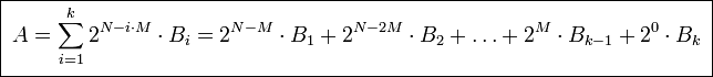
Например:
- A = F1E2D3C4B5A69788 (qword)
- A = 232 * F1E2D3C4 (dword) + 20 * B5A69788 (dword)
- A = 248 * F1E2 (word) + 232 * D3C4 (word) + 216 * B5A6 (word) + 20 * 9788 (word)
- A = 256 * F1 (byte) + 248 * E2 (byte) + … + 28 * 97 (byte) + 20 * 88 (byte)
Существуют понятия младшая часть (low) и старшая часть (hi) числа. Старшая часть входит в число с коэффициентом 2N-M, а младшая с коэффициентом 20. Например:
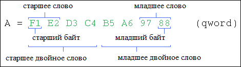
Байты числа можно хранить в памяти в различном порядке. В настоящее время используются два способа расположения: в прямом порядке байт и в обратном порядке байт. В первом случае старший байт записывается в начале, затем последовательно записываются остальные байты, вплоть до младшего. Такой способ используется в процессорах Motorola и SPARC. Во втором случае, наоборот, сначала записывает младший байт, а затем последовательно остальные байты, вплоть до старшего. Такой способ используется в процессорах архитектуры x86 и x64. Далее приведен пример:
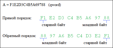
Используя подобные целочисленные типы можно представить большое количество неотрицательных чисел: от 0 до 2N-1, где N — разрядность типа. Однако, целочисленный тип подразумевает представление также и отрицательных чисел. Можно ввести отдельные типы для отрицательных чисел от -2N до -1, но тогда такие типы потеряют универсальность хранить и неотрицательные, и отрицательные числа. Поэтому для определения знака числа можно выделить один бит из двоичного представления. По соглашению, это старший бит. Остальная часть числа называется мантиссой.
Если старший бит равен нулю, то мантисса есть обычное представление числа от 0 до 2N-1-1. Если же старший бит равен 1, то число является отрицательным и мантисса представляет собой так называемый дополнительный код числа. Поясним на примере:
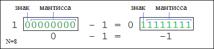
Как видно из рисунка, дополнительный код равен разнице между числом 2N-1 и модулем исходного отрицательного числа (127 (1111111) = 128 (10000000) — |-1| (0000001)). Из этого вытекает, что сумма основного и дополнительного кода одного и того же числа равна 2N-1.
Из вышеописанного получается, что можно использовать только целочисленные типы со знаком для описания чисел. Однако существует множество сущностей, которые не требуют отрицательных значений, а значит, место под знак можно включить в представление неотрицательного числа, удвоив количество различных неотрицательных значений. Как результат, в современных компьютерах используются как типы со знаком или знаковые типы, так и типы без знака или беззнаковые типы.
В итоге можно составить таблицу наиболее используемых целочисленных типов данных:
| Общее название | Название в Pascal | Название в C++ | Описание | Диапазон значений |
| unsigned byte | byte | unsigned char | беззнаковый 8 бит | 0..255 |
| signed byte | shortint | char | знаковый 8 бит | -128..127 |
| unsigned word | word | unsigned short | беззнаковый 16 бит | 0..65535 |
| signed word | smallint | short | знаковый 16 бит | -32768..32767 |
| unsigned double word | cardinal | unsigned int | беззнаковый 32 бита | 0..232-1 |
| signed double word | integer | int | знаковый 32 бита | -231..231-1 |
| unsigned quad word | uint64 | unsigned long long unsigned __int64_t (VC++) |
беззнаковый 64 бита | 0..264-1 |
| signed quad word | int64 | long long __int64_t (VC++) |
знаковый 64 бита | -263..263-1 |