
Содержание
- Add or subtract time
- Add time
- Subtract time
- Add time
- Subtract time
- How to calculate time in Excel — time difference, adding / subtracting times
- How to calculate time difference in Excel (elapsed time)
- Formula 1. Subtract one time from the other
- Formula 2. Calculating time difference with the TEXT function
- Formula 3. Count hours, minutes or seconds between two times
- Formula 4. Calculate difference in one time unit ignoring others
- Formula 5. Calculate elapsed time from a start time to now
- Formula 5. Display time difference as «XX days, XX hours, XX minutes and XX seconds»
- How to calculate and display negative times in Excel
- Method 1. Change Excel Date System to 1904 date system
- Method 2. Calculate negative time in Excel with formulas
- Adding and subtracting time in Excel
- How to add or subtract hours to time in Excel
- How to add / subtract minutes to time in Excel
- How to add / subtract seconds to a given time
- How to sum time in Excel
- How to sum over 24 hours in Excel
- Date & Time Formula Wizard — quick way to calculate times in Excel
Add or subtract time
Let’s say that you need to add two different time values together to get a total. Or, you need to subtract one time value from another to get the total time spent working on a project.
As you’ll see in the sections below, Excel makes it easy to add or subtract time.
Add time
Suppose that you want to know how many hours and minutes it will take to complete two tasks. You estimate that the first task will take 6 hours and 45 minutes and the second task will take 9 hours and 30 minutes.
Here is one way to set this up in the a worksheet.
Enter 6:45 in cell B2, and enter 9 :30 in cell B3.
In cell B4, enter =B2+B3 and then press Enter.
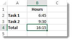
The result is 16:15—16 hours and 15 minutes—for the completion the two tasks.
Tip: You can also add up times by using the AutoSum function to sum numbers. Select cell B4, and then on the Home tab, choose AutoSum. The formula will look like this: =SUM(B2:B3). Press Enter to get the same result, 16 hours and 15 minutes.
Well, that was easy enough, but there’s an extra step if your hours add up to more than 24. You need to apply a special format to the formula result.
To add up more than 24 hours:
In cell B2 type 12:45, and in cell B3 type 15:30.
Type =B2+B3 in cell B4, and then press Enter.
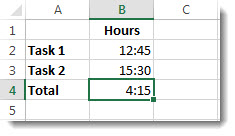
The result is 4:15, which is not what you might expect. This is because the time for Task 2 is in 24-hour time. 15:30 is the same as 3:30.
To display the time as more than 24 hours, select cell B4.
On the Home tab, in the Cells group, choose Format, and then choose Format Cells.

In the Format Cells box, choose Custom in the Category list.
In the Type box, at the top of the list of formats, type [h]:mm;@ and then choose OK.
Take note of the colon after [h] and a semicolon after mm.
The result is 28 hours and 15 minutes. The format will be in the Type list the next time you need it.
Subtract time
Here’s another example: Let’s say that you and your friends know both your start and end times at a volunteer project, and want to know how much time you spent in total.
Follow these steps to get the elapsed time—which is the difference between two times.
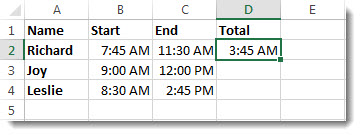
In cell B2, enter the start time and include “ a” for AM or “ p” for PM. Then press Enter.
In cell C2, enter the end time, including “ a” or “ p” as appropriate, and then press Enter.
Type the other start and end times for your friends, Joy and Leslie.
In cell D2, subtract the end time from the start time by entering the formula =C2-B2, and then press Enter.
In the Format Cells box, click Custom in the Category list.
In the Type list, click h:mm (for hours and minutes), and then click OK.
Now we see that Richard worked 3 hours and 45 minutes.
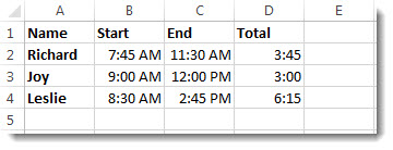
To get the results for Joy and Leslie, copy the formula by selecting cell D2 and dragging to cell D4.
The formatting in cell D2 is copied along with the formula.
To subtract time that’s more than 24 hours:
It is necessary to create a formula to subtract the difference between two times that total more than 24 hours.
Follow the steps below:
Referring to the above example, select cell B1 and drag to cell B2 so that you can apply the format to both cells at the same time.
In the Format Cells box, click Custom in the Category list.
In the Type box, at the top of the list of formats, type m/d/yyyy h:mm AM/PM.
Notice the empty space at the end of yyyy and at the end of mm.
The new format will be available when you need it in the Type list.
In cell B1, type the start date, including month/day/year and time using either “ a” or “ p” for AM and PM.
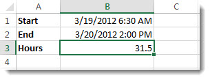
In cell B2, do the same for the end date.
In cell B3, type the formula =(B2-B1)*24.
The result is 31.5 hours.
Note: You can add and subtract more than 24 hours in Excel for the web but you cannot apply a custom number format.
Add time
Suppose you want to know how many hours and minutes it will take to complete two tasks. You estimate that the first task will take 6 hours and 45 minutes and the second task will take 9 hours and 30 minutes.
In cell B2 type 6:45, and in cell B3 type 9:30.
Type =B2+B3 in cell B4, and then press Enter.
It will take 16 hours and 15 minutes to complete the two tasks.
Tip: You can also add up times using AutoSum. Click in cell B4. Then click Home > AutoSum. The formula will look like this: =SUM(B2:B3). Press Enter to get the result, 16 hours and 15 minutes.
Subtract time
Say you and your friends know your start and end times at a volunteer project, and want to know how much time you spent. In other words, you want the elapsed time or the difference between two times.
In cell B2 type the start time, enter a space, and then type “ a” for AM or “ p” for PM, and press Enter. In cell C2, type the end time, including “ a” or “ p” as appropriate, and press Enter. Type the other start and end times for your friends Joy and Leslie.
In cell D2, subtract the end time from the start time by typing the formula: =C2-B2, and then pressing Enter. Now we see that Richard worked 3 hours and 45 minutes.
To get the results for Joy and Leslie, copy the formula by clicking in cell D2 and dragging to cell D4. The formatting in cell D2 is copied along with the formula.
Источник
How to calculate time in Excel — time difference, adding / subtracting times
 by Svetlana Cheusheva, updated on March 21, 2023
This tutorial focuses on various ways to calculate times in Excel. You will find a few useful formulas to add and subtract times, calculate time difference, or elapsed time, and more.
In the last week’s article, we had a close look at the specificities of Excel time format and capabilities of basic time functions. Today, we are going to dive deeper into Excel time calculations and you will learn a few more formulas to efficiently manipulate times in your worksheets.
How to calculate time difference in Excel (elapsed time)
To begin with, let’s see how you can quickly calculate elapsed time in Excel, i.e. find the difference between a beginning time and an ending time. And as is often the case, there is more than one formula to perform time calculations. Which one to choose depends on your dataset and exactly what result you are trying to achieve. So, let’s run through all methods, one at a time.
Add and subtract time in Excel with a special tool
No muss, no fuss, only ready-made formulas for you
Easily find difference between two dates in Excel
Get the result as a ready-made formula in years, months, weeks, or days
Calculate age in Excel on the fly
And get a custom-tailored formula
Formula 1. Subtract one time from the other
As you probably know, times in Excel are usual decimal numbers formatted to look like times. And because they are numbers, you can add and subtract times just as any other numerical values.
The simplest and most obvious Excel formula to calculate time difference is this:
Depending on you data structure, the actual time difference formula may take various shapes, for example:
| Formula | Explanation |
| =A2-B2 | Calculates the difference between the time values in cells A2 and B2. |
| =TIMEVALUE(«8:30 PM») — TIMEVALUE(«6:40 AM») | Calculates the difference between the specified times. |
| =TIME(HOUR(A2), MINUTE(A2), SECOND(A2)) — TIME(HOUR(B2), MINUTE(B2), SECOND(B2)) | Calculates the time difference between values in cells A2 and B2 ignoring the date difference, when the cells contain both the date and time values. |
Remembering that in the internal Excel system, times are represented by fractional parts of decimal numbers, you are likely to get the results similar to this:
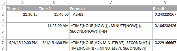
The decimals in column D are perfectly true but not very meaningful. To make them more informative, you can apply custom time formatting with one of the following codes:
| Time code | Explanation |
| h | Elapsed hours, display as 4. |
| h:mm | Elapsed hours and minutes, display as 4:10. |
| h:mm:ss | Elapsed hours, minutes and seconds, display as 4:10:20. |
To apply the custom time format, click Ctrl + 1 to open the Format Cells dialog, select Custom from the Category list and type the time codes in the Type box. Please see Creating a custom time format in Excel for the detailed steps.
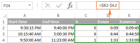
And now, let’s see how our time difference formula and time codes work in real worksheets. With Start times residing in column A and End times in column B, you can copy the following formula in columns C though E:
The elapsed time is displayed differently depending on the time format applied to the column:
Note. If the elapsed time is displayed as hash marks (#####), then either a cell with the formula is not wide enough to fit the time or the result of your time calculations is a negative value.
Formula 2. Calculating time difference with the TEXT function
Another simple technique to calculate the duration between two times in Excel is using the TEXT function:
- Calculate hours between two times:
=TEXT(B2-A2, «h»)
Return hours and minutes between 2 times:
=TEXT(B2-A2, «h:mm»)
Return hours, minutes and seconds between 2 times:
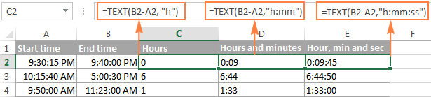
- The value returned by the TEXT function is always text. Please notice the left alignment of text values in columns C:E in the screenshot above. In certain scenarios, this might be a significant limitation because you won’t be able to use the returned «text times» in other calculations.
- If the result is a negative number, the TEXT formula returns the #VALUE! error.
Formula 3. Count hours, minutes or seconds between two times
To get the time difference in a single time unit (hours ,minutes or seconds), you can perform the following calculations.
Calculate hours between two times:
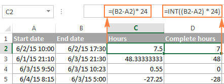
To present the difference between two times as a decimal number, use this formula:
Supposing that your start time is in A2 and end time in B2, you can use a simple equation B2-A2 to calculate the difference between two times, and then multiply it by 24, which is the number of hours in one day:
To get the number of complete hours, use the INT function to round the result down to the nearest integer:
Total minutes between two times:
To calculate the minutes between two times, multiply the time difference by 1440, which is the number of minutes in one day (24 hours * 60 minutes = 1440).
As demonstrated in the following screenshot, the formula can return both positive and negative values, the latter occur when the end time is less than the start time, like in row 5:

Total seconds between times:
To get the total seconds between two times, you multiply the time difference by 86400, which is the number of seconds in one day (24 hours * 60 minutes * 60 seconds = 86400).
In our example, the formula is as follows:
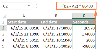
Note. For the results to display correctly, the General format should be applied to the cells with your time difference formula.
Formula 4. Calculate difference in one time unit ignoring others
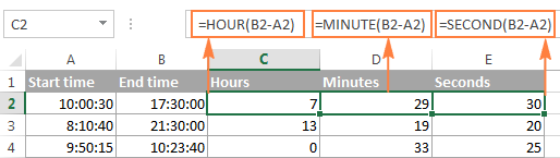
To find the difference between 2 times in a certain time unit, ignoring the others, use one of the following functions.
- Difference in hours, ignoring minutes and seconds:
=HOUR(B2-A2)
Difference in minutes, ignoring hours and seconds:
=MINUTE(B2-A2)
Difference in seconds, ignoring hours and minutes:
When using Excel’s HOUR, MINUTE and SECOND functions, please remember that the result cannot exceed 24 for hours and 60 for minutes and seconds.
Note. If the end time is less than the start time (i.e. the result of the formula is a negative number), the #NUM! error is returned.
Formula 5. Calculate elapsed time from a start time to now
In order to calculate how much time has elapsed since the start time to now, you simply use the NOW function to return today’s date and the current time, and then subtract the start date and time from it.
Supposing that the beginning date and time is in call A2, the formula below returns the following results, provided you’ve applied an appropriate time format to column B, h:mm in this example:

In case the elapsed time exceeds 24 hours, use one of these time formats, for example d «days» h:mm:ss like in the following screenshot:

If your starting points contain only time values without dates, you need to use the TIME function to calculate the elapsed time correctly. For example, the following formula returns the time elapsed since the time value in cell A2 up to now:
=TIME(HOUR(NOW()), MINUTE(NOW()), SECOND(NOW())) — A2
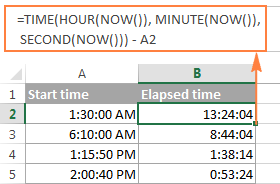
Note. The elapsed time is not updated in real-time, it refreshes only when the workbook is reopened or recalculated. To force the formula to update, press either Shift + F9 to recalculate the active spreadsheet or hit F9 to recalculate all open workbooks.
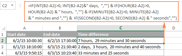
Formula 5. Display time difference as «XX days, XX hours, XX minutes and XX seconds»
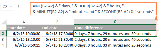
This is probably the most user-friendly formula to calculate time difference in Excel. You use the HOUR, MINUTE and SECOND functions to return corresponding time units and the INT function to compute the difference in days. And then, you concatenate all these functions in a single formula along with the text labels:
=INT(B2-A2) & » days, » & HOUR(B2-A2) & » hours, » & MINUTE(B2-A2) & » minutes and » & SECOND(B2-A2) & » seconds»
To instruct your Excel time difference formula to hide zero values, embed four IF functions into it:
=IF(INT(B2-A2)>0, INT(B2-A2) & » days, «,»») & IF(HOUR(B2-A2)>0, HOUR(B2-A2) & » hours, «,»») & IF(MINUTE(B2-A2)>0, MINUTE(B2-A2) & » minutes and «,»») & IF(SECOND(B2-A2)>0, SECOND(B2-A2) & » seconds»,»»)
The syntax may seem excessively complicated, but it works 🙂
Alternatively, you can calculate time difference by simply subtracting the start time from the end time (e.g. =B2-A2 ), and then apply the following time format to the cell:
d «days,» h «hours,» m «minutes and» s «seconds»
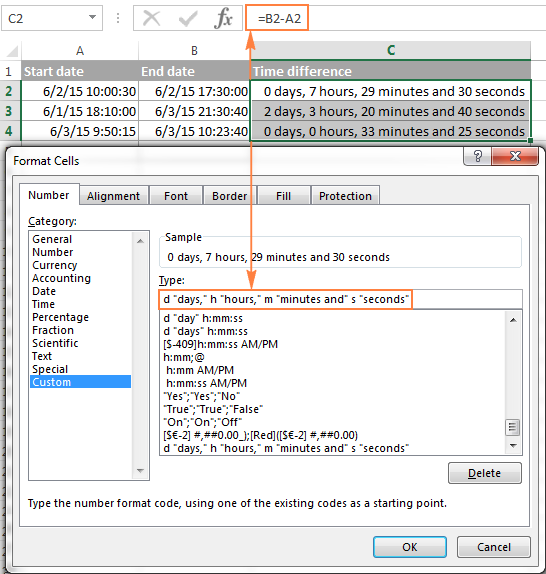
An advantage of this approach is that your result would be a normal time value that you could use in other time calculations, while the result of the complex formula discussed above is a text value. A drawback is that the custom time format cannot distinguish between zero and non-zero values and ignore the latter. To display the result in other formats, please see How to show time over 24 hours, 60 minutes, 60 seconds.
How to calculate and display negative times in Excel
When calculating the time difference in Excel, you may sometimes get the result as ###### error because the difference is a negative time. But is there a way to show negative times properly in Excel? Of course, there is a way, and even more than one 🙂
Method 1. Change Excel Date System to 1904 date system
The fastest and easiest way to display negative time normally (with a minus sign) is switching to the 1904 date system. To do this, click File > Options > Advanced, scroll down to the When calculating this workbook section and put a tick in the Use 1904 date system box.

Click OK to save the new settings, and from now on negative times will be displayed correctly, like negative numbers:

Method 2. Calculate negative time in Excel with formulas
Is changing Excel’s default Date System is not an option, then you can force negative times to display properly using one of the following formulas:
=IF(A2-B2>0, A2-B2, «-» & TEXT(ABS(A2-B2),»h:mm»))
=IF(A2-B2>0, A2-B2, TEXT(ABS(A2-B2),»-h:mm»))
Both formulas check if the time difference (A2-B2) is greater than 0, and if it is they return that difference. If the time difference is less than zero, the first formula calculates the absolute difference and concatenates the minus sign. The second formula yields exactly the same result by using a negative time format «-h::mm«.

Note. Please keep in mind that unlike the first method that treats negative times as negative numeric values, the result of the TEXT function is always a text string that cannot be used in calculations or other formulas.
Adding and subtracting time in Excel
Basically, there are 2 ways to add and subtract time in Excel:
- Using the TIME function
- Using arithmetic calculations based on the number of hours (24), minutes (1440) and seconds (86400) in one day
The TIME(hour, minute, second) function makes Excel time calculations really easy, however it does not allow adding or subtracting more than 23 hours, or 59 minutes, or 59 seconds. If you are working with bigger time intervals, then use one of the arithmetic calculations demonstrated below.
How to add or subtract hours to time in Excel
To add hours to a given time in Excel, you can use one the following formulas.
TIME function to add under 24 hours
For example, if your start time is in cell A2, and you want to add 2 hours to it, the formula is as follows:
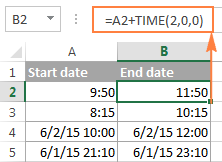
Note. If you try adding more than 23 hours with the TIME function, the specified hours will be divided by 24 and the remainder will be added to the start time value. For example, if you try to add 25 hours to «6/2/2015 10:00 AM» (cell A4) using the formula =A4 + TIME(25, 0, 0) , the result will be «06/02/2015 11:00», i.e. A4 + 1 hour.
Formula to add any number of hours (under or over 24 hours)
The following formula has no limitations to the number of hours you want to add:
For example, to add 28 hours to the start time in cell A2, enter the following formula:

To subtract hours from a given time, you use analogous formulas, and just replace «+» with the minus sign:
For example, to subtract 3 hours from the time in cell A2, either of the following formulas will do:
To subtract more than 23 hours, use the first one.
How to add / subtract minutes to time in Excel
To add minutes to a given time, employ the same techniques that we’ve just used for adding hours.
To add or subtract under 60 minutes
Use the TIME function and supply the minutes you want to add or subtract in the second argument:
And here are a couple of real-life formulas to calculate minutes in Excel:
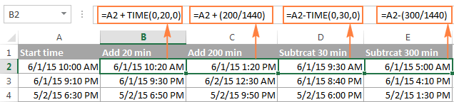
To add 20 minutes to the time in A2: =A2 + TIME(0,20,0)
To subtract 30 minutes from the time in A2: =A2 — TIME(0,30,0)
To add or subtract over 60 minutes
In your calculation, divide the number of minutes by 1440, which is the number of minutes in a day, and add the quotient to the start time:
To subtract minutes from time, simply replace plus with the minus sign. For example:
To add 200 minutes: =A2 + (200/1440)
To subtract 300 minutes: =A2 -(300/1440)
How to add / subtract seconds to a given time
Second calculations in Excel are done in a similar fashion.
To add under 60 seconds to a given time, you can use the TIME function:
To add more than 59 seconds, use the following formula:
To subtract seconds, utilize the same formulas with the minus sign (-) instead of plus (+).
In your Excel worksheets, the formulas may look similar to these:
To add 30 seconds to A2: =A2 + TIME(0,0,31)
To add 1200 seconds to A2: =A2 + (1200/86400)
To subtract 40 seconds from A2: =A2 — TIME(0,0,40)
To subtract 900 seconds from A2: =A2 — (900/86400)
How to sum time in Excel
The Excel sum time formula is the usual SUM function, and applying the proper time format to the result is what does the trick.
Supposing you have a few project times in column B and you want to add them up. You write a simple SUM formula like the one below and get the result in the default format such as hh:mm:ss.
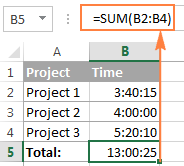
In some cases the default time format works just fine, but sometimes you may want more, for example to display the total time as minutes and seconds, or seconds only. The good news is that no other calculations are required, all you have to do is apply custom time format to the cell with the SUM formula.
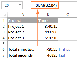
Right click the cell and select Format Cells in the context menu, or press Ctrl + 1 to open the Format Cells dialog box. Select Custom from the Category list and type one of the following time formats in the Type box:
- To display total time as minutes and seconds: [m]:ss
- To display total time as seconds: [ss]
The result will look as follows:
How to sum over 24 hours in Excel
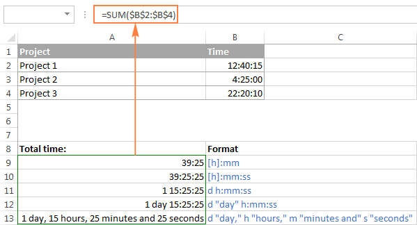
In order to add up more than 24 hours, you use the same SUM formula as discussed above, and apply one of the following time formats to the cell:
| Format | Displays as | Explanation |
| [h]:mm | 30:10 | Hours and minutes |
| [h]:mm:ss | 30:10:20 | Hours, minutes and seconds |
| [h] «hours», mm «minutes», ss «seconds» | 30 hours, 10 minutes, 20 seconds | |
| d h:mm:ss | 1 06:10:20 | Days, hours, minutes and seconds |
| d «day» h:mm:ss | 1 day 06:10:20 | |
| d «day,» h «hours,» m «minutes and» s «seconds» | 1 day, 6 hours, 10 minutes and 20 seconds |
To see how these custom time formats may look like in your Excel worksheet, please have a look at the screenshot below, where the same SUM formula is entered in cells A9 to A13:
Note. The above custom time formats work for positive values only. If the result of your time calculations is a negative number, e.g. when you are subtracting a bigger time from a smaller time, the result will be displayed as #####. To display negative times differently, please see custom format for negative time values.
Also, please keep in mind that the time format applied to a cell changes only the display presentation without changing the cell’s value. For example, in the screenshot above, cell A13 looks like text, but in fact it’s a usual time value, which is stored as a decimal in the internal Excel system. Meaning, you are free to refer to that cell in other formulas and calculations.
Date & Time Formula Wizard — quick way to calculate times in Excel
Now that you know a bunch of different formulas to add and subtract times in Excel, let me show you the tool that can do it all. Okay, almost all 🙂
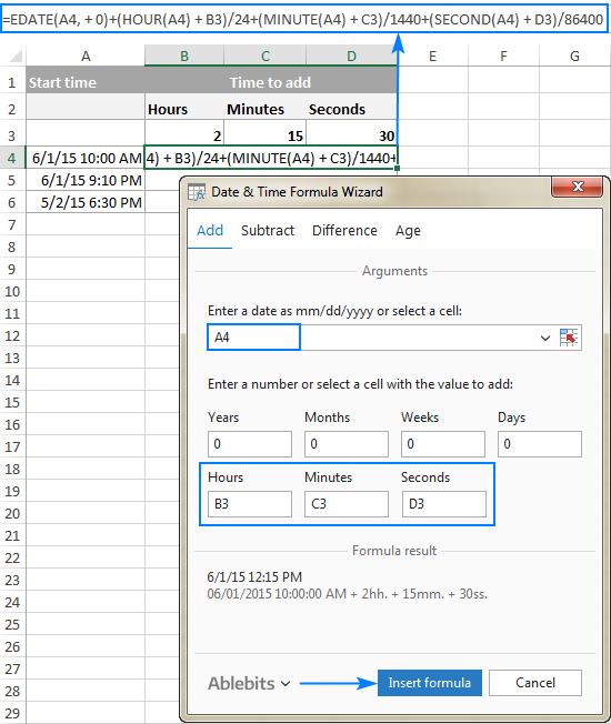
Here comes Ablebit’s Date & Time Formula Wizard for Excel:

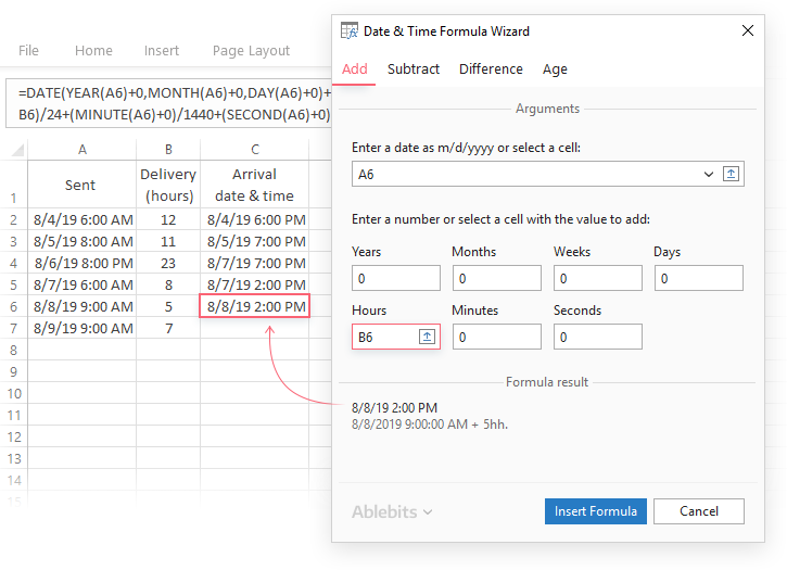
In the Date & Time Wizard dialog window, you switch to the Add or Subtract tab, depending on which operation you want to perform, and do the following:
- Click the Show time fields link in the left part of the window.
- Supply values or cell references for the formula arguments. As you fill in the argument boxes, the wizard builds the formula in the selected cell.
- When finished, click the Insert Formula
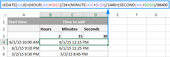
That’s it! For example, this is how you can add the specified number of hours, minutes and seconds to the time in A4:
If you need to copy the formula to other cells, fix all references except the cell containing the original time (A4) with the $ sign like shown in the screenshot below (by default, the wizard always uses relative references). Then double-click the fill handle to copy the formula down the column and you are good to go!
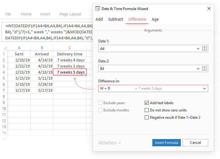
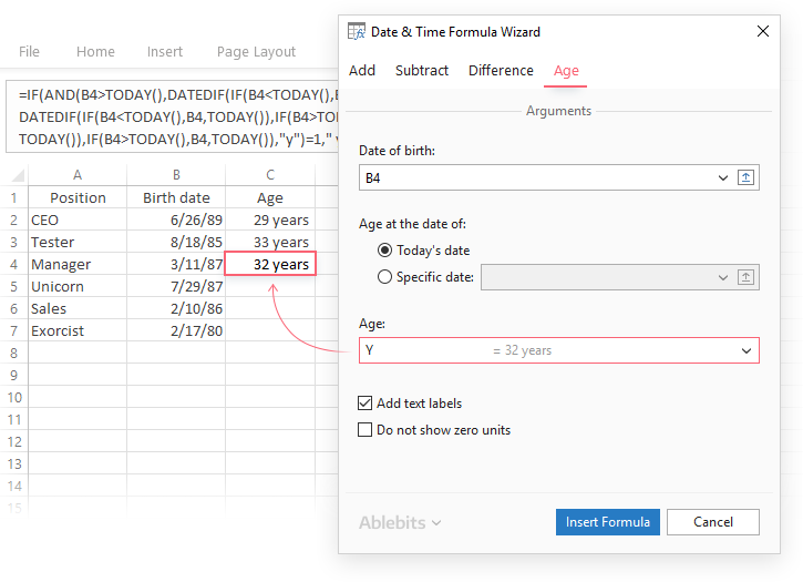
Besides time calculations, the wizard can also add and subtract dates, get the difference between two dates, and calculate age from the birthdate.
If you are curious to try this tool in your own worksheets, you are welcome to download the evaluation version of our Ultimate Suite below.
This is how you calculate time in Excel worksheets. To learn other ways to manipulate dates and times in Excel, I encourage you to check out the resources at the end of this article. I thank you for reading and hope to see you on our blog next week!
Источник

on
March 11, 2019, 3:32 AM PDT
Use Excel to calculate the hours worked for any shift
With Microsoft Excel, you can create a worksheet that figures the hours worked for any shift. Follow these step-by-step instructions.
We may be compensated by vendors who appear on this page through methods such as affiliate links or sponsored partnerships. This may influence how and where their products appear on our site, but vendors cannot pay to influence the content of our reviews. For more info, visit our Terms of Use page.
To calculate in Excel how many hours someone has worked, you can often subtract the start time from the end time to get the difference. But if the work shift spans noon or midnight, simple subtraction won’t cut it.
However, you can easily create an Excel worksheet that correctly figures the hours worked for any shift.
LEARN MORE: Office 365 Consumer pricing and features
Follow these steps:
- In A1, enter Time In.
- In B1, enter Time Out.
- In C1, enter Hours Worked.
- Select A2 and B2, and press [Ctrl]1 to open the Format Cells dialog box.
- On the Number tab, select Time from the Category list box, choose 1:30 PM from the Type list box, and click OK.
- Right-click C2, and select Format Cells.
- On the Number tab, select Time from the Category list box, choose 13:30 from the Type list box, and click OK.
- In C2, enter the following formula:
=IF(B2<A2,B2+1,B2)-A2
If you enter 11:00 PM as the Time In and enter 7:00 AM as the Time Out, Excel will display 8, the correct number of hours worked.
A bonus Microsoft Excel tip
From the article 10 things you should never do in Excel by Susan Harkins:
Rely on multiple links: Links between two workbooks are common and useful. But multiple links where values in workbook1 depend on values in workbook2, which links to workbook3, and so on, are hard to manage and unstable. Users forget to close files, and sometimes they even move them. If you’re the only person working with those linked workbooks, you might not run into trouble, but if other users are reviewing and modifying them, you’re asking for trouble. If you truly need that much linking, you might consider a new design.
This bonus Excel tip is also available in the free PDF 30 things you should never do in Microsoft Office.
Editor’s note on March 11, 2019: This Excel article was first published in June 2005. Since then, we have included a video tutorial, added a bonus tip, and updated the related resources.
Also See
-
How to add a drop-down list to an Excel cell
(TechRepublic) -
Tap into the power of Excel’s data validation feature (free PDF)
(TechRepublic) -
You’ve been using Excel wrong all along (and that’s OK)
(ZDNet) -
A cheatsheet of Excel shortcuts that make inserting data faster
(TechRepublic) -
Six clicks: Excel power tips to make you an instant expert
(ZDNet) -
10 things you should never do in Excel
(TechRepublic)
-
Microsoft
-
Software
Time In And Time Out — Excel |
|
I have a spreadsheet which captures data from a magnetic card reader when the user swipes their ID card. I want to capture attendance and how long the user is at an event, so I want them to swipe in when they arrive and swipe out when they leave.
Each swipe calls the worksheet_change function which runs a macro and writes the users id number in column B and the users name in column C and the time of the swipe in column D.
What I need to do is to check column B for the ID, if it’s found then it means the user is leaving and I want to write the time of the swipe in column E of the row where the user ID exists. If the ID isn’t found in column B then the user id, name and time of swipe needs to be written in columns B, C, D of the first empty row. The raw data is written to column A first empty cell each time a card is swiped.
Thanks
![]()
Excel VBA Course — From Beginner to Expert
200+ Video Lessons
50+ Hours of Instruction
200+ Excel Guides
Become a master of VBA and Macros in Excel and learn how to automate all of your tasks in Excel with this online course. (No VBA experience required.)
(80% Discount Ends Soon!)
View Course
Similar Topics
I have an excel 2007 file sitting in a shared network folder. I only want one user to be able to make changes at a time (any other users would get a read-only). For some reason it currently does not do this, and I have multiple users with the same doc open. I’m concerned that changes will get over-written when 2 people are saving their changes. Can anyone help me with the settings for this.

Good day… I need an IF Function that will allow me to action a time in a time range:
… If the time 04:16 falls in the time range 04:00 — 04:29, than put a one (1) in the filed x…
… If the time 04:16 doesn’t fall in the time range 04:00 — 04:29, than leave the x fiel empty
Any help is appreciated.
Hi everyone,
I found an excellent macro this morning that allows the user to filter a pivot table based on the value found in a specific cell. This cell essentially acts as a search bar, allowing the user to type in what they are looking for rather than select it from a drop-down list.
The macro works perfectly for my purposes except in one regard: I can no longer perform a «show all» filter. If I leave the «search bar» cell blank, the pivot table shows nothing. I’m sure that there is an easy fix for this but I’m still learning the basics of how to write and use macros. How can I change the code so that when I leave the cell blank, the pivot table shows all? The search bar cell is D2.
Thanks for your time!
Sorry for the question. Normally I find answers to my excel questions by going through the help tab or by searching on Google. However, I don’t even know what question to ask on this one!?!
Basically I have created a spreadsheet with several columns, but I have one column that lists the shirt size (YS, YM, YL, AS, AM, AL, XL, 2X, 3X) of each person. Is there a formula that I can create that will tabulate the number of sizes (i.e. AS=2, AM=7, etc.)?
In previous years I made a column for each size, and simply placed a «1» in the correct column, and had excel just add the 1’s from each column. However, that takes more time and space. I was hoping to streamline it this time around.
Thanks for taking the time to read this post. Any help would be appreciated! Thanks, doug
I have a VBMacro Excel file loaded on a Server that numerous people access. A Macro in this file creates a Copy of a specific Sheet within the Active Workbook and I want to Save it to the individual’s Desktop.
How do I find out what the current User’s desktop folder path is each time the Marco is run by a different User?
Example User’s path: ‘C:Documents and SettingsjfarcDesktop’
Where ‘jfarc’ is the name of the current User which, will of course change with every different User that runs the Macro.
Also, is there a way to pull out of Excel what is the current User’s ‘Options | General | Default File Location’ entry? Which may differ from the above directory.
I am familiar with and use the following coding for Opening/Saving files to the current directory of the opened workbook, but it only gives the path of the existing Excel workbook and not the current User’s Directory Path:
Dim wbThis As Workbook
Set wbThis = ThisWorkbook
ChDir wbThis.Path
Hi there
I am trying to calculate our On Time Delivery. I want this as a simple percentage of jobs. I have got this running in the following way:
Column M — Estimated Delivery dates
Column N — Actual Delivery dates
Column O — =IF(SUM(M2-N2)>0,1,0)
Then I have calculated On Time Delivery as: =SUM((SUM(O2:O252))/(COUNTA(N2:N252)))
This seems to work fine. My problem is, if we enter a date in Estimated without a corresponding Actual date, the formula for Column O fills out anyway and improves our On Time Delivery Percentage. How can I set this up so that the formula doesn’t calculate if there is no data in Column N?
Any help much appreciated
Thanks,
James
Hi,
I made a simple worksheet that we have been manually entering the time for employees, but there are too many errors (even with simple math). Can someone help me convert the time of ex: written 8-4:30 or 10-3 (meaning 8:00am to 4:30pm) where you have the total weekly hours? Right now I have a column for overtime. Is there a way to automatically calculate the over time also? The work day is 8-4:30 with a half hour lunch (lunch is not calculated into the hours, so you minus a half hour). 8-4:30 equals 8 hours. So, if a person works 8am to 6:30pm, how can I set it up where in the first row of time, I will type in 8-6:30pm. In the totals column to the far right, it will display 8 hours. In the (O.T.) column, it will display 2 hours.
This way, when I call in my payroll, I will have the total «regular» hours in one row and underneath, I will have the total overtime hours.
Or… does anyone have a better solution to keeping track of their hours?
Thanks!
Marty
I have never really used VBA and so am completely stuck at this problem. I need to create a macro which auto-populates a master worksheet from the individual user sheets in a shared workbook.
Sheet 1 is the master sheet «Team Stats». There will be an undetermined number of individual worksheets to accomodate new staff.
Each worksheet will be identical, using columns A-I with row 1 having the headings:
Date, Name, Reference, Value, Price, Age, Purchased?, Destination, Add. Products (the last 3 columns will have a drop-down list which will be used to enter data into the cell).
There will be a varying number of rows in each of the individual sheets.
If possible I would like the macro to run every time data is entered into one of the individual worksheets. If this is not then it would be fien to update every time the workbook is opened.
If anyone can help it would really cut down the time I spend collating these stats every day!
Hello,
I have two columns of data: column A contains the date and time in the form dd/mm/yyyy. Column B contains a number value. All the times are in order, so column A looks like:
01/01/2007
02/01/2007
03/01/2007
I have data from 2007 to 2010. I need to calculate an average daily value (in column B) for each month, and display it in column C. So, for January, I need to calculate the average of 31 days, February, 28 days, etc.
Is there a function I can use to do this? I’ve been trying the AVERAGEIF formula but can’t get it to work. Any ideas would be much appreciated!
Many thanks,
Caitlin
I have a workbook that has compliance dates in columns «F»,»G» and «H» from row 7. What I need is when the date in either column comes within 30 days to auto send an email, address in column «A», recipients name in column «B». and then place todays date in column ‘P». ALso need to send a follow up email when either date comes within 7days and then place todays date in column «Q». If there is a date in column «P» then don’t send email. If there is a date in column «Q» then don’t send follow up. Can this be done without the users intervention and each time the workbook is opened.
Thanks in advance for any assistance.
Mick
Happy Day to all,
Can you please help me,
A1= time in
B1= time out
C1= time in
D1= time out
I want to calculate the late and under time,
Office start at 9:am w/30 mins Grace period,
The break time is one hour only, please include over breaktime in calculation.
End of office hours 6:00 pm, strickly no over time
I use a excel file through the course of the day and need to insert the current date in one column and the current time in the next column. I want to be able to just highlight the selected range of cells I need to insert into and hit a macro button and have the date and time inserted into just the cells I have highlighted. I’m not sure how to make this work with just the cells I’ve highlighted. Any help any one can give me would be greatly appreciated. Thanks!
Mike
Thought I’d start this topic since there seem to be a number of topics where the answer seems to be to use one of the above rather than other. Thought I’d kick off with my 2 cents’ worth.
I have a userform with frames containing textboxes. The user enters a currency value and once they leave the control, then a protected textbox next to it shows the corresponding value in SEK. I started off using the exit event but ran into 2 problems.
If you tabbed out of the last textbox in the frame, the exit event never kicked in (this is documented in other topics but took some time to find). This resulted in me using the exit event for all except the last textbox in the frame that used afterupdate instead
I then discovered that the exit events didn’t kick in if, instead of tabbing out of the field, I deliberately placed focus in a control elsewhere on the form. Changing the event from exit to afterupdate corrected this.
My question then is … could you guys document in this topic when you would/must use the exit rather than the afterupdate event (or vice-versa).
Thanks
I am looking for assistance in having one cell in a text format equals another cell that contains a time value in hh:mm format.
For example: Cell A1 has a time format (hh:mm) value of 04:00; which is the Start Time. I would like cell D1 to have a text format value of «04:00» (result is dependant upon what is entered in A1). I would duplicate the same formulas to reflect Stop Times in other cells.
My final result is to have another cell (F1) use the Concatenate formula to have the Start and Stop time shown in one cell as «04:00 — 12:30». The times would change based on the Time formated values entered into the Start and Stop time cells.
I have researched this in the board and found many excellent ways to do the opposite, but not convert Time format to Text format. Any assistance is greatly appreciated.
-Shane
Hey there,
I have been tasked with introducing userforms into an excel sheet and tbh I’m quite amazed that excel has this capability of adding userforms to excel sheets.
Anyway, I have 2 columns of data in an excel sheet and I wish to add this to a userform so that the userform displays the 2 columns beside each other with headings, like a table. The user should then be able to select a particular row and insert it into the specified cell.
I would also like the user to select a row on the table and then be able to bring up another table depending on the row selected…basically so that the user can draw deeper into the information that they require.
I have an example excel sheet where I have 2 sheets. One sheet is the user entry sheet called User Entry Screen. the next sheet is the tables sheet where my tables are held. Once the user selects the cell shown in the example sheet, it should then bring up the user form. the user then, depending on which item clicked, then gets shown the next window with a table and info on it. then user should then be able to select an item and the cells on the user entry screen would then get populated.
Personally I think this is a really tricky challenge and any help with doing this would be extremely appreciated.
I’ll post up further comments as I am trying to work my way through it!
Thanks,
Jag
Entering time values in custom format [h]:mm:ss
Cells accept hours over 23,
Adding cells in column returns correct total time.
Have not found a way to multiply these cells by a $ hourly rate.
So use HOUR(cell ref) and MINUTE(cell ref) to capture values in referenced
cell — then use these values to calculate total payment for $rate per hour.
However, the HOUR(cell ref) formula returns the hours in excess of 24 when
the cell contains an hour value in excess of 23 (ie 27 hours returns 3).
Hello,
i’ve got the following problem:
I want users to double-click on a row on a protected sheet and then do some code based on the row-number of the clicked cell. I’ve protected the sheet because it contains a lot of formula’s.
When a user double-clicks a row it triggers the code through the Workbook_SheetBeforeDoubleClick event.
After the code is executed Excel shows a message that the cell that was clicked was protected etc etc.
How can I prevent this message from popping up?
I’ve already tried
Code:
application.displaywarnings = false
but that didn’t work
Thanks
In Excel I have been trying to find an easier way to calculate a time
difference where the times cross midnight. Example:
Start time: 23:50:00
End time: 00:15:00
How would you formulate an equation to determine the duration of time or
differnce between the start and end time?
Hi all,
I have a dillemma here,
I have to create a schedule which incorporates lunches automatically (either half hour or 1-hour lunches, depending on the circumstances).
The schedule only has time in and time out, but I need excel to automatically deduct the lunch break depending on the circumstance:
If you worked less than 6 hours = no lunch
If you worked more than 6 hours, but less than or equal to 8 hours = 0.5 hour lunch
If you worked more than 8 hours = 1 hour lunch
I am assuming the formula for this will be really long, but I have looked online everywhere and have not found ONE formula for it. I can’t put lunch breaks seperately, so all I have to work with is Time in/out.
Also, I wouldn’t be able to use military time, so I don’t know how excel can assume that time in is in the morning, and time out is in teh evening and/or half-day.
If someone can help it would be greatlyyyy appreciated
Helllo,
I have written a macro and at the end it displays a message «The macro has finished».
I would like this message box to disappear after 2 seconds automatically so that users don’t have to press the OK button all the time.
can this happen ?
thanks
andy
This free monthly time-in time-out timesheet helps in tracking employee hours within 4 weeks. It is downloadable and printable in Excel format.
This monthly time in time out timesheet template is a free downloadable tool that can be used to track working hours of employees in a 4-week basis. It allows employees to enter their clock in and clock out details.
The monthly timesheet is designed with four separate tables, giving you clear details on the employee’s total work hours every week. It has simple features, so you can easily edit or customize it. It’s printable, editable, and downloadable in Excel format.
This monthly timesheet template excel features formulas, allowing automatic calculations for the weekly total and monthly total of employee work hours based upon the daily time entry. These formulas are the main reason why this template is convenient to use.
Moreover, this template considers lunch unpaid, therefore, you can leave this column blank, or if preferred, you can enter the number of minutes or hours (e.g., 1 hour). Whether or not you input your lunch hours will not affect the calculations of this timesheet.
Use this monthly timesheet template and start keeping organize records of your employee’s work hours. To use, just fill out details on the blank sections provided. It includes sections for company name, employee name, employee ID, start date, end date, date, day of week, time in, time out, lunch, total hours, and weekly total. The lowermost part also displays a field where the manager can attach his/her signature upon approval of the timesheet.
Instructions in using the Timesheet:
-
Enter company name and employee details.
-
Enter start date and end date of the work week.
Once start date is entered, the remaining dates for the four-week period will be automatically generated, along with the specific day of the week. -
Enter time in and time out details for each day in a sample format of 8 am or 8:30 am.
When entering the time in and time out in Excel timesheet, make sure you put a space between the time and the word AM/PM for the formulas to work. Example format: 8 am, 1:30 pm. -
If preferred, enter lunch time.
Enter lunch time under lunch column only if desired. Entering this data will not affect the calculation as this timesheet considers lunch unpaid. However, if you want to add these figures, feel free to do so. You can input the lunch duration using this format (e.g., 1 hour). -
Review, email, or print the completed timesheet.
Maintenance Alert: Saturday, April 15th, 7:00pm-9:00pm CT. During this time, the shopping cart and information requests will be unavailable.
Categories: Advanced Excel
Working with time in Excel can be a problem. Have you ever calculated how long a person was at work, and then wanted to multiply that time by an hourly wage? It isn’t difficult to fail miserably! But, if you know the trick, Excel time formulas are easy.
First, start with formatting.
- Columns A and B (employee’s Time In and Time Out) can be formatted to Time, AM/PM.
- Column C (Hours Worked) should be formatted to Time, Military. This omits the AM PM markers and creates a true figure to reflect the amount of time passed. You need a true reflection of time passed in order to work with totals accurately.
- Column D (Hours) should be formatted as a number with two decimal places.
Columns E and F should be formatted to Currency or Accounting, your choice.
Now that your formatting is set, let’s get into Excel time formula logic.
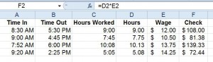
Column C contains a formula as shown in Illustration 1, =B2-A2. This calculates the number of hours the employee worked.
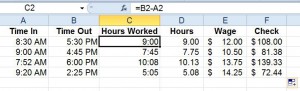
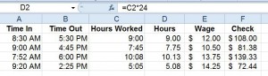
Column D, as mentioned, is formatted to a number, with two decimals. It contains the formula =C2*24. This time formula is so important because of how Excel is set up. Excel stores time values as decimal fractions of a 24 hour day. One hour equals 1/24th of a day. Thus, to get a whole number, you can use in calculation, you must multiply the value in column C by 24. Think of it like this. With a time like 7:30, C2 would equal 7.50, which is the number equivalent to seven hours and thirty minutes. See Illustration 2.
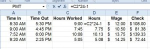
What if your employees have a lunch hour? You can set up your time formula to subtract 1. See Illustration 3.
Now that your formatting and time formulas are properly considered and applied, you can multiply Column D by Column E to reach the final paycheck total.
Working with time in and out of Excel, can include troublesome conversions. Using Excel with the tips listed can save a great deal of time and a few headaches as well. Next time you are adding or multiplying hours and minutes, consider using an Excel time formula.
PRYOR+ 7-DAYS OF FREE TRAINING
Courses in Customer Service, Excel, HR, Leadership,
OSHA and more. No credit card. No commitment. Individuals and teams.