
In this post, we’re going to learn everything there is to know about Excel Tables!
Yes, I mean everything and there’s a lot.
This post will tell you about all the awesome features Excel Tables have and why you should start using them.
What is an Excel Table?
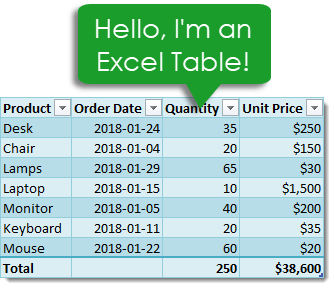
Excel Tables are containers for your data.
Imagine a house without any closets or cupboards to store your things, it would be chaos! Excel tables are like closets and cupboards for your data, they help to contain and organize data in your spreadsheets.
In your house, you might put all your plates into one kitchen cupboard. Similarly, you might put all your customer data into one Excel table.
Tables tell excel that all the data is related. Without a table, the only thing relating the data is proximity to each other.
Ok, so what’s so great about Excel Tables other than being a container to organize data? A lot actually. This post will tell you about all the awesome features tables have and should convince you to start using them.
Video Tutorial
The Parts of a Table
Throughout this post, I’ll be referring to various parts of a table, so it’s probably a good idea that we’re both talking about the same thing.
This is the Column Header Row. It is the first row in a table and contains the column headings that identify each column of data. Column headings must be unique in the table, they cannot be blank and they cannot contain formulas.
This is the Body of the table. The body is where all the data and formulas live.
This is a Row in the table. The body of a table can contain one or more rows and if you try to delete all the rows in a table a single blank row will remain.
This is a Column in the table. A table must contain at least one column.
This is the Total Row of the table. By default, tables don’t include a total row but this feature can be enabled if desired. If it’s enabled, it will be the last row of the table. This row can contain text, formula or remain blank. Each cell in the total row will have a drop down menu that allows selection of various summary formula.
Create a Table from the Ribbon
Creating an Excel Table is really easy. Select any cell inside your data and Excel will guess the range of your data when creating the table. You’ll be able to confirm this range later on. Instead of letting Excel guess the range you can also select the entire range of data in this step.
With the active cell inside your data range, go to the Insert tab in the ribbon and press the Table button found in the Tables section.
The Create Table dialog box will pop up. Excel guesses the range and you can adjust this range if needed using the range selector icon on the right hand side of the Where is the data for your table? input field. You can also adjust this range by manually typing over the range in the input field.
Checking the My table has headers box will tell Excel the first row of data contains the column headers in your table. If this is unchecked Excel will create generic column headers for the table labelled Column 1, Column 2 etc…
Press the Ok button when you’re satisfied with the data range and table headers check box.
Congratulations! You now have an Excel table and your data should look something like the above depending on the default style of your tables.
Contextual Table Tools Design Tab
Whenever you select a cell inside a table, you will notice a new tab appear in the ribbon labelled Table Tools Design. This is a contextual tab and only appears when a table is selected. When the active cell moves outside the table, the tab will disappear again.
This is where all the commands and options related to tables will live. This is where you’ll be able to name your table, find table related tools, enable or disable table elements and change your table’s style.
Create a Table with a Keyboard Shortcut
You can also create a table using a keyboard shortcut. The process is the same as described above but instead of using the Table button in the ribbon you can press Ctrl + T on your keyboard. It’s easy to remember since T is for Table!
There is actually another keyboard shortcut that you can use to create tables, Ctrl + L will also do the same thing. This is a legacy from when tables were called lists (L is for List).
Name a Table
Anytime you create a new table Excel will give it an initial generic name starting with Table1 and increasing sequentially. You should always rename your table with a descriptive and short name.
Not all names are allowed. There are a few rules for a table name.
- Each table must have a unique name within a workbook.
- You can only use letters, numbers and the underscore character in a table name. No spaces or other special characters are allowed.
- A table name must begin with either a letter or an underscore, it can not begin with a number.
- A table name can have a maximum of 255 characters.
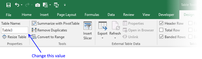
Select any cell inside your table and the contextual Table Tools Design tab will appear in the ribbon. Inside this tab you can find the Table Name under the Properties section. Type over the generic name with your new name and press the Enter button when finished to confirm the new name.
Rename a Table
Renaming a table you’ve already named is the same process as naming a table for the first time. If you think about it, when you first name a table you’re actually renaming it from the generic name of Table1 to a new name.
So go back to the Table Tools Design tab and type your new name over the old one in the Table Name and press Enter. Easy, and the name is changed.
Changing your table name this way requires navigating to your table and selecting a cell within it, so it can be tedious if you need to rename a lot of tables across different sheets in your workbook. Instead, you can change any of your table names without going to each table using the Name Manager.
Go to the Formula tab and press the Name Manager button in the Defined Names section. You’ll be able to see all your named objects here. The table objects will have a small table icon to the left of the name. You can filter to show only the table objects using the Filter button in the upper right hand corner and selecting Table Names from the options.
You can then edit any name by selecting the item and pressing the Edit button. You’ll be able to change the name and add some comments to describe the data in your table.
Navigate Tables with the Name Box
You can easily navigate to any table in your workbook using the name box the the left of the formula bar. Click on the small arrow on the right side of the name box and you will see all table names in the workbook listed. Click on any of the tables listed and you will be taken to that table.
Convert a Table Back to a Normal Range
Ok, you changed your mind and don’t want your data inside a table anymore. How do you convert it back into a regular range?
If changing it to a table was the last thing you did, Ctrl + Z to undo your last action is probably the quickest way.
If it wasn’t the last thing you did, then you’re going to need to use the Convert to Range command found in the Table Tools Design tab under the Tools section.
You’ll be prompted to confirm that you really want to convert the table to a normal range. Noooooo, don’t do it, tables are awesome!
If you click on yes, then all the awesome benefits from tables will be gone except for the formatting design. You’ll need to manually clear this from the range if you want to get rid it. You can do this by going to the Home tab then pressing the Clear button found in the Editing section, then selecting Clear Formats.
This can also be done from the right click menu. Right click anywhere in the table and select Table from the menu and then Convert to Range.
Select the Entire Column
If your data is not inside a table then selecting an entire column of the data can be difficult. The usual way would be to select the first cell in the column and then hold Ctrl + Shift then press the Down arrow key. If the column has blank cells, then you might need to press the Down arrow key a few times until you reach the end of the data.
The other option is to select the first cell and then use the scroll bar to scroll to the end of your data then hold the Shift key while you select the last column.
Both options can be tedious if you have a lot of data or there are a lot of blanks cells in the data.
With a table, you can easily select the entire column regardless of blank cells. Hover the mouse cursor over the column heading until it turns into a small arrow pointing down then left click and the entire column will be selected. Left click a second time to include the column heading and any total row in the selection.
Another way to quickly select the entire column is to place the active cell cursor on any cell in the column and press Ctrl + Space. This will select the entire column excluding the column header and total row. Press Ctrl + Space again to include the column headers and total row.
Select the Entire Row
Selecting the entire row is just as easy. Hover the mouse cursor over the left side of the row until it turns into a small arrow pointing left then left click and the entire row will be selected. This works on both the column heading row and total row.
Another way to quickly select the entire row is to place the active cell cursor on any cell in the row and press Shift + Space.
Select the Entire Table
It’s also possible to select the entire table and there are a couple different ways to do this.
You can place the active cell cursor inside the table and press Ctrl + A. This will select the entire body of the table excluding the column headers and total row. Press Ctrl + A again to include the column headers and total row.
Hover the mouse over the top left hand corner of the table until the cursor turns into a small black diagonal right and downward pointing arrow. Left click once to select only the body. Left click a second time to include the header row and total row.
You can also select the table with the mouse. Place the active cell inside the table and then hover the mouse cursor over any edge of the table until it turns into a four way directional arrow then left click. This will also select the column headers and total row.
Select Parts of the Table from the Right Click Menu
You can also select rows, columns or the entire table using the right click menu. Right click anywhere on the row or column you want to select then choose Select and pick from the three options available.
Add a Total Row
You can add a total row which allows you to display summary calculations in the last row of your table.
Adding summary calculations at the bottom of your data can be dangerous as they might end up getting included by accident in a pivot table using the data. This is another advantage of tables, as the total row won’t be included in any pivot tables created with the table.
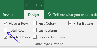
To enable the total row, go to the Table Tools Design tab and check the Total Row box found in the Table Style Options section.
You can temporarily disable the total row without losing the formulas you added to it. Excel will remember the formulas you had and they will appear when you enable it again.
Each cell in the total row has a drop down menu that allows you to pick various aggregating functions to summarize the column of data above.
You can also enter your own formulas. I’ve entered a SUMPRODUCT formula in the Unit Price total to sum the Quantity x Unit Price to calculate a total sale amount. Formulas don’t have to return a number, they can also be text results.
Constant numerical or text values are also allowed anywhere in the total row. In fact the leftmost column will usually contain the text Total by default.
Add a Total Row with a Right Click
You can also add the total row with a right click. Right click anywhere on the table and the choose Table and Total Row from the menu.
Add a Total Row with a Keyboard Shortcut
Another way to quickly add the total row is to place the active cell cursor inside your table and use the Ctrl + Shift + T keyboard shortcut.
Disable the Column Header Row
The column header row is enabled by default, but you can disable it. This doesn’t delete the column headers, it’s essentially like hiding them as you will still reference columns based on the column header name.
Go to the Table Tools Design tab and uncheck the Total Row box found in the Table Style Options section.
Add Bold Format to the First or Last Columns
You can enable a bold formatting on either your first or last column to highlight it and draw attention to them over other columns.
Go to the Table Tools Design tab and check either of the First Column or Last Column boxes (or both) found in the Table Style Options section.
Add Banded Rows or Columns
Banded rows are already enabled by default, but you can turn them off if you want. Banded columns are disabled by default, so you need to enable them if you want them.
To enable or disable either, go to the Table Tools Design tab and check or uncheck the Banded Rows or Banded Columns boxes found in the Table Style Options section.
I generally find banded rows are the most useful and if you enable banded columns at the same time, the table starts to look a little messy. I recommend one or the other and not both at the same time.
- Table with no banded rows or columns.
- Table with banded rows only.
- Table with banded columns only.
- Table with both banded rows and columns.
Table Filters
By default, the table filters option is enabled. You can disable them from the Table Tools Design tab by unchecking the Filter Button box found in the Table Style Options section.
You can also toggle the filters on or off from the active table by using the regular filter keyboard shortcut of Ctrl + Shift + L.
If you left click on any of the filters, it will bring up the familiar filter menu where you can sort your table and apply various filters depending on the type of data in the column.
The great thing about table filters is you can have them on multiple tables in the same sheet simultaneously. You will need to be careful though as filtered items in one table will affect the other tables if they share common rows. You can only have one set of filters at a time in a sheet of data without tables.
Total Row with Filters Applied
When you select a summary function from the drop down menu in the total row, Excel will create the corresponding SUBTOTAL formula. This SUBTOTAL formula ignores hidden and filtered items. So when you filter your table these summaries will update accordingly to exclude the filtered values.
Note that the SUMPRODUCT formula in the Unit Price column still includes all the filtered values while the SUBTOTAL sum formula in the Quantity column does not.
Column Headers Remain Visible When Scrolling
If you scroll down while the active cell is in a table, its column headers will remain visible along with the filter buttons. The table’s column headings will get promoted into the sheet’s column headings where we would normally see the alphabetic column name.
This is extremely handy when dealing with long tables as you won’t need to scroll back up to the top to see the column name or use the filters.
Automatically Include New Rows and Columns
If you type or copy and paste new data into the cells directly below a table, they will automatically be absorbed into the table.
The same thing happens when you type or copy and paste into the cells directly to the right of a table.
Automatically Fill Formulas Down the Entire Column
When you enter a formula inside a table it will automatically fill the formula down the entire column.
Even when a formula has already been entered and you add new data to the row directly below the table any existing formulas will automatically fill.
Editing an existing formula in any of the cells will also update the formula in the entire column. You’ll never forget to copy and paste down a formula again!
Turn Off the Auto Include and Auto Fill Settings
You can turn off the feature that automatically adds new rows or columns and fills down formulas.
Go to the File tab and select Options. Choose Proofing then press the AutoCorrect Options button. Navigate to the AutoFormat As You Type tab in the AutoCorrect dialog box.
Unchecking the Include new rows and columns in table option allows you to type directly underneath or to the right of a table without it absorbing the cells.
Unchecking the Fill formulas in tables to create calculated columns option means the formulas in a table will no longer automatically fill down the column.
Resize with the Handle
Every table comes with a Size Handle found in the bottom rightmost cell of the table.
When you hover the mouse over the handle, the cursor will turn into a double-sided diagonally slanting arrow and you can then click and drag to resize the table. You can either expand or contract the size. Data will be absorbed into the table or removed from it accordingly.
Resize with the Ribbon
You can also resize the table from the ribbon. Go to the Table Tools Design tab and press the Resize Table command in the Properties section.
The Resize Table dialog box will pop up and you’ll be able to select a new range for your table. Use the range selector icon to select a new range. You can select either a larger or smaller range, but The table headers will need to remain in the same row and the new table range must overlap the old table range.
Add a New Row with the Tab Key
You can add a new blank row to a table with the Tab key. Place the active cell cursor inside the table on the cell containing the sizing handle and press the Tab key.
The tab key act like a carriage return and the active cell is taken to the rightmost cell on a new line that’s added directly below.
This is a handy shortcut to know because when the total row is enabled, it’s not possible to add a new row by typing or copying and pasting data directly below the table.
Insert Rows or Columns
You can insert extra rows or columns into a table with a right click. Select a range in the table and right click then choose Insert from the menu. You can then either choose to insert Table Columns to the Left or Table Rows Above.
Table Columns to the Left will insert the number of columns selected to the left of the selection and the number of rows in the selection is ignored.
Table Rows Above will insert the number of rows selected just above the selection and the number of columns in the selection is ignored.
Delete Rows or Columns
Deleting rows or columns has a similar story to inserting them. Select a range in the table and right click then choose Delete from the menu. You can then either choose to delete Table Columns or Table Rows.
Formats in a Table Automatically Apply to New Rows
When you add new data to your table, you don’t need to worry about applying formatting to match the rest of the data above. Formatting will automatically fill down from above if the formatting has been applied to the entire column.
I’m not just talking about the table style formats. Other formatting like dates, numbers, fonts, alignments, borders, conditional formatting, cell colours etc. will all automatically fill down if they’ve been applied to the whole column.
If you’ve formatted all your numbers as a currency in a column and you add new data, it too will get the currency format applied to it.
You never need to worry about inconsistent formatting in your data.
Add a Slicer
You can add a slicer (or several) to a table for an easy to use filter and visual way to see what items the table is filtered on.
Go to the Table Tools Design tab and press the Insert Slicer button found in the Tools section.
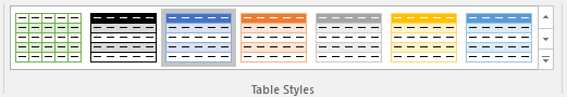
Change the Style
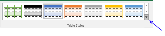
Changing the styling of a table is quick and easy. Go to the Table Tools Design select a new style from the selection found in the Table Styles section. If you left click the small downward arrow on the right hand side of the styles palette, it will expand to show all available options.
These table styles apply to the whole table and will also apply to any new rows or columns added later on.
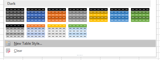
There are many options to choose from including light, medium and dark themes. As you hover over the various selections, you’ll be able to see a live preview in the worksheet. The style won’t actually change until you click on one though.
You can even create your own New Table Style.
Set a Default Table Style
You can set any of the styles available as the default so that when you create a new table you don’t need to change the style. Right click on the style you want to set as the default and then choose Set As Default from the menu.
Unfortunately, this is a workbook level setting and will only affect the current workbook. You will need to set the default for each workbook you create if you don’t want the application default option.
Only Print the Selected Table
When you place the active cell cursor inside a table and then try to print, there is an option to only print the selected table. Go to the Print menu screen by either going to the File tab and selecting Print or using the Ctrl + P keyboard shortcut, then select Print Selected Table in the settings.
This will remove any items from the print area that are not in the table.
Structured Referencing
Tables come with a useful feature called structured referencing which helps to make range references more readable. Ranges within a table can be referred to using a combination of the table name and column headings.
Instead of seeing a formula like this =SUM(D3:D9) you might see something like this =SUM(Sales[Quantity]) which is much easier to understand the meaning of.
This is why naming your table with a short descriptive name and column headings is important as it will improve the readability of the structured references!
When you reference specific parts of a table, Excel will create the reference for you so you don’t need to memorize the reference structure but it will help to understand it a bit.
Structured references can contain up to three parts.
- This is the table name. When referencing a range from inside the table this part of the reference is not required.
- These are range identifiers and identify certain parts of the reference for a table like the headers or total row.
- These are the column names and will either be a single column or a range of columns separated by a full colon.
Example of structured References for a Row
=Sales[@[Unit Price]]will reference a single cell in the body.=Sales[@[Product]:[Unit Price]]will reference part of the row from the Product column to the Unit Price column including all columns in between.=Sales[@]will reference the full row.
Example of Structured References for Columns
=Sales[Unit Price]will reference a single column and only include the body.=Sales[[#Headers],[#Data],[Unit Price]]will reference a single column and include the column header and body.=Sales[[#Data],[#Totals],[Unit Price]]will reference a single column and include the body and total row.=Sales[[#All],[Unit Price]]will reference a single column and include the column header, body and total row.
Example of Structured References for the Total Row
=Sales[#Totals]will reference the entire total row.=Sales[[#Totals],[Unit Price]]will reference a cell in the total row.=Sales[[#Totals],[Product]:[Unit Price]]will reference part of the total row from the Product column to the Unit Price column including all columns in between.
Example of Structured References for the Column Header Row
=Sales[#Headers]will reference the entire column header row.=Sales[[#Headers],[Order Date]]will reference a cell in the column header row.=Sales[[#Headers],[Product]:[Unit Price]]will reference part of the column header row from the Product column to the Unit Price column including all columns in between.
Example of Structured References for the Table Body
=Saleswill reference the entire body.=Sales[[#Headers],[#Data]]will reference the entire column header row and body.=Sales[[#Data],[#Totals]]will reference the entire body and total row.=Sales[#All]will reference the entire column header row, body and total row.
Using Intellisense
One of the great things about a table is the structured references will appear in Intellisense menus when writing formulas. This means you can easily write a formula using the structured references without remembering all the fields in your table.
After typing the first letter of the table name, the IntelliSense menu will show the table name among all the other objects starting with that letter. You can use the arrow keys to navigate to it and then press the Tab key to autocomplete the table name in your formula.
If you want to reference a part of the table, you can then type a [ to bring up all the available items in the table. Again, you can navigate with the arrow keys and then use the Tab key to autocomplete the field name. Then you can close the item with a ].
Turn Off Structured Referencing
If you’re not a fan of being forced to use the structured referencing system, then you can turn it off. Any formulas that have been entered using the structured referencing will remain and they will still work the same. You’ll also still be able to use structured references, Excel just won’t automatically create them for you.
To turn it off, go to the File tab and then select Options. Choose Formulas on the side pane and then uncheck the Use table names in formulas box and press the Ok button.
Summarize with a PivotTable
You can create a pivot table from your table in Table Tools Design tab, press the Summarize with PivotTable button found in the Tools section. This will bring up the Create PivotTable window and you can create a pivot table as usual.
This is the same as creating a pivot table from the Insert tab and doesn’t give any extra options specific to tables.
Remove Duplicates from a Table
You can create remove duplicate rows of data from your table in Table Tools Design tab, press the Remove Duplicates button found in the Tools section. This will bring up the Remove Duplicates window and delete duplicate values for one or more columns in the table.
This is the same as removing duplicates from the Data tab and doesn’t give any extra options specific to tables.
About the Author
John is a Microsoft MVP and qualified actuary with over 15 years of experience. He has worked in a variety of industries, including insurance, ad tech, and most recently Power Platform consulting. He is a keen problem solver and has a passion for using technology to make businesses more efficient.
Author: Oscar Cronquist Article last updated on February 07, 2023
An Excel Table is a very useful feature in Excel, it was introduced in Excel 2007. Earlier versions had this feature as well but it was then known as Excel Lists.
What can an Excel Table do for you? It will simplify your work with data, adding or removing data, filtering, totals, sorting, enhance readability using cell formatting, cell references, formulas, and more. I will go through all this in greater detail, keep on reading.
Table of Contents
- How to create an Excel Table
- How to name an Excel Table
- How to manipulate Excel Table data
- How to edit an Excel Table value
- How to delete an Excel Table value
- How to add a row
- How to add a column
- How to delete an Excel Table row
- How to delete an Excel Table column
- How to delete an Excel Table and keep values
- How to sort an Excel Table
- How to filter an Excel Table
- How to insert a total to an Excel Table and sum using a condition
- How do structured references work?
- Reference an entire Excel Table
- Reference Excel Table data
- Reference column headers
- Reference a column
- Reference a value on the same row
- How to use a formula in an Excel Table
- How to change Excel Table formatting
- How to show Excel Table totals
- List all tables in a workbook — Named ranges
- How to link a chart to an Excel Table
- How to link a drop-down list to an Excel Table (Data validation)
- Working with filtered Excel Tables
- How to quickly find an Excel Table in a workbook
- Count unique distinct values in a filtered Excel Table (Link)
- Extract unique distinct values from a filtered Excel Table (Link)
- Filter duplicate records [Excel Table] (Link)
1. How to create an Excel Table
Follow these simple steps to convert a cell range to a table:
- Go to tab «Insert» on the ribbon
- Select your data set
- Press with left mouse button on the «Table» button on tab «Insert»
- Press with left mouse button on the «OK» button if your table has headers, if not deselect the check box and press with left mouse button on «OK». Excel will automatically create headers for you.
- You have built an excel table
Tip! Use short cut keys CTRL + T to quickly build a table.
Back to top
2. How to name an Excel Table
I recommend you give the table and table headers descriptive names, for example, it will be easier to identify cell references to Excel Tables in formulas. Cell references are called structured references and you can read about these in this article as well.
- Select a cell in your table
- Excel automatically navigates to tab «Design» on your ribbon
- Change table name
- Press Enter
Back to top
3. How to manipulate Excel Table data
3.1 How to edit an Excel Table value
- Doublepress with left mouse button on any cell with left mouse button to start editing an Excel Table value.
- Use arrow keys to move the prompt between characters.
- Press Enter to apply changes or press CTRL + SHIFT + Enter to create an array formula.
3.2 How to delete an Excel Table value
- Press with left mouse button on with the left mouse button on any cell in the Excel Table to select it.
- Press Delete on the keyboard to remove the cell value.
3.3 How to add a row
- Press with left mouse button on with the left mouse button on any cell in the Excel Table to select it.
- Press the Tab key repeatedly until a new row is created.
A new row is created if you press the tab key with the lower right cell in the Excel Table selected. See the animated picture above.
Here is another way to create a new row.
- Select any cell right below the Excel Table the cell must be adjacent to the Excel Table for this to work.
- Type a value or a formula.
- Press Enter.
The Excel Table grows automatically when you add values adjacent to the Excel Table.
3.4 How to add a column
- Press with mouse on any cell adjacent to the Excel Table with the left mouse button to select it.
- Type a value or formula.
- Press Enter or CTRL + SHIFT + Enter.
The table expands automatically when you add values to adjacent cells, see the animated image above.
Add data to a cell adjacent to the table and the table expands automatically.
3.5 How to delete an Excel Table row
- Press with right mouse button on on one of the cells on the row you want to delete in the Excel Table.
- A popup menu appears, press with left mouse button on «Delete» on the popup menu.
- Another popup menu shows up, press with left mouse button on Table Rows.
This deletes the entire Excel Table row, it does not delete other values outside the Excel Table. At least not in Excel 365.
3.6 How to delete an Excel Table column
- Press with right mouse button on on any cell in an Excel Table. A popup menu appears.
- Press with mouse on «Delete» on the popup menu. Another popup menu shows up.
- Press with mouse on «Table Columns» .
3.7 How to delete an Excel Table and keep values

- Press with mouse on any cell in the Excel Table to select it. A tab named «Table Design» appears on the ribbon, this tab is not visible if not a cell in the Excel Table is sleected.
- Press with mouse on tab «Table Design» on the ribbon.
- Press with mouse on the «Convert to Range» button, see the image above.

The image above shows the Excel Table after converting to a normal range of cells. However, the cell formatting is still preserved.
Here is how to remove the cell formatting as well:
- Select the entire data set.
- Go to tab «Home» on the ribbon.
- Press with mouse on «Clear» button. A popup menu appears.
- Press with left mouse button on «Clear Formats».

Back to top
4. How to sort an Excel Table
Sorting a table is easy, press with left mouse button on any black triangle located at each header, a menu appears allowing you to quickly sort data in a descending or ascending order.
An arrow next to the black triangle indicates sort order. Sort Z to A (descending) shows you an arrow pointing down.
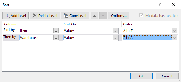
You can also sort on multiple columns, follow these steps.
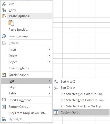
- Press with right mouse button on on a cell
- Press with left mouse button on Sort and then press with left mouse button on «Custom Sort…»

- Select column name to sort on and sort order then add more columns.

- Press with left mouse button on OK button to apply sort settings to table
The following article demonstartes how to sort a values in an excel defined table using a macro:
Recommended articles
Back to top
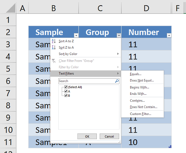
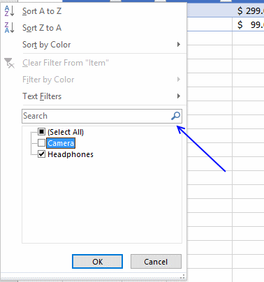
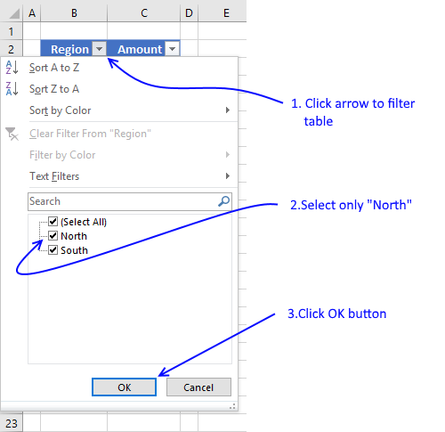
5. How to filter an Excel Table
- Press with mouse on a black triangle next to any header
- Select values you want to filter
- Press with left mouse button on OK button
See animated picture below.
Excel allows you to apply filters to multiple columns easily, repeat above steps with another column.
Use the search field to quickly find the value you want to filter, see picture below.
Back to top
6. How to insert a total to an Excel Table and sum using a condition
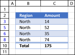
You can quickly sum values using table filtering.
Select a cell in the table, then go to tab «Design» on the ribbon.
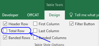
Press with left mouse button on «Checkbox» to enable «Total Row».
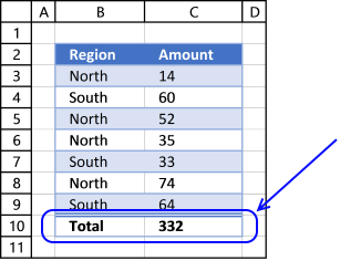
A row with totals appears on your table (332), see picture above.
Now filter the table, see instructions on picture below.
See how the total changes from 332 to 175.
Back to top
7. How do structured references work?
You are probably used to cell references like this one:
=SUM(E3:E6)
Creating a cell reference to a table column returns this instead, see picture below.
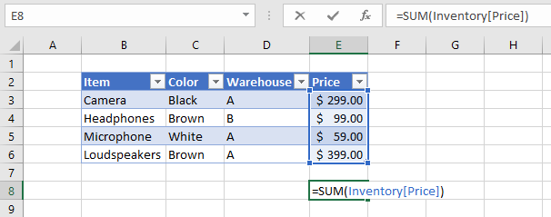
First the table name (Inventory) and then the column name enclosed with brackets [Price].
What is the purpose of structured references? The amazing thing with structured references is that if you add or remove values to a table the structured reference stays the same, no need to update cell references. In other words, they are dynamic.
7.1 Reference an entire Excel Table

The following structured reference returns the entire Excel Table including the column header names.
Formula in cell B9:
=Table1[#All]
Back to top
7.2 Reference Excel Table data

The following structured reference returns all Excel Table data, however, no the column header names.
Formula in cell B9:
=Table1
Back to top
7.3 Reference all column headers

The following structured reference returns all Excel Table column header names.
Formula in cell B9:
=Table1[#Headers]
Back to top
7.4 Reference a column

The following structured reference returns all Excel Table data from a given column.
Formula in cell B9:
=Table1[East]
Back to top

The following structured reference returns all Excel Table data from a given column including the column header name.
Formula in cell B9:
=Table1[[#All],[East]]
Back to top
7.5 Reference a value on the same row

The following structured reference returns an Excel Table value from a given column but on the same row as the formula is entered on.
Formula in cell G4:
=Table1[@North]
Back to top
8. How to use a formula in an Excel Table
The following example demonstrates what happens if I type a formula in an excel table. I want to multiply cell E3 with F3 in cell G3, see animated picture below.
Excel creates these structured cell references in cell G3 if I type = (equal sig) and then press with left mouse button on cell E3, type * (asterisk) and then press with left mouse button on cell F3:
=[@[‘#]]*[@Price]
@ (at) means cell value on same row as formula.
Excel also calculates the remaining cells in column G automatically, see animated picture above.
Creating a reference to the entire excel table and headers returns this: =Inventory[#All]
A reference to data in table looks like this: =Inventory
A reference to a table column returns: =Inventory[Warehouse]
A reference to a column header only looks like this: =Inventory[[#Headers],[Warehouse]]
Back to top
9. How to change Excel Table formatting
- Select a cell in excel table
- Go to tab «Design» on the ribbon

- Hover over a table style and see your table change

- If you like it press with left mouse button on it to select it
- Press with left mouse button on the black triangle to se even more table styles

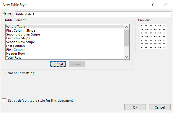
You can also build your own table style.
- Select a table cell
- Go to tab «Design»
- Press with left mouse button on black triangle
- Press with left mouse button on «New Table Style…»

- Enter a name for your table style

- Select a table element you want to change
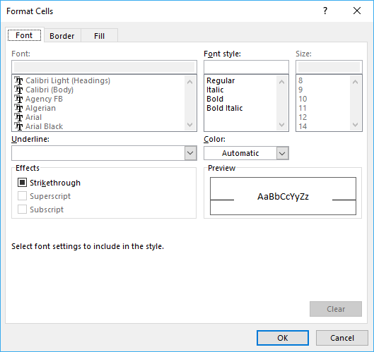
- Press with left mouse button on «Format» button

- Format as you like
- Press with left mouse button on OK button twice
Back to top
10. How to show Excel Table totals
- Press with mouse on a cell in an excel table
- Go to tab «Design»

- Press with left mouse button on «Total Row» check box

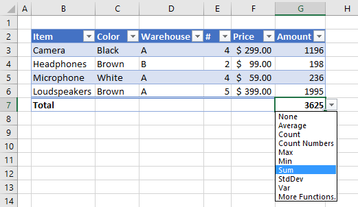
- Press with left mouse button on cell G7 and then on black triangle

- You can change how value in cell G7 is calculated, the menu has these formulas: Average, Count, Count Numbers, Max, Min, Sum, StdDev, Var and More Functions.
- If you press with left mouse button on «More Functions» a dialog box opens with formulas to choose from.

Back to top
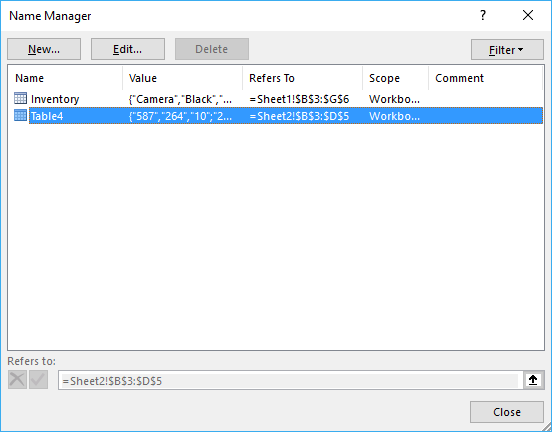
11. List all tables in workbook — Named ranges
The Name Manager contains a list of all named ranges and Excel tables in your workbook.
- Press with left mouse button on the «Formula» tab on the ribbon.
- Press with left mouse button on «Name Manager» button.

There are only Excel Tables in this workbook so the dialog box shows the Excel Table names, there are no named ranges in this workbook. See the image above.
Back to top
12. How to link a chart to an Excel Table
Combine chart and table to make use of dynamic cell references while filtering data.
More details here: How to create a dynamic chart
Back to top
13. How to link a drop-down list to an Excel Table (Data validation)
The following animation shows you a data validation list linked to a table.
Read this post if you are interested in the details:
How to use a table name in data validation lists and conditional formatting formulas
Back to top
14. Working with a filtered Excel Table
If you try to use a filtered table as a data source in a formula you are in for trouble, see animated picture below.
As you can see above the SUM function sums all values in table regardless of filtered or not.
I have written a few articles about this:
- Highlight duplicates in a filtered excel defined table
- Count unique distinct values in a filtered table
- Highlight unique values in a filtered excel table
- Populate a list box with visible unique values from an excel table (vba)
- Highlight unique values in a filtered excel table
- Extract unique distinct values from a filtered table (udf and array formula)
- Vlookup visible data in a table and return multiple values
Back to top
15. How to quickly find an Excel Table in a workbook
Excel lets you quickly focus on a table if you type the table name in the name box.
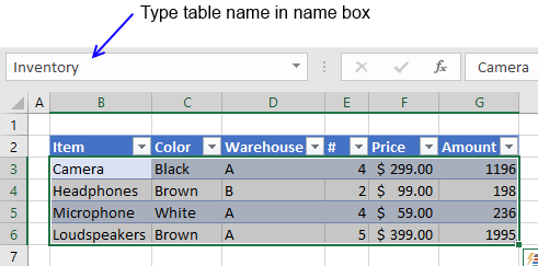
Back to top
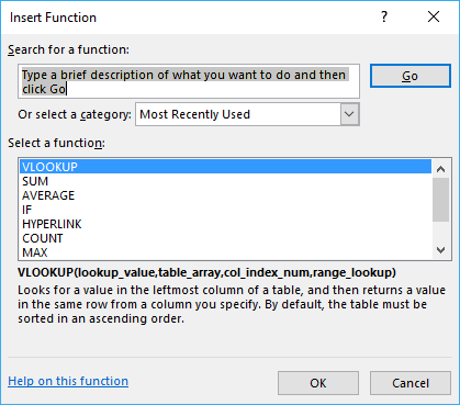
When you create an Excel table, Excel assigns a name to the table, and to each column header in the table. When you add formulas to an Excel table, those names can appear automatically as you enter the formula and select the cell references in the table instead of manually entering them. Here’s an example of what Excel does:
|
Instead of using explicit cell references |
Excel uses table and column names |
|---|---|
|
=Sum(C2:C7) |
=SUM(DeptSales[Sales Amount]) |
That combination of table and column names is called a structured reference. The names in structured references adjust whenever you add or remove data from the table.
Structured references also appear when you create a formula outside of an Excel table that references table data. The references can make it easier to locate tables in a large workbook.
To include structured references in your formula, click the table cells you want to reference instead of typing their cell reference in the formula. Let’s use the following example data to enter a formula that automatically uses structured references to calculate the amount of a sales commission.
|
Sales |
Region |
Sales |
% Commission |
Commission Amount |
|---|---|---|---|---|
|
Joe |
North |
260 |
10% |
|
|
Robert |
South |
660 |
15% |
|
|
Michelle |
East |
940 |
15% |
|
|
Erich |
West |
410 |
12% |
|
|
Dafna |
North |
800 |
15% |
|
|
Rob |
South |
900 |
15% |
-
Copy the sample data in the table above, including the column headings, and paste it into cell A1 of a new Excel worksheet.
-
To create the table, select any cell within the data range, and press Ctrl+T.
-
Make sure the My table has headers box is checked, and click OK.
-
In cell E2, type an equal sign (=), and click cell C2.
In the formula bar, the structured reference [@[Sales Amount]] appears after the equal sign.
-
Type an asterisk (*) directly after the closing bracket, and click cell D2.
In the formula bar, the structured reference [@[% Commission]] appears after the asterisk.
-
Press Enter.
Excel automatically creates a calculated column and copies the formula down the entire column for you, adjusting it for each row.
What happens when I use explicit cell references?
If you enter explicit cell references in a calculated column, it can be harder to see what the formula is calculating.
-
In your sample worksheet, click cell E2
-
In the formula bar, enter =C2*D2 and press Enter.
Notice that while Excel copies your formula down the column, it doesn’t use structured references. If, for example, you add a column between the existing columns C and D, you’d have to revise your formula.
How do I change a table name?
When you create an Excel table, Excel creates a default table name (Table1, Table2, and so on), but you can change the table name to make it more meaningful.
-
Select any cell in the table to show the Table Tools > Design tab on the ribbon.
-
Type the name you want in the Table Name box, and press Enter.
In our example data, we used the name DeptSales.
Use the following rules for table names:
-
Use valid characters Always start a name with a letter, an underscore character (_), or a backslash (). Use letters, numbers, periods, and underscore characters for the rest of the name. You can’t use «C», «c», «R», or «r» for the name, because they’re already designated as a shortcut for selecting the column or row for the active cell when you enter them in the Name or Go To box.
-
Don’t use cell references Names can’t be the same as a cell reference, such as Z$100 or R1C1.
-
Don’t use a space to separate words Spaces can’t be used in the name. You can use the underscore character (_) and period (.) as word separators. For example, DeptSales, Sales_Tax or First.Quarter.
-
Use no more than 255 characters A table name can have up to 255 characters.
-
Use unique table names Duplicate names aren’t allowed. Excel doesn’t distinguish between upper and lowercase characters in names so if you enter “Sales” but already have another name called “SALES» in the same workbook, you’ll be prompted to choose a unique name.
-
Use an object identifier If you plan on having a mix of tables, PivotTables and charts, it’s a good idea to prefix your names with the object type. For example: tbl_Sales for a sales table, pt_Sales for a sales PivotTable, and chrt_Sales for a sales chart, or ptchrt_Sales for a sales PivotChart. This keeps all of your names in an ordered list in the Name Manager.
Structured reference syntax rules
You can also enter or change structured references manually in the formula but to do that, it will help to understand structured reference syntax. Let’s go over the following formula example:
=SUM(DeptSales[[#Totals],[Sales Amount]],DeptSales[[#Data],[Commission Amount]])
This formula has the following structured reference components:
-
Table name:
DeptSales is a custom table name. It references the table data, without any header or total rows. You can use a default table name, such as Table1, or change it to use a custom name. -
Column specifier:
[Sales Amount]
and
[Commission Amount] are column specifiers that use the names of the columns they represent. They reference the column data, without any column header or total row. Always enclose specifiers in brackets as shown. -
Item specifier:
[#Totals] and [#Data] are special item specifiers that refer to specific portions of the table, such as the total row. -
Table specifier:
[[#Totals],[Sales Amount]] and [[#Data],[Commission Amount]] are table specifiers that represent the outer portions of the structured reference. Outer references follow the table name, and you enclose them in square brackets. -
Structured reference:
(DeptSales[[#Totals],[Sales Amount]] and DeptSales[[#Data],[Commission Amount]] are structured references, represented by a string that begins with the table name and ends with the column specifier.
To create or edit structured references manually, use these syntax rules:
-
Use brackets around specifiers All table, column, and special item specifiers need to be enclosed in matching brackets ([ ]). A specifier that contains other specifiers requires outer matching brackets to enclose the inner matching brackets of the other specifiers. For example: =DeptSales[[Sales Person]:[Region]]
-
All column headers are text strings But they don’t require quotes when they’re used in a structured reference. Numbers or dates, such as 2014 or 1/1/2014, are also considered text strings. You can’t use expressions with column headers. For example, the expression DeptSalesFYSummary[[2014]:[2012]] won’t work.
Use brackets around column headers with special characters If there are special characters, the entire column header needs to be enclosed in brackets, which means that double brackets are required in a column specifier. For example: =DeptSalesFYSummary[[Total $ Amount]]
Here’s the list of special characters that need extra brackets in the formula:
-
Tab
-
Line feed
-
Carriage return
-
Comma (,)
-
Colon (:)
-
Period (.)
-
Left bracket ([)
-
Right bracket (])
-
Pound sign (#)
-
Single quotation mark (‘)
-
Double quotation mark («)
-
Left brace ({)
-
Right brace (})
-
Dollar sign ($)
-
Caret (^)
-
Ampersand (&)
-
Asterisk (*)
-
Plus sign (+)
-
Equal sign (=)
-
Minus sign (-)
-
Greater than symbol (>)
-
Less than symbol (<)
-
Division sign (/)
-
At sign (@)
-
Backslash ()
-
Exclamation point (!)
-
Left parenthesis (()
-
Right parenthesis ())
-
Percent sign (%)
-
Question mark (?)
-
Backtick (`)
-
Semicolon (;)
-
Tilde (~)
-
Underscore (_)
-
Use an escape character for some special characters in column headers Some characters have special meaning and require the use of a single quotation mark (‘) as an escape character. For example: =DeptSalesFYSummary[‘#OfItems]
Here’s the list of special characters that need an escape character (‘) in the formula:
-
Left bracket ([)
-
Right bracket (])
-
Pound sign(#)
-
Single quotation mark (‘)
-
At sign (@)
Use the space character to improve readability in a structured reference You can use space characters to improve the readability of a structured reference. For example: =DeptSales[ [Sales Person]:[Region] ] or =DeptSales[[#Headers], [#Data], [% Commission]]
It’s recommended to use one space:
-
After the first left bracket ([)
-
Preceding the last right bracket (]).
-
After a comma.
Reference operators
For more flexibility in specifying ranges of cells, you can use the following reference operators to combine column specifiers.
|
This structured reference: |
Refers to: |
By using the: |
Which is cell range: |
|---|---|---|---|
|
=DeptSales[[Sales Person]:[Region]] |
All of the cells in two or more adjacent columns |
: (colon) range operator |
A2:B7 |
|
=DeptSales[Sales Amount],DeptSales[Commission Amount] |
A combination of two or more columns |
, (comma) union operator |
C2:C7, E2:E7 |
|
=DeptSales[[Sales Person]:[Sales Amount]] DeptSales[[Region]:[% Commission]] |
The intersection of two or more columns |
(space) intersection operator |
B2:C7 |
Special item specifiers
To refer to specific portions of a table, such as just the totals row, you can use any of the following special item specifiers in your structured references.
|
This special item specifier: |
Refers to: |
|---|---|
|
#All |
The entire table, including column headers, data, and totals (if any). |
|
#Data |
Just the data rows. |
|
#Headers |
Just the header row. |
|
#Totals |
Just the total row. If none exists, then it returns null. |
|
#This Row or @ or @[Column Name] |
Just the cells in the same row as the formula. These specifiers can’t be combined with any other special item specifiers. Use them to force implicit intersection behavior for the reference or to override implicit intersection behavior and refer to single values from a column. Excel automatically changes #This Row specifiers to the shorter @ specifier in tables that have more than one row of data. But if your table has only one row, Excel doesn’t replace the #This Row specifier, which may cause unexpected calculation results when you add more rows. To avoid calculation problems, make sure you enter multiple rows in your table before you enter any structured reference formulas. |
Qualifying structured references in calculated columns
When you create a calculated column, you often use a structured reference to create the formula. This structured reference can be unqualified or fully qualified. For example, to create the calculated column, called Commission Amount, that calculates the amount of commission in dollars, you can use the following formulas:
|
Type of structured reference |
Example |
Comment |
|---|---|---|
|
Unqualified |
=[Sales Amount]*[% Commission] |
Multiplies the corresponding values from the current row. |
|
Fully qualified |
=DeptSales[Sales Amount]*DeptSales[% Commission] |
Multiples the corresponding values for each row for both columns. |
The general rule to follow is this: If you’re using structured references within a table, such as when you create a calculated column, you can use an unqualified structured reference, but if you use the structured reference outside of the table, you need to use a fully qualified structured reference.
Examples of using structured references
Here are some ways to use structured references.
|
This structured reference: |
Refers to: |
Which is cell range: |
|---|---|---|
|
=DeptSales[[#All],[Sales Amount]] |
All the cells in the Sales Amount column. |
C1:C8 |
|
=DeptSales[[#Headers],[% Commission]] |
The header of the % Commission column. |
D1 |
|
=DeptSales[[#Totals],[Region]] |
The total of the Region column. If there is no Totals row, then it returns null. |
B8 |
|
=DeptSales[[#All],[Sales Amount]:[% Commission]] |
All the cells in Sales Amount and % Commission. |
C1:D8 |
|
=DeptSales[[#Data],[% Commission]:[Commission Amount]] |
Just the data of the % Commission and Commission Amount columns. |
D2:E7 |
|
=DeptSales[[#Headers],[Region]:[Commission Amount]] |
Just the headers of the columns between Region and Commission Amount. |
B1:E1 |
|
=DeptSales[[#Totals],[Sales Amount]:[Commission Amount]] |
The totals of the Sales Amount through Commission Amount columns. If there is no Totals row, then it returns null. |
C8:E8 |
|
=DeptSales[[#Headers],[#Data],[% Commission]] |
Just the header and the data of % Commission. |
D1:D7 |
|
=DeptSales[[#This Row], [Commission Amount]] or =DeptSales[@Commission Amount] |
The cell at the intersection of the current row and the Commission Amount column. If used in the same row as a header or total row, this will return a #VALUE! error. If you type the longer form of this structured reference (#This Row) in a table with multiple rows of data, Excel automatically replaces it with the shorter form (@). They both work the same. |
E5 (if the current row is 5) |
Strategies for working with structured references
Consider the following when you work with structured references.
-
Use Formula AutoComplete You may find that using Formula AutoComplete is very useful when you enter structured references and to ensure the use of correct syntax. For more information, see Use Formula AutoComplete.
-
Decide whether to generate structured references for tables in semi-selections By default, when you create a formula, clicking a cell range within a table semi-selects the cells and automatically enters a structured reference instead of the cell range in the formula. This semi-selection behavior makes it much easier to enter a structured reference. You can turn this behavior on or off by selecting or clearing the Use table names in formulas check box in the File > Options > Formulas > Working with formulas dialog.
-
Use workbooks with external links to Excel tables in other workbooks If a workbook contains an external link to an Excel table in another workbook, that linked source workbook must be open in Excel to avoid #REF! errors in the destination workbook that contains the links. If you open the destination workbook first and #REF! errors appear, they will be resolved if you then open the source workbook. If you open the source workbook first, you should see no error codes.
-
Convert a range to a table and a table to a range When you convert a table to a range, all cell references change to their equivalent absolute A1 style references. When you convert a range to a table, Excel doesn’t automatically change any cell references of this range to their equivalent structured references.
-
Turn off column headers You can toggle table column headers on and off from the table Design tab > Header Row. If you turn off table column headers, structured references that use column names aren’t affected, and you can still use them in formulas. Structured references that refer directly to the table headers (e.g. =DeptSales[[#Headers],[%Commission]]) will result in #REF.
-
Add or delete columns and rows to the table Because table data ranges often change, cell references for structured references adjust automatically. For example, if you use a table name in a formula to count all the data cells in a table, and you then add a row of data, the cell reference automatically adjusts.
-
Rename a table or column If you rename a column or table, Excel automatically changes the use of that table and column header in all structured references that are used in the workbook.
-
Move, copy, and fill structured references All structured references remain the same when you copy or move a formula that uses a structured reference.
Note: Copying a structured reference and doing a fill of a structured reference are not the same thing. When you copy, all the structured references remain the same, while when you fill a formula, fully qualified structured references adjust the column specifiers like a series as summarized in the following table.
|
If the fill direction is: |
And while filling, you |
Then: |
|---|---|---|
|
Up or down |
Nothing |
There is no column specifier adjustment. |
|
Up or down |
Ctrl |
Column specifiers adjust like a series. |
|
Right or left |
None |
Column specifiers adjust like a series. |
|
Up, down, right, or left |
Shift |
Instead of overwriting values in current cells, current cell values are moved and column specifiers are inserted. |
Need more help?
You can always ask an expert in the Excel Tech Community or get support in the Answers community.
Related Topics
Overview of Excel tables
Video: Create and format an Excel table
Total the data in an Excel table
Format an Excel table
Resize a table by adding or removing rows and columns
Filter data in a range or table
Convert a table to a range
Excel table compatibility issues
Export an Excel table to SharePoint
Overviews of formulas in Excel
Bottom line: Learn why using an Excel Table as the source of a pivot table can save time and prevent errors.
Skill level: Beginner
Do You Love Excel Tables?
Excel Tables are one of those hidden gems of Excel. They are an extremely useful feature that can save us a lot of time when working with lists or sets of data.
Tables are becoming more popular, but a lot of people still don’t use them. I believe this is mainly due to the “weird” formulas that are used in Tables.
The formulas are called structured references, and they can be turned off if you don’t want to use them. Structured reference formulas are actually very useful once you understand how they work, but that is a whole other topic.
Checkout my video on a Beginner’s Guide to Excel Tables if you are not using this feature yet.
In this post I want to focus on why you should use Tables for the source data range of your pivot tables. So let’s get into it.
#1 – Adding New Data & Preventing Embarrassment
Have you ever added new data to the bottom of your source data, and then forgot to update the pivot table(s) to include the new rows of data?
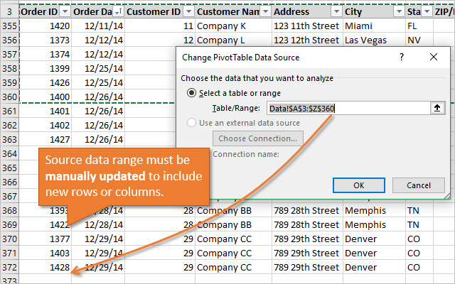
The better question is, how many times has this happened to you? I’ll admit that this has happened more than once in my career, and it’s an embarrassing mistake.
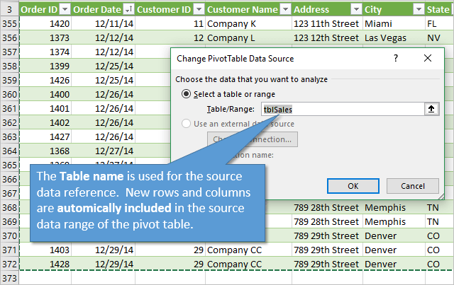
Using Excel Table as the source data range of the pivot table prevents this mistake. When we paste data below a Table, the Table automatically extends to include the new data. Since the pivot table(s) reference the Table name as source data range, instead of a range reference, the new data is automatically included in the pivot table.
The only step you have to remember is to refresh the pivot table(s).
For me, this one reason alone is enough to always use Tables as the source data range.
#2 – Eliminate Maintenance on Multiple Pivot Tables
Typically we create multiple pivot table reports on one source data range. If we use a regular range for the source, we have to update every single pivot table when we add new data (rows or columns) to the source. This can be very time consuming if your workbook has dozens of pivot tables. There is always a chance we miss one, and again suffer from that embarrassing mistake…
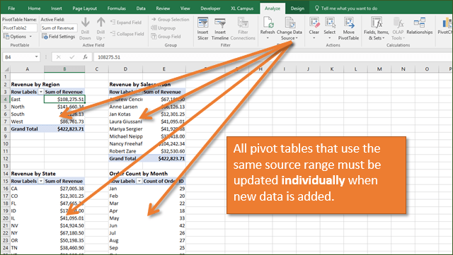
When we use a Table as the source range, we do NOT need to change the source data range when we add new rows or columns to the end of the table.
All pivot tables that use the Table as the source data range will be refreshed because they share the same pivot cache. This means you can just refresh one pivot table, and all the others that use the same Table as the source will also be updated. Here is an article that explains more about the pivot cache and how pivot tables are connected.
#3 – Prevent Errors When Creating Pivot Tables
Pivot tables are picky, and require the source data to be in the right format and layout. I have a source data checklist that explains more about the 8 steps to formatting your source data.
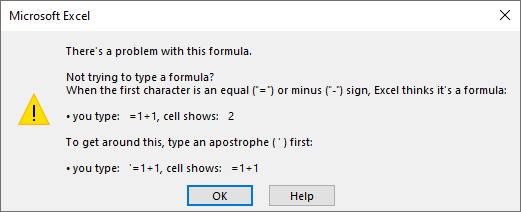
One of those steps is deleting blank columns. We cannot create a pivot table from a source data range that contains blank columns. Excel gives us the following error message.
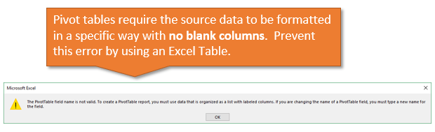
The PivotTable field name is not valid. To create a PivotTable report, you must use data that is organized in a list with labeled columns. If you are changing the name of a PivotTable field, you must type a new name for the field.
This error message causes a lot of confusion. It should say, “Your data cannot contain blank columns or a header row that contains blank cells. Each column must have a descriptive name in the first (header) row of the source data range.”
The advantage of using an Excel Table is that it does NOT allow us to have blank cells in the header (top) row. All cells in the header row must contain a value. If they don’t, a value will be inserted in the cell. The value will be “Column” with a number after it: Column1, Column2, etc.
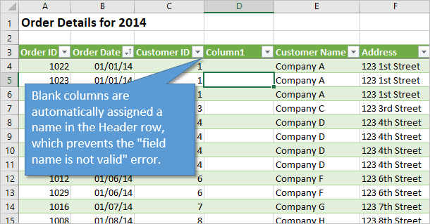
Even if your source data has blank columns, those columns will get a header name when you insert the Table. This means you will not get that error message when creating a pivot table.
#4 – Avoid Whole Column References
Another “trick” I see used a lot to avoid maintenance is to use whole column references for the source data range. We can just reference the entire columns of the source data range in the pivot table, so we don’t have to change the last row number when new data is added.
In theory this would help eliminate the issues I explained in #1 and #2 above. However, whole column references come with their own set of potential issues.
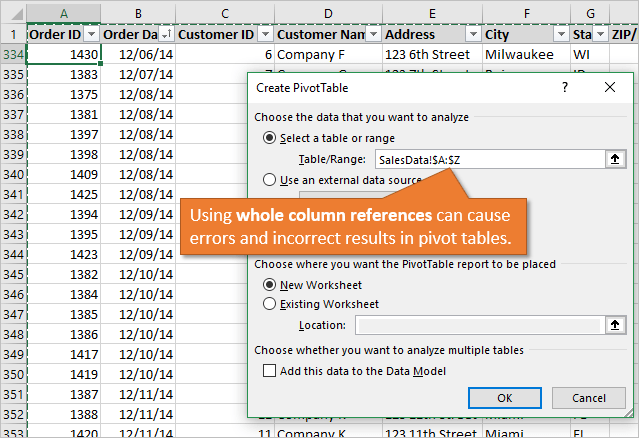
Here’s a quick list of reasons to not use whole column references:
- If any data is accidentally added to the bottom of the sheet below the actual data range, it will also be included in the pivot table. This can lead to bloated pivot tables, incorrect results, and issues with the grouping feature not working due to blank cells in a column.
- You cannot add formulas below the actual data range to help tie out numbers.
- Whole column references do not include new columns added to the right of the data range. This still requires maintenance to update the source ranges.
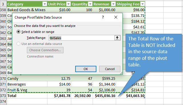
If we use an Excel Table instead we don’t have to worry about these issues. We can add formulas below the data range, and we can also use the Totals Row feature of the Table to summarize columns. The Totals Row is NOT included in the pivot table.
#5 – Prevent the Filter Controls Error with Connected Slicers
If you’ve seen my video series on pivot tables and dashboards, then you know we can connect a slicer to multiple pivot tables and pivot charts to create interactive dashboards. This is a very powerful feature of Excel.
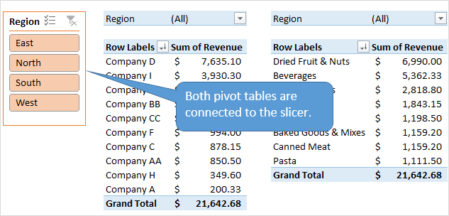
However, if we use a regular range as the source of our pivot tables, we first have to disconnect the slicers before changing the source data range. We then have to reconnect all the slicers after the update. This can be very time consuming, and is a tedious manual process.
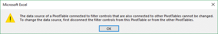
I have an article on how pivot tables and slicers are connected, that explains this issue in more detail. The ultimate solution is to use a Table as the source range. This prevents the error and we do not have to disconnect the slicers to add new data to the source.
How to Use Tables with Pivot Tables
Now that we know why to use Tables, you might be wondering how to set it up.
Creating a New Pivot Table from a Table
Here are instructions to create a new pivot table from a Table:
- Select any cell in the Table.
- Go to the Insert Tab on the Ribbon and click the “Pivot Table” button. There is also a “Summarize with Pivot Table” button on the Table Design tab that does the same thing.
- The Create PivotTable window will open and the Table name should automatically be referenced in the Table/Range box.
- Choose where you want the pivot table to be placed, new or existing worksheet.
- Click OK.
The new pivot table will be created using the Table as the source data range.
Changing the Data Source for an Existing Pivot Table
If you have an existing pivot table that uses a regular range as the source, you can change it to use a Table as the source. Here’s an animated screencast with the instructions below:
- Go to the source data range and Insert a Table (Insert tab on the Ribbon > Table).
- Go to the existing pivot table and select a cell inside the pivot table.
- Go to the Options/Analyze tab on the Ribbon and click the “Change Data Source” button.
- The Change PivotTable Source Data window will open.
- Select a cell inside the Table.
- Press Ctrl+A. This shortcut will select all cells in the Table and automatically insert the Table Name in the Table/Range box.
- Click OK.
The pivot table will now use the Table as the source data range, and benefit from all the reasons mentioned in this article.
Other Reasons To Use Tables with Pivot Tables?
Well, there are 5 good reasons to start using Tables with Pivot Tables. Checkout my video on a beginner’s guide to Tables for more reasons to use this awesome feature of Excel.
Tables are also used with tools like Power Query and Power Pivot, so it’s good to get experience with how Tables work.
Do you have any other reasons to use Tables with pivot tables. Please leave a comment below with suggestions or questions. Thank you! 🙂
Free Training Webinar on Pivot Tables
Next week I’m hosting a free webinar on “The 5 Secrets to Understanding Pivot Tables”.
During the free webinar I am going to explain how we can use pivot tables to quickly summarize our data for interactive reports and dashboards.
I am going to share my screen and jump into Excel to explain how pivot tables work, and some of the most critical steps for using this powerful tool. This is one of those Excel skills that will help you save time with your job, and impress the boss. 🙂

Click here to register for the webinar
Spots are limited so get registered today. It’s free!
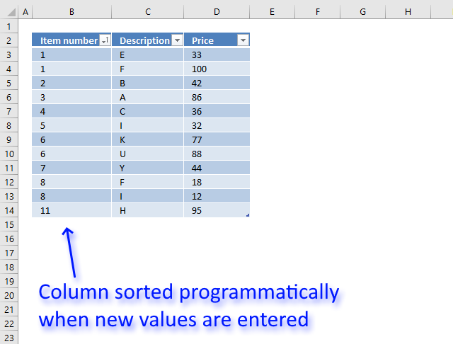
Excel Tables expand automatically whenever new data is added to the bottom. This feature alone makes Tables one of the most powerful tools within the Excel users toolkit. A Table can be used as the source data for a chart and within a named range, both of which benefit from the auto-expand feature. Data validation lists would also benefit from the auto-expand feature… but it just doesn’t work; an oversight on Microsoft’s part (in my opinion).
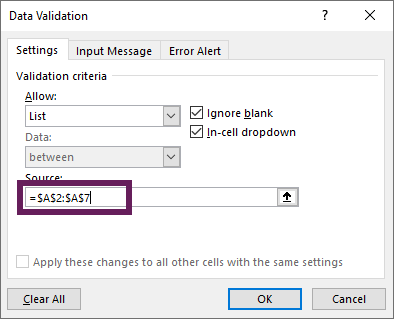
The following data validation settings look like it should work. It should use the column called Animals from a Table called myList.
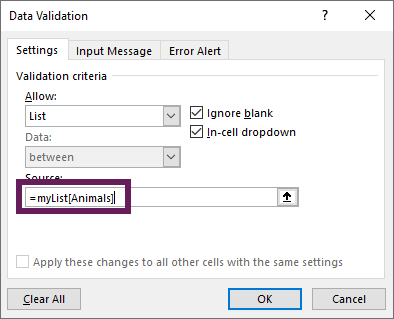
But Excel will show an error message instead.
What can you use to solve this problem? I’ve got three solutions for you:
- Normal cell references over a Table
- Named range of the Table column
- INDIRECT function
Let’s look at each of these and you can decide which is the best option for your situation.
Download the example file: Click the link below to download the example file used for this post:
Watch the video
Watch the video on YouTube.
Example Data
The examples in this post use the following data:
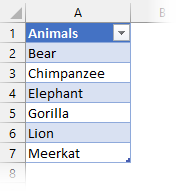
The Table name is myList (I know, it’s not a great name, but it will work for the examples).
Normal cell references over a Table
If we use standard cell references, the data validation list will be static. Each time a new item is added to the list either the data validation source will need to be updated, or the new items will need to be added within the existing list range. However, if we create the data validation list using normal cell references over a Table column, it will expand.
Look at the screenshot below. The cells $A$2:$A$7 are the same cells as the reference myList[Animals] would be for a Table.
It looks like it would behave like a standard static list. But somehow Excel knows, and the data validation list expands when values are added to the Table. Try it for yourself.
Problems with this approach
There are some big problems with this approach:
- If the data validation list is on a separate sheet to the Table, it will not expand.
- This method only works if the cells selected include the entire Table column (i.e., in our example, if you reference $A$4:$A$7 it will not expand when a new item is added as it is not the whole Table column).
Due to the issues noted above, it is probably best to avoid this method.
Named range of the Table column
Named ranges will accept a Table column as the source, and a data validation list will accept a Named range. Therefore, we can take a two-step approach to achieve the same result.
Create the named range
To create the named range, click Formulas -> Define Name
The New Name window will open. Give the named range a name (myDVList in the example below) and set the Refers to box to the name of the Table and column.
Finally, Click OK. The named range has now been created.
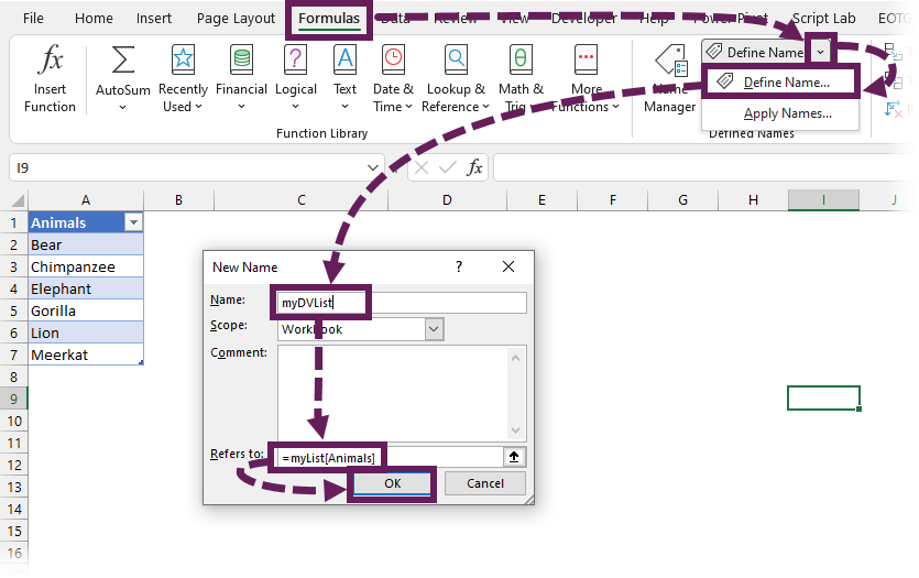
The formula used in the screenshot above is.
=myList[Animals]
If the list only has one column, it is possible to refer to just the Table without the column name (just like the screenshot below.
=myList
Add the named range to the data validation list
The screenshot below shows the named range added to the data validation list box.

The data validation list will now expand whenever new items are added to the Table.
Key points about this method
In relation to this method, there are a few things to be aware of:
- This is a two-stage process, which takes a little longer to set-up.
- If the Table or Column names change the named range automatically updates to reflect the changes.
While it takes longer to set-up, this method is the one that is least likely to break.
INDIRECT Function
The INDIRECT function will convert text into a Range which Excel will recognize and use in calculations. For example, if Cell A2 contains the text “A1” you can write =INDIRECT(A2) and Excel will convert that to the cell reference =A1.
We can use the INDIRECT function with the Table and column reference as text and Excel will understand this.
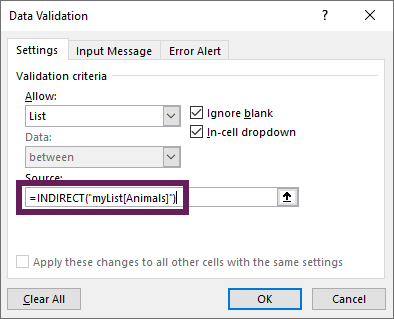
The formula used in the screenshot above is.
=INDIRECT("myList[Animals]")
If the list only has one column, it is possible to refer to just the Table.
=INDIRECT("myList")
The data validation list will now expand whenever new items are added to the Table.
Warning about this method
There is one key thing to be aware of; the Table and column names are now hardcoded into the INDIRECT formula. If either of these change the data validation list will cease to work as the formula cannot find the source data.
Which method to choose?
So, with three options to choose from, the question is which is the best. Personally, I prefer the named range option. I use named ranges often, so it fits with my way of working. However, if I have to create a lot of named ranges, I may be lazy and choose the INDIRECT method. I don’t advise using the standard cell references over a table as it won’t work across worksheets.

About the author
Hey, I’m Mark, and I run Excel Off The Grid.
My parents tell me that at the age of 7 I declared I was going to become a qualified accountant. I was either psychic or had no imagination, as that is exactly what happened. However, it wasn’t until I was 35 that my journey really began.
In 2015, I started a new job, for which I was regularly working after 10pm. As a result, I rarely saw my children during the week. So, I started searching for the secrets to automating Excel. I discovered that by building a small number of simple tools, I could combine them together in different ways to automate nearly all my regular tasks. This meant I could work less hours (and I got pay raises!). Today, I teach these techniques to other professionals in our training program so they too can spend less time at work (and more time with their children and doing the things they love).
Do you need help adapting this post to your needs?
I’m guessing the examples in this post don’t exactly match your situation. We all use Excel differently, so it’s impossible to write a post that will meet everybody’s needs. By taking the time to understand the techniques and principles in this post (and elsewhere on this site), you should be able to adapt it to your needs.
But, if you’re still struggling you should:
- Read other blogs, or watch YouTube videos on the same topic. You will benefit much more by discovering your own solutions.
- Ask the ‘Excel Ninja’ in your office. It’s amazing what things other people know.
- Ask a question in a forum like Mr Excel, or the Microsoft Answers Community. Remember, the people on these forums are generally giving their time for free. So take care to craft your question, make sure it’s clear and concise. List all the things you’ve tried, and provide screenshots, code segments and example workbooks.
- Use Excel Rescue, who are my consultancy partner. They help by providing solutions to smaller Excel problems.
What next?
Don’t go yet, there is plenty more to learn on Excel Off The Grid. Check out the latest posts: