This cell excel vba - Word и Excel - помощь в работе с программами

Содержание

Excel VBA Ranges and Cells
Ranges and Cells in VBA
Cell Address
A1 Notation
R1C1 Notation
Range of Cells
A1 Notation
R1C1 Notation
Writing to Cells
Reading from Cells
Non Contiguous Cells
VBA Coding Made Easy
Intersection of Cells
Offset from a Cell or Range
Offset Syntax
Offset from a cell
Offset from a Range
Setting Reference to a Range
Resize a Range
Resize Syntax
OFFSET vs Resize
All Cells in Sheet
UsedRange
CurrentRegion
Range Properties
Last Cell in Sheet
Last Used Row Number in a Column
Last Used Column Number in a Row
Cell Properties
Common Properties
Cell Font
Copy and Paste
Paste All
Paste Special
AutoFit Contents
More Range Examples
For Each
Range Address
Range to Array
Array to Range
Sum Range
Count Range
VBA Code Examples Add-in
Get, Set, or Change Cell value in Excel VBA
Set Cell Value
Set the value to a single cell
Get Cell Value
Change Cell Values

Excel VBA Ranges and Cells

In this Article

Ranges and Cells in VBA

Excel spreadsheets store data in Cells. Cells are arranged into Rows and Columns. Each cell can be identified by the intersection point of it’s row and column (Exs. B3 or R3C2).

An Excel Range refers to one or more cells (ex. A3:B4)

Cell Address

A1 Notation

In A1 notation, a cell is referred to by it’s column letter (from A to XFD) followed by it’s row number(from 1 to 1,048,576). This is called a cell address.

In VBA you can refer to any cell using the Range Object.

R1C1 Notation

In R1C1 Notation a cell is referred by R followed by Row Number then letter ‘C’ followed by the Column Number. eg B4 in R1C1 notation will be referred by R4C2. In VBA you use the Cells Object to use R1C1 notation:

Range of Cells

A1 Notation

To refer to a more than one cell use a “:” between the starting cell address and last cell address. The following will refer to all the cells from A1 to D10:

R1C1 Notation

To refer to a more than one cell use a “,” between the starting cell address and last cell address. The following will refer to all the cells from A1 to D10:

Writing to Cells

To write values to a cell or contiguous group of cells, simple refer to the range, put an = sign and then write the value to be stored:

Reading from Cells

To read values from cells, simple refer to the variable to store the values, put an = sign and then refer to the range to be read:

Note: To store values from a range of cells, you need to use an Array instead of a simple variable.

Non Contiguous Cells

To refer to non contiguous cells use a comma between the cell addresses:

VBA Coding Made Easy

Stop searching for VBA code online. Learn more about AutoMacro — A VBA Code Builder that allows beginners to code procedures from scratch with minimal coding knowledge and with many time-saving features for all users!

Intersection of Cells

To refer to non contiguous cells use a space between the cell addresses:

Offset from a Cell or Range

Using the Offset function, you can move the reference from a given Range (cell or group of cells) by the specified number_of_rows, and number_of_columns.

Offset Syntax

Offset from a cell

Offset from a Range

Setting Reference to a Range

To assign a range to a range variable: declare a variable of type Range then use the Set command to set it to a range. Please note that you must use the SET command as RANGE is an object:

Resize a Range

Resize method of Range object changes the dimension of the reference range:

Top-left cell of the Resized range is same as the top-left cell of the original range

Resize Syntax

OFFSET vs Resize

Offset does not change the dimensions of the range but moves it by the specified number of rows and columns. Resize does not change the position of the original range but changes the dimensions to the specified number of rows and columns.

All Cells in Sheet

The Cells object refers to all the cells in the sheet (1048576 rows and 16384 columns).

UsedRange

UsedRange property gives you the rectangular range from the top-left cell used cell to the right-bottom used cell of the active sheet.

CurrentRegion

CurrentRegion property gives you the contiguous rectangular range from the top-left cell to the right-bottom used cell containing the referenced cell/range.

Range Properties

You can get Address, row/column number of a cell, and number of rows/columns in a range as given below:

Last Cell in Sheet

You can use Rows.Count and Columns.Count properties with Cells object to get the last cell on the sheet:

Last Used Row Number in a Column

END property takes you the last cell in the range, and End(xlUp) takes you up to the first used cell from that cell.

Last Used Column Number in a Row

END property takes you the last cell in the range, and End(xlToLeft) takes you left to the first used cell from that cell.

You can also use xlDown and xlToRight properties to navigate to the first bottom or right used cells of the current cell.

Cell Properties

Common Properties

Here is code to display commonly used Cell Properties

Cell Font

Cell.Font object contains properties of the Cell Font:

Copy and Paste

Paste All

Ranges/Cells can be copied and pasted from one location to another. The following code copies all the properties of source range to destination range (equivalent to CTRL-C and CTRL-V)

Paste Special

Selected properties of the source range can be copied to the destination by using PASTESPECIAL option:

Here are the possible options for the Paste option:

AutoFit Contents

Size of rows and columns can be changed to fit the contents using AutoFit:

More Range Examples

It is recommended that you use Macro Recorder while performing the required action through the GUI. It will help you understand the various options available and how to use them.

For Each

It is easy to loop through a range using For Each construct as show below:

At each iteration of the loop one cell in the range is assigned to the variable cell and statements in the For loop are executed for that cell. Loop exits when all the cells are processed.

Sort is a method of Range object. You can sort a range by specifying options for sorting to Range.Sort. The code below will sort the columns A:C based on key in cell C2. Sort Order can be xlAscending or xlDescending. Header:= xlYes should be used if first row is the header row.

Find is also a method of Range Object. It find the first cell having content matching the search criteria and returns the cell as a Range object. It return Nothing if there is no match.

Use FindNext method (or FindPrevious) to find next(previous) occurrence.

Following code will change the font to “Arial Black” for all cells in the range which start with “John”:

Following code will replace all occurrences of “To Test” to “Passed” in the range specified:

It is important to note that you must specify a range to use FindNext. Also you must provide a stopping condition otherwise the loop will execute forever. Normally address of the first cell which is found is stored in a variable and loop is stopped when you reach that cell again. You must also check for the case when nothing is found to stop the loop.

Range Address

Use Range.Address to get the address in A1 Style

Use xlReferenceStyle (default is xlA1) to get addres in R1C1 style

This is useful when you deal with ranges stored in variables and want to process for certain addresses only.

Range to Array

It is faster and easier to transfer a range to an array and then process the values. You should declare the array as Variant to avoid calculating the size required to populate the range in the array. Array’s dimensions are set to match number of values in the range.

Array to Range

After processing you can write the Array back to a Range. To write the Array in the example above to a Range you must specify a Range whose size matches the number of elements in the Array.

Use the code below to write the Array to the range D1:D5:

Please note that you must Transpose the Array if you write it to a row.

Sum Range

You can use many functions available in Excel in your VBA code by specifying Application.WorkSheetFunction. before the Function Name as in the example above.

Count Range

Written by: Vinamra Chandra

VBA Code Examples Add-in

Easily access all of the code examples found on our site.

Simply navigate to the menu, click, and the code will be inserted directly into your module. .xlam add-in.

Источник

Get, Set, or Change Cell value in Excel VBA

We use VBA to automate our tasks in excel. The idea of using VBA is to connect the interface of excel with the programming. One of the very most connections between them is by changing the cell values. The change in cell value by programming shows the power of VBA. In this article, we will see how to set, get and change the cell value.

Set Cell Value

Assigning a cell with a value can be achieved by very two famous functions in VBA i.e. Range and Cells function.

Range Function in VBA

The range function helps access the cells in the worksheet. To set the cell value using the range function, we use the .Value.

Syntax: Range(cell_name).Value = value_to_be_assinged.

Set the value to a single cell

If you want to assign ’11’ to cell A1, then the following are the steps:

Step 1: Use the Range function, in the double quotes type the cell name. Use .Value object function. For example, Range(“A1”).Value = 11.

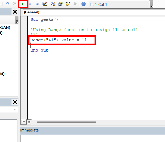
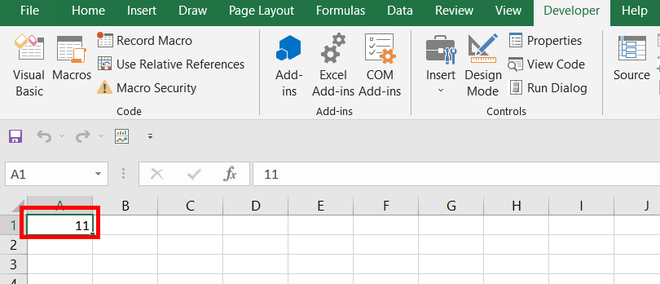
Step 2: Run your macro. The number 11 appears in cell A1.

Set the value to multiple cells at the same time

Remember the days, when your teacher gives you punishment, by making you write the homework 10 times, those were the hard days, but now the effort has exponentially reduced. You can set a value to a range of cells with just one line of code. If you want to write your name, for example, “Arushi” 10 times, in the range A2 to A11. Use range function. Following are the steps:

Step 1: Use the Range function, in the double quotes, write “Start_of_cell: End_of_cell”. Use .Value object function. For example, Range(“A2:A11”).Value = “Arushi”.

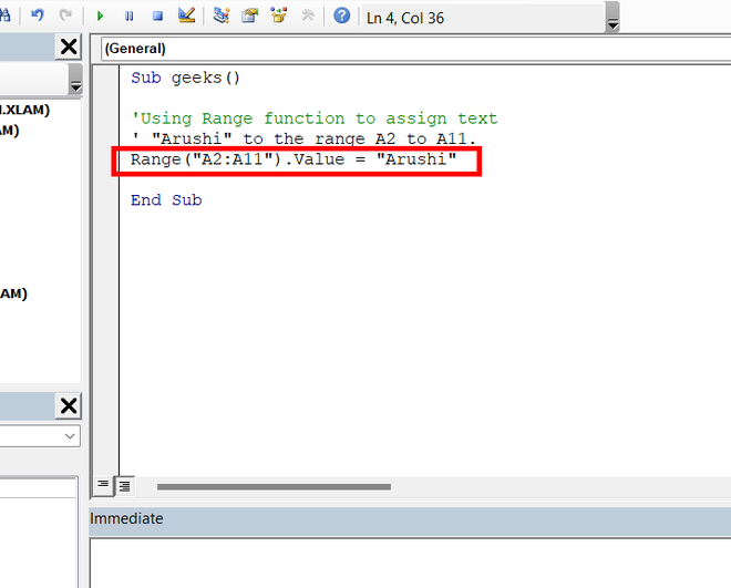
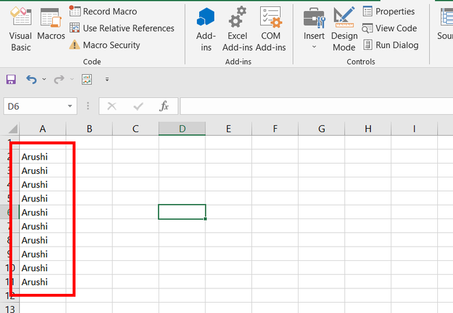
Step 2: Run your macro. The text “Arushi” appears from cell A2 to A11 inclusive.

Cells Function in VBA

The Cells function is similar to the range function and is also used to set the cell value in a worksheet by VBA. The difference lies in the fact that the Cells function can only set a single cell value at a time while the Range function can set multiple values at a time. Cells function use matrix coordinate system to access cell elements. For example, A1 can be written as (1, 1), B1 can be written as (1, 2), etc.

Syntax: Cells(row_number, column_number).Value = value_to_be_assign

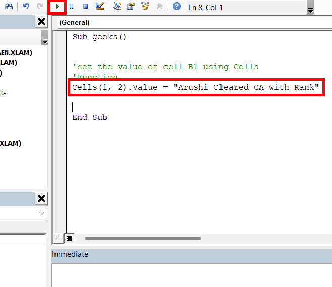
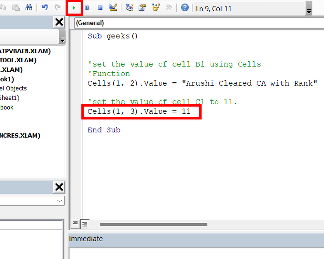
For example, you want to set the cell value to “Arushi cleared CA with Rank “, in cell B1. Also, set cell C1, to ‘1’. Following are the steps:

Step 1: Open your VBA editor. Use cells function, as we want to access cell B1, the matrix coordinates will be (1, 2). Type, Cells(1, 2).Value = “Arushi cleared CA with Rank” in the VBA code.

Step 2: To access cell C1, the matrix coordinates are (1, 3). Type, Cells(1, 3).Value = 1 in the VBA code.

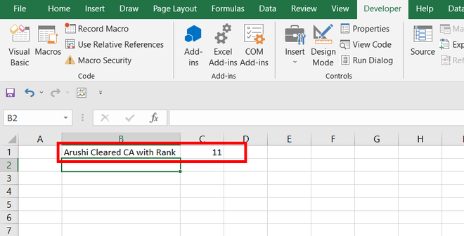
Step 3: Run your macro. The required text appears in cell B1, and a number appears in C1.

Setting Cell values by Active cell and the input box

There are other ways by which you can input your value in the cell in a worksheet.

Active Cell

You can set the cell value of a cell that is currently active. An active cell is the selected cell in which data is entered if you start typing. Use ActiveCell.Value object function to set the value either to text or to a number.

Syntax: ActiveCell.Value = value_to_be_assigned

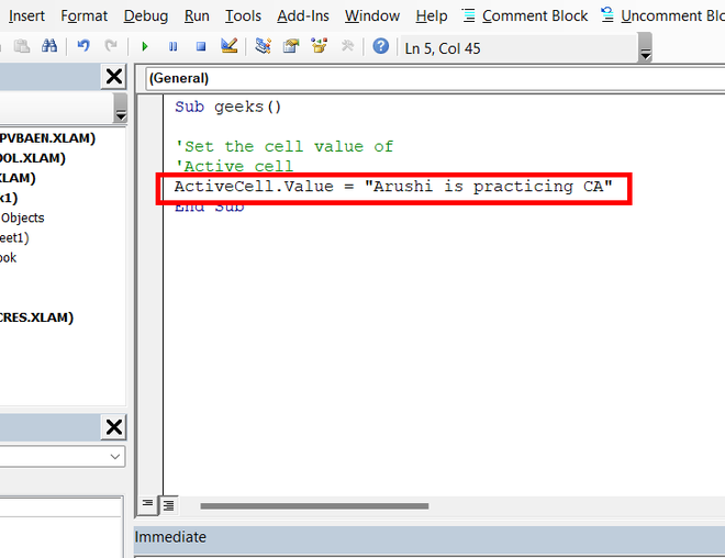
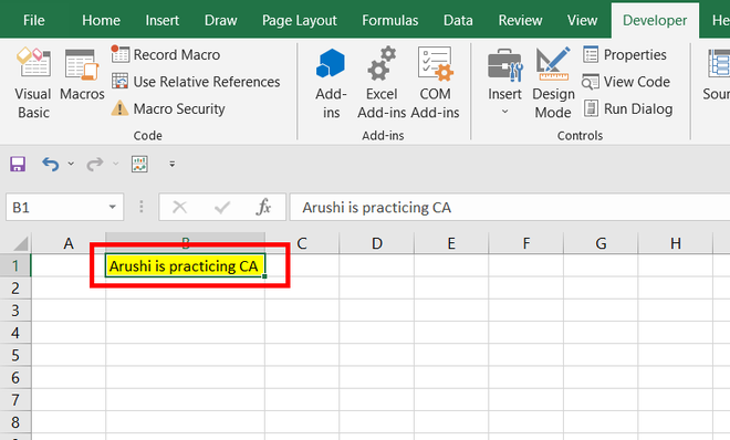
For example, you want to assign the active cell with a text i.e. “Arushi is practicing CA”, also want to change the color of the cell to yellow. Following are the steps:

Step 1: Use the ActiveCell object to access the currently selected cell in the worksheet. Use ActiveCell.Value function object to write the required text.

Step 2: Color the cell by using ActiveCell.Interior.Color function. For example, use vbYellow to set your cell color to yellow.

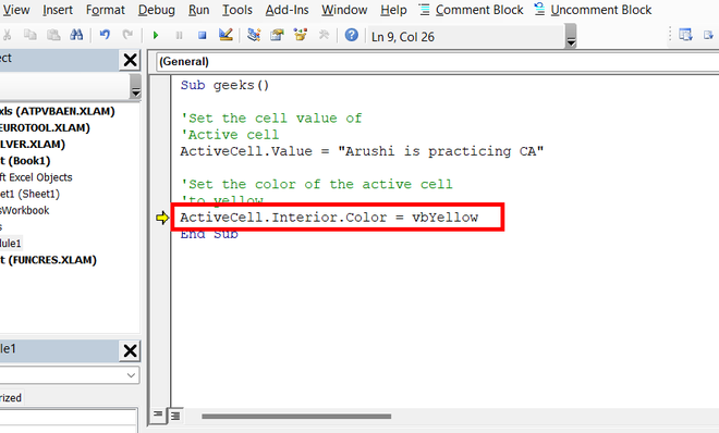
Step 3: Run your macro. The currently selected cell i.e. B1 has attained the requirements.

Input Box

You can use the input box to set the cell value in a worksheet. The input box takes the custom value and stores the result. This result could further be used to set the value of the cell. For example, set the cell value of A1, dynamically by taking input, from the input box.

Following are the steps

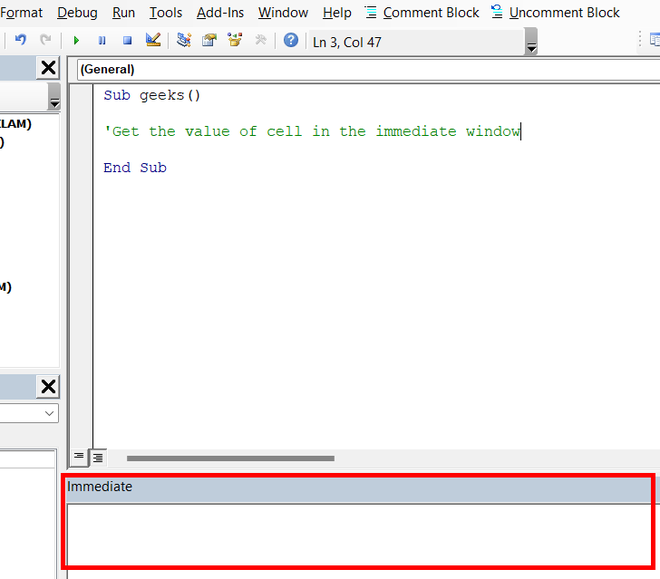
Step 1: Open your VBA editor. A sub-procedure name geeks() is created. Use the Range function to store the value given by the input box.

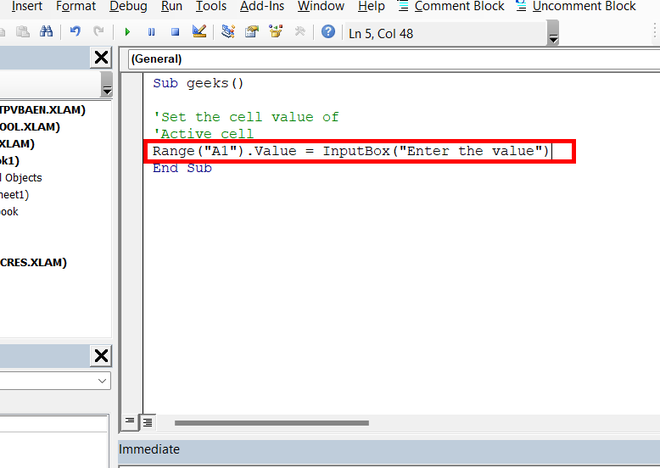
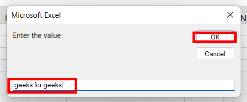
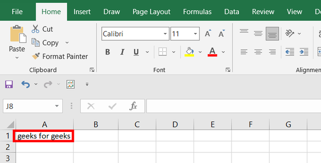
Step 2: Run your Macro. A dialogue-box name Microsoft Excel appears. Enter the value to be stored. For example, “geeks for geeks”. Click Ok.

Step 3: Open your worksheet. In cell A1, you will find the required text is written.

Get Cell Value

After setting the cell value, it’s very important to have a handsome knowledge of how to display the cell value. There can be two ways two get the cell value either print the value in the console or create a message box.

Print Cell Value in Console

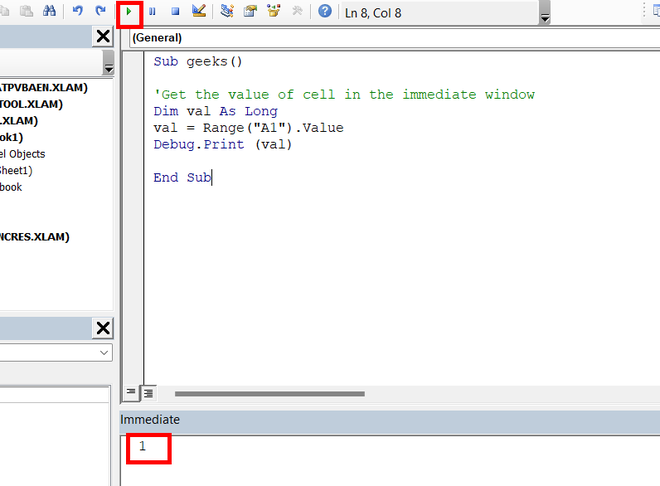
The console of the VBA editor is the immediate window. The immediate window prints the desired result in the VBA editor itself. The cell value can be stored in a variable and then printed in the immediate window. For example, you are given a cell A1 with the value ’11’, and you need to print this value in the immediate window.

Following are the steps

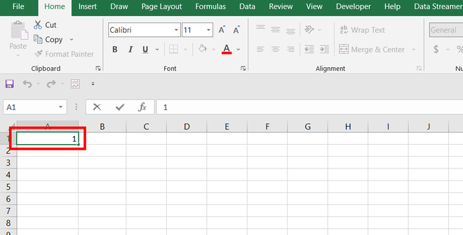
Step 1: Press Ctrl + G to open the immediate window.

Step 2: The cell value in A1 is 1.

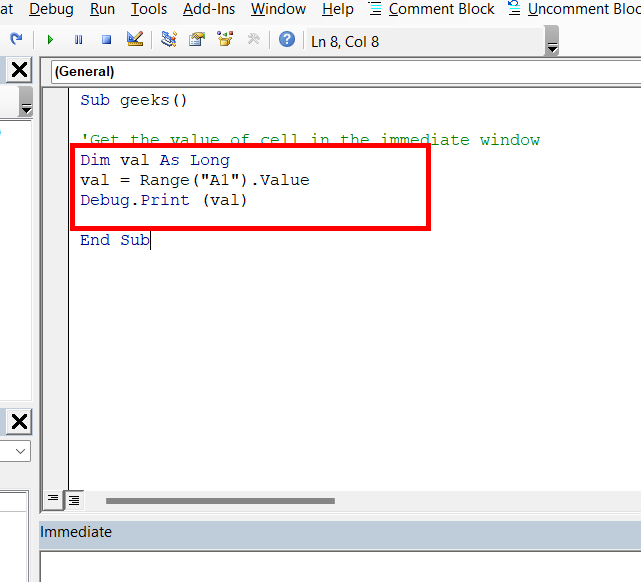
Step 3: Open your VBA editor. Declare a variable that could store the cell value. For example, Val is the variable that stores the cell value in A1. Use the Range function to access the cell value. After storing the cell value in the val, print the variable in the immediate window with the help of Debug.Print(val) function.

Step 4: Run your macro. The cell value in A1 is printed in the immediate window.

Print Cell Value in a Message Box

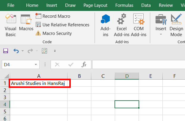
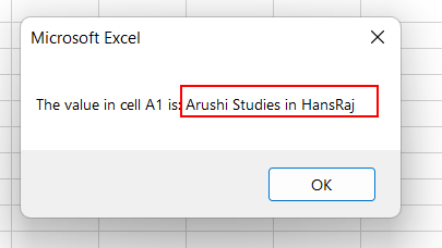
A message box can also be used to show the cell value in VBA. For example, a random string is given in cell A1 of your string i.e. “Arushi studies in Hansraj”. Now, if you want to display the cell value in A1, we can use Message Box to achieve this.

Following are the steps

Step 1: Open your VBA macro. Create a message box by using MsgBox. Use the Range(cell).Value function to access the cell value.

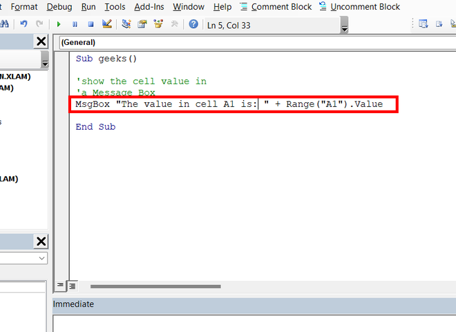
Step 2: Run your macro. A message box appears, which contains the cell value of A1.

Change Cell Values

The value, once assigned to the cell value, can be changed. Cell values are like variables whose values can be changed any number of times. Either you can simply reassign the cell value or you can use different comparators to change the cell value according to a condition.

By reassigning the Cell Value

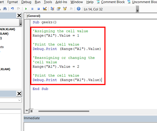
You can change the cell value by reassigning it. In the below example, the value of cell A1 is initially set to 1, but later it is reassigned to 2.

Following are the steps

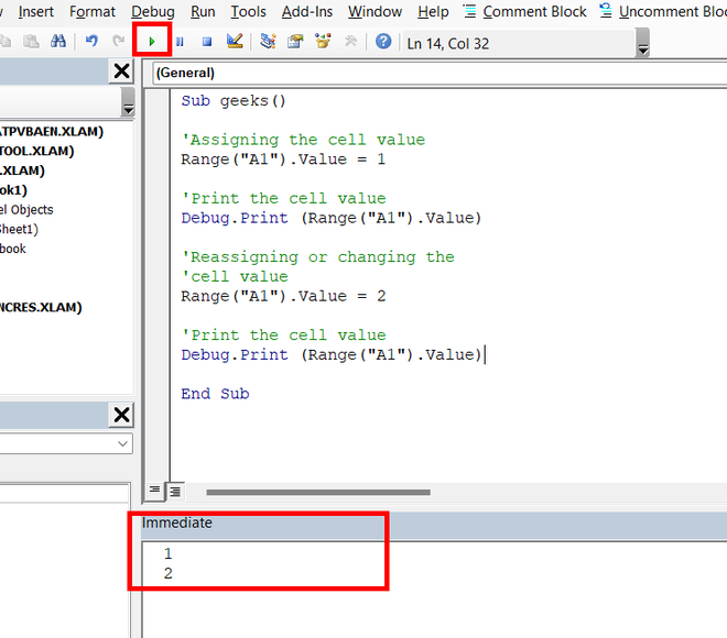
Step 1: Open your VBA code editor. Initially, the value of cell A1 is assigned to 1. This initial value is printed in the immediate window. After that, we changed the value of cell A1 to 2. Now, if we print the A1 value in the immediate window, it comes out to be 2.

Step 2: The immediate window shows the output as 1 and 2.

Changing cell value with some condition

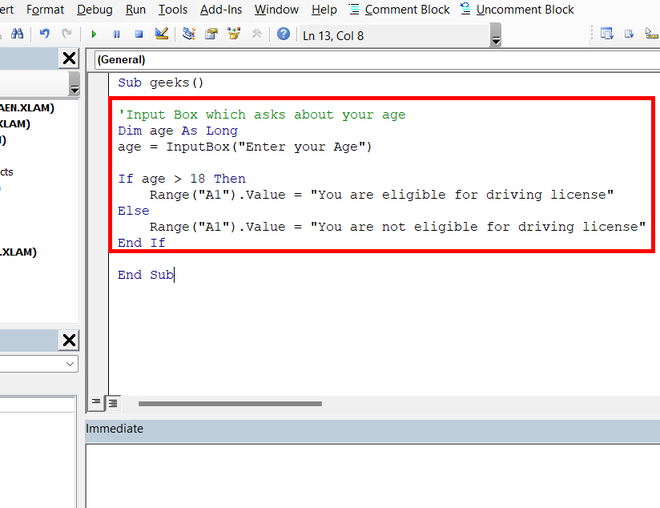
We can use if-else or switch-case statements to change the cell value with some condition. For example, if your age is greater than 18 then you can drive else you cannot drive. You can output your message according to this condition.

Following are the steps

Step 1: A code is written in the image below, which tells whether you are eligible for a driving license or not. If your age is greater than 18 then cell A1 will be assigned with the value, “You are eligible for the driving license”, else A1 will be assigned with “You are not eligible for driving license”.

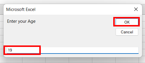
Step 2: Run your macro. An input box appears. Enter your age. For example, 19.

Step 3: According to the age added the cell value will be assigned.

Источник

Всё о работе с ячейками в Excel-VBA: обращение, перебор, удаление, вставка, скрытие, смена имени.

Содержание:

Table of Contents:

Что такое ячейка Excel?
Способы обращения к ячейкам
- Выбор и активация
- Получение и изменение значений ячеек
  - Ячейки открытой книги
  - Ячейки закрытой книги
- Перебор ячеек
- Перебор в произвольном диапазоне
Свойства и методы ячеек
- Имя ячейки
- Адрес ячейки
- Размеры ячейки
Запуск макроса активацией ячейки

2 нюанса:

Я почти везде стараюсь использовать ThisWorkbook (а не, например, ActiveWorkbook) для обращения к текущей книге, в которой написан этот код (считаю это наиболее безопасным для новичков способом обращения к книгам, чтобы случайно не внести изменения в другие книги). Для экспериментов можете вставлять этот код в модули, коды книги, либо листа, и он будет работать только в пределах этой книги.
Я использую английский эксель и у меня по стандарту листы называются Sheet1, Sheet2 и т.д. Если вы работаете в русском экселе, то замените Thisworkbook.Sheets(«Sheet1») на Thisworkbook.Sheets(«Лист1»). Если этого не сделать, то вы получите ошибку в связи с тем, что пытаетесь обратиться к несуществующему объекту. Можно также заменить на Thisworkbook.Sheets(1), но это менее безопасно.

Что такое ячейка Excel?

В большинстве мест пишут: «элемент, образованный пересечением столбца и строки». Это определение полезно для людей, которые не знакомы с понятием «таблица». Для того, чтобы понять чем на самом деле является ячейка Excel, необходимо заглянуть в объектную модель Excel. При этом определения объектов «ряд», «столбец» и «ячейка» будут отличаться в зависимости от того, как мы работаем с файлом.

Объекты в Excel-VBA. Пока мы работаем в Excel без углубления в VBA определение ячейки как «пересечения» строк и столбцов нам вполне хватает, но если мы решаем как-то автоматизировать процесс в VBA, то о нём лучше забыть и просто воспринимать лист как «мешок» ячеек, с каждой из которых VBA позволяет работать как минимум тремя способами:

по цифровым координатам (ряд, столбец),
по адресам формата А1, B2 и т.д. (сценарий целесообразности данного способа обращения в VBA мне сложно представить)
по уникальному имени (во втором и третьем вариантах мы будем иметь дело не совсем с ячейкой, а с объектом VBA range, который может состоять из одной или нескольких ячеек). Функции и методы объектов Cells и Range отличаются. Новичкам я бы порекомендовал работать с ячейками VBA только с помощью Cells и по их цифровым координатам и использовать Range только по необходимости.

Все три способа обращения описаны далее

Как это хранится на диске и как с этим работать вне Excel? С точки зрения хранения и обработки вне Excel и VBA. Сделать это можно, например, сменив расширение файла с .xls(x) на .zip и открыв этот архив.

Пример содержимого файла Excel:

Далее xl -> worksheets и мы видим файл листа

Содержимое файла:

То же, но более наглядно:

<?xml version="1.0" encoding="UTF-8" standalone="yes"?>
<worksheet xmlns="http://schemas.openxmlformats.org/spreadsheetml/2006/main" xmlns:r="http://schemas.openxmlformats.org/officeDocument/2006/relationships" xmlns:mc="http://schemas.openxmlformats.org/markup-compatibility/2006" mc:Ignorable="x14ac xr xr2 xr3" xmlns:x14ac="http://schemas.microsoft.com/office/spreadsheetml/2009/9/ac" xmlns:xr="http://schemas.microsoft.com/office/spreadsheetml/2014/revision" xmlns:xr2="http://schemas.microsoft.com/office/spreadsheetml/2015/revision2" xmlns:xr3="http://schemas.microsoft.com/office/spreadsheetml/2016/revision3" xr:uid="{00000000-0001-0000-0000-000000000000}">
	<dimension ref="B2:F6"/>
	<sheetViews>
		<sheetView tabSelected="1" workbookViewId="0">
			<selection activeCell="D12" sqref="D12"/>
		</sheetView>
	</sheetViews>
	<sheetFormatPr defaultRowHeight="14.4" x14ac:dyDescent="0.3"/>
	<sheetData>
		<row r="2" spans="2:6" x14ac:dyDescent="0.3">
			<c r="B2" t="s">
				<v>0</v>
			</c>
		</row>
		<row r="3" spans="2:6" x14ac:dyDescent="0.3">
			<c r="C3" t="s">
				<v>1</v>
			</c>
		</row>
		<row r="4" spans="2:6" x14ac:dyDescent="0.3">
			<c r="D4" t="s">
				<v>2</v>
			</c>
		</row>
		<row r="5" spans="2:6" x14ac:dyDescent="0.3">
			<c r="E5" t="s">
				<v>0</v></c>
		</row>
		<row r="6" spans="2:6" x14ac:dyDescent="0.3">
			<c r="F6" t="s"><v>3</v>
		</c></row>
	</sheetData>
	<pageMargins left="0.7" right="0.7" top="0.75" bottom="0.75" header="0.3" footer="0.3"/>
</worksheet>

Как мы видим, в структуре объектной модели нет никаких «пересечений». Строго говоря рабочая книга — это архив структурированных данных в формате XML. При этом в каждую «строку» входит «столбец», и в нём в свою очередь прописан номер значения данного столбца, по которому оно подтягивается из другого XML файла при открытии книги для экономии места за счёт отсутствия повторяющихся значений. Почему это важно. Если мы захотим написать какой-то обработчик таких файлов, который будет напрямую редактировать данные в этих XML, то ориентироваться надо на такую модель и структуру данных. И правильное определение будет примерно таким: ячейка — это объект внутри столбца, который в свою очередь находится внутри строки в файле xml, в котором хранятся данные о содержимом листа.

Способы обращения к ячейкам

Выбор и активация

Почти во всех случаях можно и стоит избегать использования методов Select и Activate. На это есть две причины:

Это лишь имитация действий пользователя, которая замедляет выполнение программы. Работать с объектами книги можно напрямую без использования методов Select и Activate.
Это усложняет код и может приводить к неожиданным последствиям. Каждый раз перед использованием Select необходимо помнить, какие ещё объекты были выбраны до этого и не забывать при необходимости снимать выбор. Либо, например, в случае использования метода Select в самом начале программы может быть выбрано два листа вместо одного потому что пользователь запустил программу, выбрав другой лист.

Можно выбирать и активировать книги, листы, ячейки, фигуры, диаграммы, срезы, таблицы и т.д.

Отменить выбор ячеек можно методом Unselect:

Selection.Unselect

Отличие выбора от активации — активировать можно только один объект из раннее выбранных. Выбрать можно несколько объектов.

Если вы записали и редактируете код макроса, то лучше всего заменить Select и Activate на конструкцию With … End With. Например, предположим, что мы записали вот такой макрос:

Sub Macro1()
' Macro1 Macro
    Range("F4:F10,H6:H10").Select 'выбрали два несмежных диапазона зажав ctrl
    Range("H6").Activate          'показывает только то, что я начал выбирать второй диапазон с этой ячейки (она осталась белой). Это действие ни на что не влияет
    With Selection.Interior       
        .Pattern = xlSolid
        .PatternColorIndex = xlAutomatic
        .Color = 65535            'залили желтым цветом, нажав на кнопку заливки на верхней панели
        .TintAndShade = 0
        .PatternTintAndShade = 0
    End With
End Sub

Почему макрос записался таким неэффективным образом? Потому что в каждый момент времени (в каждой строке) программа не знает, что вы будете делать дальше. Поэтому в записи выбор ячеек и действия с ними — это два отдельных действия. Этот код лучше всего оптимизировать (особенно если вы хотите скопировать его внутрь какого-нибудь цикла, который должен будет исполняться много раз и перебирать много объектов). Например, так:

Sub Macro11()
'
' Macro1 Macro
    Range("F4:F10,H6:H10").Select '1. смотрим, что за объект выбран (что идёт до .Select)
    Range("H6").Activate
    With Selection.Interior       '2. понимаем, что у выбранного объекта есть свойство interior, с которым далее идёт работа
        .Pattern = xlSolid
        .PatternColorIndex = xlAutomatic
        .Color = 65535
        .TintAndShade = 0
        .PatternTintAndShade = 0
    End With
End Sub



Sub Optimized_Macro()
    With Range("F4:F10,H6:H10").Interior '3. переносим объект напрямую в конструкцию With вместо Selection
' ////// Здесь я для надёжности прописал бы ещё Thisworkbook.Sheet("ИмяЛиста") перед Range,
' ////// чтобы минимизировать риск любых случайных изменений других листов и книг
' ////// With Thisworkbook.Sheet("ИмяЛиста").Range("F4:F10,H6:H10").Interior
        .Pattern = xlSolid               '4. полностью копируем всё, что было записано рекордером внутрь блока with
        .PatternColorIndex = xlAutomatic
        .Color = 55555                   '5. здесь я поменял цвет на зеленый, чтобы было видно, работает ли код при поочерёдном запуске двух макросов
        .TintAndShade = 0
        .PatternTintAndShade = 0
    End With
End Sub

Пример сценария, когда использование Select и Activate оправдано:

Допустим, мы хотим, чтобы во время исполнения программы мы одновременно изменяли несколько листов одним действием и пользователь видел какой-то определённый лист. Это можно сделать примерно так:

Sub Select_Activate_is_OK()
Thisworkbook.Worksheets(Array("Sheet1", "Sheet3")).Select 'Выбираем несколько листов по именам
Thisworkbook.Worksheets("Sheet3").Activate 'Показываем пользователю третий лист
'Далее все действия с выбранными ячейками через Select будут одновременно вносить изменения в оба выбранных листа

'Допустим, что тут мы решили покрасить те же два диапазона:
Range("F4:F10,H6:H10").Select
    Range("H6").Activate
    With Selection.Interior       
        .Pattern = xlSolid
        .PatternColorIndex = xlAutomatic
        .Color = 65535
        .TintAndShade = 0
        .PatternTintAndShade = 0
    End With

End Sub

Единственной причиной использовать этот код по моему мнению может быть желание зачем-то показать пользователю определённую страницу книги в какой-то момент исполнения программы. С точки зрения обработки объектов, опять же, эти действия лишние.

Получение и изменение значений ячеек

Значение ячеек можно получать/изменять с помощью свойства value.

'Если нужно прочитать / записать значение ячейки, то используется свойство Value
a = ThisWorkbook.Sheets("Sheet1").Cells (1,1).Value 'записать значение ячейки А1 листа "Sheet1" в переменную "a"
ThisWorkbook.Sheets("Sheet1").Cells (1,1).Value = 1  'задать значение ячейки А1 (первый ряд, первый столбец) листа "Sheet1"

'Если нужно прочитать текст как есть (с форматированием), то можно использовать свойство .text:
ThisWorkbook.Sheets("Sheet1").Cells (1,1).Text = "1" 
a = ThisWorkbook.Sheets("Sheet1").Cells (1,1).Text

'Когда проявится разница:
'Например, если мы считываем дату в формате "31 декабря 2021 г.", хранящуюся как дата
a = ThisWorkbook.Sheets("Sheet1").Cells (1,1).Value 'эапишет как "31.12.2021"
a = ThisWorkbook.Sheets("Sheet1").Cells (1,1).Text  'запишет как "31 декабря 2021 г."

Ячейки открытой книги

К ячейкам можно обращаться:

'В книге, в которой хранится макрос (на каком-то из листов, либо в отдельном модуле или форме)
ThisWorkbook.Sheets("Sheet1").Cells(1,1).Value        'По номерам строки и столбца
ThisWorkbook.Sheets("Sheet1").Cells(1,"A").Value      'По номерам строки и букве столбца
ThisWorkbook.Sheets("Sheet1").Range("A1").Value       'По адресу - вариант 1
ThisWorkbook.Sheets("Sheet1").[A1].Value              'По адресу - вариант 2
ThisWorkbook.Sheets("Sheet1").Range("CellName").Value 'По имени ячейки (для этого ей предварительно нужно его присвоить)

'Те же действия, но с использованием полного названия рабочей книги (книга должна быть открыта)
Workbooks("workbook.xlsm").Sheets("Sheet1").Cells(1,1).Value 'По номерам строки и столбца
Workbooks("workbook.xlsm").Sheets("Sheet1").Cells(1,"A").Value                'По номерам строки и букве столбца
Workbooks("workbook.xlsm").Sheets("Sheet1").Range("A1").Value                 'По адресу - вариант 1
Workbooks("workbook.xlsm").Sheets("Sheet1").[A1].Value                        'По адресу - вариант 2
Workbooks("workbook.xlsm").Sheets("Sheet1").Range("CellName").Value           'По имени ячейки (для этого ей предварительно нужно его присвоить)

Ячейки закрытой книги

Если нужно достать или изменить данные в другой закрытой книге, то необходимо прописать открытие и закрытие книги. Непосредственно работать с закрытой книгой не получится, потому что данные в ней хранятся отдельно от структуры и при открытии Excel каждый раз производит расстановку значений по соответствующим «слотам» в структуре. Подробнее о том, как хранятся данные в xlsx см выше.

Workbooks.Open Filename:="С:closed_workbook.xlsx"    'открыть книгу (она становится активной)
a = ActiveWorkbook.Sheets("Sheet1").Cells(1,1).Value  'достать значение ячейки 1,1
ActiveWorkbook.Close False                            'закрыть книгу (False => без сохранения)

Скачать пример, в котором можно посмотреть, как доставать и как записывать значения в закрытую книгу.

Код из файла:

Option Explicit
Sub get_value_from_closed_wb() 'достать значение из закрытой книги
Dim a, wb_path, wsh As String
wb_path = ThisWorkbook.Sheets("Sheet1").Cells(2, 3).Value 'get path to workbook from sheet1
wsh = ThisWorkbook.Sheets("Sheet1").Cells(3, 3).Value
Workbooks.Open Filename:=wb_path
a = ActiveWorkbook.Sheets(wsh).Cells(3, 3).Value
ActiveWorkbook.Close False
ThisWorkbook.Sheets("Sheet1").Cells(4, 3).Value = a
End Sub

Sub record_value_to_closed_wb() 'записать значение в закрытую книгу
Dim wb_path, b, wsh As String
wsh = ThisWorkbook.Sheets("Sheet1").Cells(3, 3).Value
wb_path = ThisWorkbook.Sheets("Sheet1").Cells(2, 3).Value 'get path to workbook from sheet1
b = ThisWorkbook.Sheets("Sheet1").Cells(5, 3).Value 'get value to record in the target workbook
Workbooks.Open Filename:=wb_path
ActiveWorkbook.Sheets(wsh).Cells(4, 4).Value = b 'add new value to cell D4 of the target workbook
ActiveWorkbook.Close True
End Sub

Перебор ячеек

Перебор в произвольном диапазоне

Скачать файл со всеми примерами

Пройтись по всем ячейкам в нужном диапазоне можно разными способами. Основные:

Цикл For Each. Пример:
```
Sub iterate_over_cells()

For Each c In ThisWorkbook.Sheets("Sheet1").Range("B2:D4").Cells
MsgBox (c)
Next c

End Sub
```
Этот цикл выведет в виде сообщений значения ячеек в диапазоне B2:D4 по порядку по строкам слева направо и по столбцам — сверху вниз. Данный способ можно использовать для действий, в который вам не важны номера ячеек (закрашивание, изменение форматирования, пересчёт чего-то и т.д.).

Ту же задачу можно решить с помощью двух вложенных циклов — внешний будет перебирать ряды, а вложенный — ячейки в рядах. Этот способ я использую чаще всего, потому что он позволяет получить больше контроля над исполнением: на каждой итерации цикла нам доступны координаты ячеек. Для перебора всех ячеек на листе этим методом потребуется найти последнюю заполненную ячейку. Пример кода:

Sub iterate_over_cells()

Dim cl, rw As Integer
Dim x As Variant

'перебор области 3x3
For rw = 1 To 3 ' цикл для перебора рядов 1-3

    For cl = 1 To 3 'цикл для перебора столбцов 1-3
        x = ThisWorkbook.Sheets("Sheet1").Cells(rw + 1, cl + 1).Value
        MsgBox (x)
    Next cl
Next rw



'перебор всех ячеек на листе. Последняя ячейка определена с помощью UsedRange
'LastRow = ActiveSheet.UsedRange.Row + ActiveSheet.UsedRange.Rows.Count - 1
'LastCol = ActiveSheet.UsedRange.Column + ActiveSheet.UsedRange.Columns.Count - 1
'For rw = 1 To LastRow 'цикл перебора всех рядов
'    For cl = 1 To LastCol 'цикл для перебора всех столбцов
'        Действия 
'    Next cl
'Next rw


End Sub

Если нужно перебрать все ячейки в выделенном диапазоне на активном листе, то код будет выглядеть так:
```
Sub iterate_cell_by_cell_over_selection()
    Dim ActSheet As Worksheet
    Dim SelRange As Range
    Dim cell As Range
    
 
    Set ActSheet = ActiveSheet
    Set SelRange = Selection
    
    'if we want to do it in every cell of the selected range
    For Each cell In Selection
    MsgBox (cell.Value)
    
    Next cell

End Sub
```
Данный метод подходит для интерактивных макросов, которые выполняют действия над выбранными пользователем областями.

Перебор ячеек в ряду

Sub iterate_cells_in_row()
    Dim i, RowNum, StartCell As Long
    
    RowNum = 3 'какой ряд
    StartCell = 0 ' номер начальной ячейки (минус 1, т.к. в цикле мы прибавляем i)
    
    For i = 1 To 10 ' 10 ячеек в выбранном ряду
    ThisWorkbook.Sheets("Sheet1").Cells(RowNum, i + StartCell).Value = i '(i + StartCell) добавляет 1 к номеру столбца при каждом повторении
    Next i

End Sub

Перебор ячеек в столбце

Sub iterate_cells_in_column()
    Dim i, ColNum, StartCell As Long
    
    ColNum = 3 'какой столбец
    StartCell = 0 ' номер начальной ячейки (минус 1, т.к. в цикле мы прибавляем i)
    
    For i = 1 To 10 ' 10 ячеек
    ThisWorkbook.Sheets("Sheet1").Cells(i + StartCell, ColNum).Value = i ' (i + StartCell) добавляет 1 к номеру ряда при каждом повторении
    Next i

End Sub

Свойства и методы ячеек

Имя ячейки

Присвоить новое имя можно так:

Thisworkbook.Sheets(1).Cells(1,1).name = "Новое_Имя"

Для того, чтобы сменить имя ячейки нужно сначала удалить существующее имя, а затем присвоить новое. Удалить имя можно так:

ActiveWorkbook.Names("Старое_Имя").Delete

Пример кода для переименования ячеек:

Sub rename_cell()

old_name = "Cell_Old_Name"
new_name = "Cell_New_Name"

ActiveWorkbook.Names(old_name).Delete
ThisWorkbook.Sheets(1).Cells(2, 1).Name = new_name
End Sub

Sub rename_cell_reverse()

old_name = "Cell_New_Name"
new_name = "Cell_Old_Name"

ActiveWorkbook.Names(old_name).Delete
ThisWorkbook.Sheets(1).Cells(2, 1).Name = new_name
End Sub

Адрес ячейки

Sub get_cell_address() ' вывести адрес ячейки в формате буква столбца, номер ряда
  '$A$1 style
  txt_address = ThisWorkbook.Sheets(1).Cells(3, 2).Address
  MsgBox (txt_address)
End Sub

Sub get_cell_address_R1C1()' получить адрес столбца в формате номер ряда, номер столбца
  'R1C1 style
  txt_address = ThisWorkbook.Sheets(1).Cells(3, 2).Address(ReferenceStyle:=xlR1C1)
  MsgBox (txt_address)
End Sub

  'пример функции, которая принимает 2 аргумента: название именованного диапазона и тип желаемого адреса 
  '(1- тип $A$1 2- R1C1 - номер ряда, столбца)
Function get_cell_address_by_name(str As String, address_type As Integer)
  '$A$1 style
  Select Case address_type
    Case 1
      txt_address = Range(str).Address
    Case 2
      txt_address = Range(str).Address(ReferenceStyle:=xlR1C1)
    Case Else
      txt_address = "Wrong address type selected. 1,2 available"
    End Select
  get_cell_address_by_name = txt_address
End Function

'перед запуском нужно убедиться, что в книге есть диапазон с названием, 
'адрес которого мы хотим получить, иначе будет ошибка
Sub test_function() 'запустите эту программу, чтобы увидеть, как работает функция
  x = get_cell_address_by_name("MyValue", 2)
  MsgBox (x)
End Sub

Размеры ячейки

Ширина и длина ячейки в VBA меняется, например, так:

Sub change_size()
Dim x, y As Integer
Dim w, h As Double

'получить координаты целевой ячейки
x = ThisWorkbook.Sheets("Sheet1").Cells(2, 2).Value
y = ThisWorkbook.Sheets("Sheet1").Cells(3, 2).Value

'получить желаемую ширину и высоту ячейки
w = ThisWorkbook.Sheets("Sheet1").Cells(6, 2).Value
h = ThisWorkbook.Sheets("Sheet1").Cells(7, 2).Value

'сменить высоту и ширину ячейки с координатами x,y
ThisWorkbook.Sheets("Sheet1").Cells(x, y).RowHeight = h
ThisWorkbook.Sheets("Sheet1").Cells(x, y).ColumnWidth = w


End Sub

Прочитать значения ширины и высоты ячеек можно двумя способами (однако результаты будут в разных единицах измерения). Если написать просто Cells(x,y).Width или Cells(x,y).Height, то будет получен результат в pt (привязка к размеру шрифта).

Sub get_size()
Dim x, y As Integer
'получить координаты ячейки, с которой мы будем работать
x = ThisWorkbook.Sheets("Sheet1").Cells(2, 2).Value
y = ThisWorkbook.Sheets("Sheet1").Cells(3, 2).Value

'получить длину и ширину выбранной ячейки в тех же единицах измерения, в которых мы их задавали
ThisWorkbook.Sheets("Sheet1").Cells(2, 6).Value = ThisWorkbook.Sheets("Sheet1").Cells(x, y).ColumnWidth
ThisWorkbook.Sheets("Sheet1").Cells(3, 6).Value = ThisWorkbook.Sheets("Sheet1").Cells(x, y).RowHeight

'получить длину и ширину с помощью свойств ячейки (только для чтения) в поинтах (pt)
ThisWorkbook.Sheets("Sheet1").Cells(7, 9).Value = ThisWorkbook.Sheets("Sheet1").Cells(x, y).Width
ThisWorkbook.Sheets("Sheet1").Cells(8, 9).Value = ThisWorkbook.Sheets("Sheet1").Cells(x, y).Height

End Sub

Скачать файл с примерами изменения и чтения размера ячеек

Запуск макроса активацией ячейки

Для запуска кода VBA при активации ячейки необходимо вставить в код листа нечто подобное:

3 важных момента, чтобы это работало:

1. Этот код должен быть вставлен в код листа (здесь контролируется диапазон D4)

2-3. Программа, ответственная за запуск кода при выборе ячейки, должна называться Worksheet_SelectionChange и должна принимать значение переменной Target, относящейся к триггеру SelectionChange. Другие доступные триггеры можно посмотреть в правом верхнем углу (2).

Скачать файл с базовым примером (как на картинке)

Скачать файл с расширенным примером (код ниже)

Option Explicit

Private Sub Worksheet_SelectionChange(ByVal Target As Range)

        ' имеем в виду, что триггер SelectionChange будет запускать эту Sub после каждого клика мышью (после каждого клика будет проверяться:
          '1. количество выделенных ячеек и 
          '2. не пересекается ли выбранный диапазон с заданным в этой программе диапазоном.
        ' поэтому в эту программу не стоит без необходимости писать никаких других тяжелых операций

    If Selection.Count = 1 Then 'запускаем программу только если выбрано не более 1 ячейки


    'вариант модификации - брать адрес ячейки из другой ячейки:
    'Dim CellName as String
    'CellName = Activesheet.Cells(1,1).value 'брать текстовое имя контролируемой ячейки из A1 (должно быть в формате Буква столбца + номер строки)
    'If Not Intersect(Range(CellName), Target) Is Nothing Then
    'для работы этой модификации следующую строку надо закомментировать/удалить



        If Not Intersect(Range("D4"), Target) Is Nothing Then 
        'если заданный (D4) и выбранный диапазон пересекаются 
        '(пересечение диапазонов НЕ равно Nothing)

        'можно прописать диапазон из нескольких ячеек:
        'If Not Intersect(Range("D4:E10"), Target) Is Nothing Then
        'можно прописать несколько диапазонов:
        'If Not Intersect(Range("D4:E10"), Target) Is Nothing or Not Intersect(Range("A4:A10"), Target) Is Nothing Then

            Call program 'выполняем программу
        End If
    End If
End Sub

Sub program()

MsgBox ("Program Is running") 'здесь пишем код того, что произойдёт при выборе нужной ячейки


End Sub

Источник

In this Article

Ranges and Cells in VBA
- Cell Address
- Range of Cells
- Writing to Cells
- Reading from Cells
- Non Contiguous Cells
- Intersection of Cells
- Offset from a Cell or Range
- Setting Reference to a Range
- Resize a Range
- OFFSET vs Resize
- All Cells in Sheet
- UsedRange
- CurrentRegion
- Range Properties
- Last Cell in Sheet
- Last Used Row Number in a Column
- Last Used Column Number in a Row
- Cell Properties
- Copy and Paste
- AutoFit Contents
More Range Examples
- For Each
- Sort
- Find
- Range Address
- Range to Array
- Array to Range
- Sum Range
- Count Range

Ranges and Cells in VBA

Excel spreadsheets store data in Cells. Cells are arranged into Rows and Columns. Each cell can be identified by the intersection point of it’s row and column (Exs. B3 or R3C2).

An Excel Range refers to one or more cells (ex. A3:B4)

Cell Address

A1 Notation

In A1 notation, a cell is referred to by it’s column letter (from A to XFD) followed by it’s row number(from 1 to 1,048,576). This is called a cell address.

In VBA you can refer to any cell using the Range Object.

' Refer to cell B4 on the currently active sheet
MsgBox Range("B4")

' Refer to cell B4 on the sheet named 'Data'
MsgBox Worksheets("Data").Range("B4")

' Refer to cell B4 on the sheet named 'Data' in another OPEN workbook
' named 'My Data'
MsgBox Workbooks("My Data").Worksheets("Data").Range("B4")

R1C1 Notation

' Refer to cell R[6]C[4] i.e D6
Cells(6, 4) = "D6"

Range of Cells

A1 Notation

To refer to a more than one cell use a “:” between the starting cell address and last cell address. The following will refer to all the cells from A1 to D10:

Range("A1:D10")

R1C1 Notation

To refer to a more than one cell use a “,” between the starting cell address and last cell address. The following will refer to all the cells from A1 to D10:

Range(Cells(1, 1), Cells(10, 4))

Writing to Cells

To write values to a cell or contiguous group of cells, simple refer to the range, put an = sign and then write the value to be stored:

' Store F5 in cell with Address F6
Range("F6") = "F6"

' Store E6 in cell with Address R[6]C[5] i.e E6
Cells(6, 5) = "E6"

' Store A1:D10 in the range A1:D10
Range("A1:D10") = "A1:D10"
' or
Range(Cells(1, 1), Cells(10, 4)) = "A1:D10"

Reading from Cells

To read values from cells, simple refer to the variable to store the values, put an = sign and then refer to the range to be read:

Dim val1
Dim val2

' Read from cell F6
val1 = Range("F6")

' Read from cell E6
val2 = Cells(6, 5)

MsgBox val1
Msgbox val2

Note: To store values from a range of cells, you need to use an Array instead of a simple variable.

Non Contiguous Cells

To refer to non contiguous cells use a comma between the cell addresses:

' Store 10 in cells A1, A3, and A5
Range("A1,A3,A5") = 10


' Store 10 in cells A1:A3 and D1:D3) 
Range("A1:A3, D1:D3") = 10

VBA Coding Made Easy

Learn More

Intersection of Cells

To refer to non contiguous cells use a space between the cell addresses:

' Store 'Col D' in D1:D10
' which is Common between A1:D10 and D1:F10
Range("A1:D10 D1:G10") = "Col D"

Offset from a Cell or Range

Using the Offset function, you can move the reference from a given Range (cell or group of cells) by the specified number_of_rows, and number_of_columns.

Offset Syntax

Range.Offset(number_of_rows, number_of_columns)

Offset from a cell

' OFFSET from a cell A1
' Refer to cell itself
' Move 0 rows and 0 columns
Range("A1").Offset(0, 0) = "A1"

' Move 1 rows and 0 columns
Range("A1").Offset(1, 0) = "A2"

' Move 0 rows and 1 columns
Range("A1").Offset(0, 1) = "B1"

' Move 1 rows and 1 columns
Range("A1").Offset(1, 1) = "B2"

' Move 10 rows and 5 columns
Range("A1").Offset(10, 5) = "F11"

Offset from a Range

' Move Reference to Range A1:D4 by 4 rows and 4 columns
' New Reference is E5:H8
Range("A1:D4").Offset(4,4) = "E5:H8"

Setting Reference to a Range

To assign a range to a range variable: declare a variable of type Range then use the Set command to set it to a range. Please note that you must use the SET command as RANGE is an object:

' Declare a Range variable
Dim myRange as Range

' Set the variable to the range A1:D4
Set myRange = Range("A1:D4")

' Prints $A$1:$D$4
MsgBox myRange.Address

VBA Programming | Code Generator does work for you!

Resize a Range

Resize method of Range object changes the dimension of the reference range:

Dim myRange As Range

' Range to Resize
Set myRange = Range("A1:F4")

' Prints $A$1:$E$10
Debug.Print myRange.Resize(10, 5).Address

Top-left cell of the Resized range is same as the top-left cell of the original range

Resize Syntax

Range.Resize(number_of_rows, number_of_columns)

OFFSET vs Resize

All Cells in Sheet

The Cells object refers to all the cells in the sheet (1048576 rows and 16384 columns).

' Clear All Cells in Worksheets
Cells.Clear

UsedRange

UsedRange property gives you the rectangular range from the top-left cell used cell to the right-bottom used cell of the active sheet.

Dim ws As Worksheet
Set ws = ActiveSheet

' $B$2:$L$14 if L2 is the first cell with any value 
' and L14 is the last cell with any value on the
' active sheet
Debug.Print ws.UsedRange.Address

CurrentRegion

CurrentRegion property gives you the contiguous rectangular range from the top-left cell to the right-bottom used cell containing the referenced cell/range.

Dim myRange As Range

Set myRange = Range("D4:F6")

' Prints $B$2:$L$14
' If there is a filled path from D4:F16 to B2 AND L14
Debug.Print myRange.CurrentRegion.Address

' You can refer to a single starting cell also

Set myRange = Range("D4") ' Prints $B$2:$L$14

AutoMacro | Ultimate VBA Add-in | Click for Free Trial!

Range Properties

You can get Address, row/column number of a cell, and number of rows/columns in a range as given below:

Dim myRange As Range

Set myRange = Range("A1:F10")

' Prints $A$1:$F$10
Debug.Print myRange.Address

Set myRange = Range("F10")

' Prints 10 for Row 10
Debug.Print myRange.Row

' Prints 6 for Column F
Debug.Print myRange.Column

Set myRange = Range("E1:F5")
' Prints 5 for number of Rows in range
Debug.Print myRange.Rows.Count

' Prints 2 for number of Columns in range
Debug.Print myRange.Columns.Count

Last Cell in Sheet

You can use Rows.Count and Columns.Count properties with Cells object to get the last cell on the sheet:

' Print the last row number
' Prints 1048576
Debug.Print "Rows in the sheet: " & Rows.Count

' Print the last column number
' Prints 16384
Debug.Print "Columns in the sheet: " & Columns.Count

' Print the address of the last cell
' Prints $XFD$1048576
Debug.Print "Address of Last Cell in the sheet: " & Cells(Rows.Count, Columns.Count)

Last Used Row Number in a Column

END property takes you the last cell in the range, and End(xlUp) takes you up to the first used cell from that cell.

Dim lastRow As Long

lastRow = Cells(Rows.Count, "A").End(xlUp).Row

Last Used Column Number in a Row

Dim lastCol As Long

lastCol = Cells(1, Columns.Count).End(xlToLeft).Column

END property takes you the last cell in the range, and End(xlToLeft) takes you left to the first used cell from that cell.

You can also use xlDown and xlToRight properties to navigate to the first bottom or right used cells of the current cell.

AutoMacro | Ultimate VBA Add-in | Click for Free Trial!

Cell Properties

Common Properties

Here is code to display commonly used Cell Properties

Dim cell As Range
Set cell = Range("A1")

cell.Activate
Debug.Print cell.Address
' Print $A$1

Debug.Print cell.Value
' Prints 456
' Address

Debug.Print cell.Formula
' Prints =SUM(C2:C3)

' Comment
Debug.Print cell.Comment.Text

' Style
Debug.Print cell.Style

' Cell Format
Debug.Print cell.DisplayFormat.NumberFormat

Cell Font

Cell.Font object contains properties of the Cell Font:

Dim cell As Range

Set cell = Range("A1")

' Regular, Italic, Bold, and Bold Italic
cell.Font.FontStyle = "Bold Italic"
' Same as
cell.Font.Bold = True
cell.Font.Italic = True

' Set font to Courier
cell.Font.FontStyle = "Courier"

' Set Font Color
cell.Font.Color = vbBlue
' or
cell.Font.Color = RGB(255, 0, 0)

' Set Font Size
cell.Font.Size = 20

Copy and Paste

Paste All

Ranges/Cells can be copied and pasted from one location to another. The following code copies all the properties of source range to destination range (equivalent to CTRL-C and CTRL-V)

'Simple Copy
Range("A1:D20").Copy 
Worksheets("Sheet2").Range("B10").Paste

'or
' Copy from Current Sheet to sheet named 'Sheet2'
Range("A1:D20").Copy destination:=Worksheets("Sheet2").Range("B10")

Paste Special

Selected properties of the source range can be copied to the destination by using PASTESPECIAL option:

' Paste the range as Values only
Range("A1:D20").Copy
Worksheets("Sheet2").Range("B10").PasteSpecial Paste:=xlPasteValues

Here are the possible options for the Paste option:

' Paste Special Types
xlPasteAll
xlPasteAllExceptBorders
xlPasteAllMergingConditionalFormats
xlPasteAllUsingSourceTheme
xlPasteColumnWidths
xlPasteComments
xlPasteFormats
xlPasteFormulas
xlPasteFormulasAndNumberFormats
xlPasteValidation
xlPasteValues
xlPasteValuesAndNumberFormats

AutoFit Contents

Size of rows and columns can be changed to fit the contents using AutoFit:

' Change size of rows 1 to 5 to fit contents 
Rows("1:5").AutoFit

' Change size of Columns A to B to fit contents 
Columns("A:B").AutoFit

More Range Examples

It is recommended that you use Macro Recorder while performing the required action through the GUI. It will help you understand the various options available and how to use them.

AutoMacro | Ultimate VBA Add-in | Click for Free Trial!

For Each

It is easy to loop through a range using For Each construct as show below:

For Each cell In Range("A1:B100")
    ' Do something with the cell
Next cell

At each iteration of the loop one cell in the range is assigned to the variable cell and statements in the For loop are executed for that cell. Loop exits when all the cells are processed.

Sort

   Columns("A:C").Sort key1:=Range("C2"), _
      order1:=xlAscending, Header:=xlYes

Find

Find is also a method of Range Object. It find the first cell having content matching the search criteria and returns the cell as a Range object. It return Nothing if there is no match.

Use FindNext method (or FindPrevious) to find next(previous) occurrence.

Following code will change the font to “Arial Black” for all cells in the range which start with “John”:

For Each c In Range("A1:A100")
    If c Like "John*" Then
        c.Font.Name = "Arial Black"
    End If
Next c

Following code will replace all occurrences of “To Test” to “Passed” in the range specified:

With Range("a1:a500")
    Set c = .Find("To Test", LookIn:=xlValues)
    If Not c Is Nothing Then
        firstaddress = c.Address
        Do
            c.Value = "Passed"
            Set c = .FindNext(c)
        Loop While Not c Is Nothing And c.Address <> firstaddress
    End If
End With

Range Address

Use Range.Address to get the address in A1 Style

MsgBox Range("A1:D10").Address
' or
Debug.Print Range("A1:D10").Address

Use xlReferenceStyle (default is xlA1) to get addres in R1C1 style

MsgBox Range("A1:D10").Address(ReferenceStyle:=xlR1C1)
' or
Debug.Print Range("A1:D10").Address(ReferenceStyle:=xlR1C1)

This is useful when you deal with ranges stored in variables and want to process for certain addresses only.

AutoMacro | Ultimate VBA Add-in | Click for Free Trial!

Range to Array

Dim DirArray As Variant
' Store the values in the range to the Array

DirArray = Range("a1:a5").Value

' Loop to process the values
For Each c In DirArray
    Debug.Print c
Next

Array to Range

After processing you can write the Array back to a Range. To write the Array in the example above to a Range you must specify a Range whose size matches the number of elements in the Array.

Use the code below to write the Array to the range D1:D5:

Range("D1:D5").Value = DirArray 

Range("D1:H1").Value = Application.Transpose(DirArray)

Please note that you must Transpose the Array if you write it to a row.

Sum Range

SumOfRange = Application.WorksheetFunction.Sum(Range("A1:A10"))
Debug.Print SumOfRange

You can use many functions available in Excel in your VBA code by specifying Application.WorkSheetFunction. before the Function Name as in the example above.

Count Range

' Count Number of Cells with Numbers in the Range
CountOfCells = Application.WorksheetFunction.Count(Range("A1:A10"))
Debug.Print CountOfCells

' Count Number of Non Blank Cells in the Range
CountOfNonBlankCells = Application.WorksheetFunction.CountA(Range("A1:A10"))
Debug.Print CountOfNonBlankCells

Written by: Vinamra Chandra

Источник

How do I obtain a reference to the current cell?

For example, if I want to display the width of column A, I could use the following:

=CELL("width", A2)

However, I want the formula to be something like this:

=CELL("width", THIS_CELL)

asked Apr 16, 2009 at 18:21

StevenSteven

13.4k27 gold badges101 silver badges146 bronze badges

Several years too late:

Just for completeness I want to give yet another answer:

First, go to Excel-Options -> Formulas and enable R1C1 references. Then use

  =CELL("width", RC)

RC always refers the current Row, current Column, i.e. «this cell».

Rick Teachey’s solution is basically a tweak to make the same possible in A1 reference style (see also GSerg’s comment to Joey’s answer and note his comment to Patrick McDonald’s answer).

Cheers

answered Aug 13, 2014 at 16:38

imiximix

1,13010 silver badges13 bronze badges

Create a named formula called THIS_CELL

In the current worksheet, select cell A1 (this is important!)
Open Name Manager (Ctl+F3)
Click New...
Enter «THIS_CELL» (or just «THIS», which is my preference) into Name:
Enter the following formula into Refers to:

=!A1

NOTE: Be sure cell A1 is selected. This formula is relative to the ActiveCell.
Under Scope: select Workbook.
Click OK and close the Name Manager

Use the formula in the worksheet exactly as you wanted

=CELL("width",THIS_CELL)

EDIT: Better solution than using INDIRECT()

It’s worth noting that the solution I’ve given should be preferred over any solution using the INDIRECT() function for two reasons:

It is nonvolatile, while INDIRECT() is a volatile Excel function, and as a result will dramatically slow down workbook calculation when it is used a lot.
It is much simpler, and does not require converting an address (in the form of ROW() COLUMN()) to a range reference to an address and back to a range reference again.

EDIT: Also see this question for more information on workbook-scoped, sheet dependent named ranges.

EDIT: Also see @imix’s answer below for a variation on this idea (using RC style references). In that case, you could use =!RC for the THIS_CELL named range formula, or just use RC directly.

answered Mar 8, 2014 at 2:54

RickRick

42.1k15 gold badges70 silver badges116 bronze badges

You could use

=CELL("width", INDIRECT(ADDRESS(ROW(), COLUMN())))

Lance Roberts

22.2k32 gold badges112 silver badges129 bronze badges

answered Apr 16, 2009 at 18:27

Patrick McDonaldPatrick McDonald

63.7k14 gold badges106 silver badges118 bronze badges

=ADDRESS(ROW(),COLUMN(),4) will give us the relative address of the current cell.
=INDIRECT(ADDRESS(ROW(),COLUMN()-1,4)) will give us the contents of the cell left of the current cell
=INDIRECT(ADDRESS(ROW()-1,COLUMN(),4)) will give us the contents of the cell above the current cell (great for calculating running totals)

Using CELL() function returns information about the last cell that was changed. So, if we enter a new row or column the CELL() reference will be affected and will not be the current cell’s any longer.

Code Lღver

15.5k16 gold badges56 silver badges75 bronze badges

answered Apr 11, 2012 at 11:43

andyandy

3293 silver badges2 bronze badges

A2 is already a relative reference and will change when you move the cell or copy the formula.

answered Apr 16, 2009 at 18:23

JoeyJoey

341k85 gold badges687 silver badges681 bronze badges

=ADDRESS(ROW(),COLUMN())
=ADDRESS(ROW(),COLUMN(),1)
=ADDRESS(ROW(),COLUMN(),2)
=ADDRESS(ROW(),COLUMN(),3)
=ADDRESS(ROW(),COLUMN(),4)

answered Dec 28, 2013 at 14:22

Without INDIRECT(): =CELL("width", OFFSET($A$1,ROW()-1,COLUMN()-1) )

answered Jul 2, 2014 at 14:01

Cosmin RusCosmin Rus

3242 silver badges7 bronze badges

I found the best way to handle this (for me) is to use the following:

Dim MyString as String
MyString = Application.ThisCell.Address
Range(MyString).Select

Hope this helps.

answered Jun 28, 2013 at 16:11

Inside tables you can use [@] which (unfortunately) Excel automatically expands to Table1[@] but it does work. (I’m using Excel 2010)

For example when having two columns [Change] and [Balance], putting this in the [Balance] column:

=OFFSET([@], -1, 0) + [Change]

Note of course that this depends on the order of the rows (just like most any other solution), so it’s a bit fragile.

answered Dec 19, 2011 at 21:38

JannesJannes

1,7601 gold badge17 silver badges20 bronze badges

There is a better way that is safer and will not slow down your application. How Excel is set up, a cell can have either a value or a formula; the formula can not refer to its own cell. You end up with an infinite loop, since the new value would cause another calculation… . Use a helper column to calculate the value based on what you put in the other cell. For Example:

Column A is a True or False, Column B contains a monetary value, Column C contains the folowing formula:
=B1

Now, to calculate that column B will be highlighted yellow in a conditional format only if Column A is True and Column B is greater than Zero…

=AND(A1=True,C1>0)

You can then choose to hide column C

answered Jun 27, 2014 at 19:31

EsterEster

291 silver badge11 bronze badges

Full credit to the top answer by @rick-teachey, but you can extend that approach to work with Conditional Formatting. So that this answer is complete, I will duplicate Rick’s answer in summary form and then extend it:

Select cell A1 in any worksheet.
Create a Named Range called THIS and set the Refers to: to =!A1.

Attempting to use THIS in Conditional Formatting formulas will result in the error:

You may not use references to other workbooks for Conditional Formatting criteria

If you want THIS to work in Conditional Formatting formulas:

Create another Named Range called THIS_CF and set the Refers to: to =THIS.

You can now use THIS_CF to refer to the current cell in Conditional Formatting formulas.

You can also use this approach to create other relative Named Ranges, such as THIS_COLUMN, THIS_ROW, ROW_ABOVE, COLUMN_LEFT, etc.

answered Nov 20, 2019 at 18:06

EDIT: the following is wrong, because Cell(«width») returns the width of the last modified cell.

Cell("width") returns the width of the current cell, so you don’t need a reference to the current cell. If you need one, though, cell("address") returns the address of the current cell, so if you need a reference to the current cell, use indirect(cell("address")). See the documentation: http://www.techonthenet.com/excel/formulas/cell.php

answered Sep 15, 2011 at 14:40

MyerMyer

3,6421 gold badge40 silver badges50 bronze badges

Reference to a cell that include this formula (self reference):
address(row();column())

E.g. getting the value of the cell above:
indirect(address(row()-1;column()))

Or what the OP asked:
=Cell(width;address(row();column()))

answered Jul 12, 2021 at 16:13

Источник

Active Cell in Excel VBA

The active cell is the currently selected cell in a worksheet. The active cell in VBA can be used as a reference to move to another cell or change the properties of the same active cell or the cell reference provided by the active cell. We can access an active cell in VBA by using the application.property method with the keyword active cell.

Understanding the concept of range object and cell properties in VBACells are cells of the worksheet, and in VBA, when we refer to cells as a range property, we refer to the same cells. In VBA concepts, cells are also the same, no different from normal excel cells.read more is important to work efficiently with VBA codingVBA code refers to a set of instructions written by the user in the Visual Basic Applications programming language on a Visual Basic Editor (VBE) to perform a specific task.read more. One more concept you need to look into in these concepts is “VBA Active Cell.”

In Excel, there are millions of cells, and you are unsure which one is an active cell. For example, look at the below image.

In the above pic, we have many cells. Finding which one is an active cell is very simple; whichever cell is selected. It is called an “active cell” in VBA.

Look at the name boxIn Excel, the name box is located on the left side of the window and is used to give a name to a table or a cell. The name is usually the row character followed by the column number, such as cell A1.read more if your active cell is not visible in your window. It will show you the active cell address. For example, in the above image, the active cell address is B3.

Even when many cells are selected as a range of cells, whatever the first cell is in, the selection becomes the active cell. For example, look at the below image.

Active Cell in Excel VBA
- #1 – Referencing in Excel VBA
- #2 – Active Cell Address, Value, Row, and Column Number
- #3 – Parameters of Active Cell in Excel VBA
- Recommended Articles

#1 – Referencing in Excel VBA

In our earlier articles, we have seen how to reference the cellsCell reference in excel is referring the other cells to a cell to use its values or properties. For instance, if we have data in cell A2 and want to use that in cell A1, use =A2 in cell A1, and this will copy the A2 value in A1.read more in VBA. By active cell property, we can refer to the cell.

For example, if we want to select cell A1 and insert the value “Hello,” we can write it in two ways. Below is the way of selecting the cell and inserting the value using the VBA “RANGE” object

Code:

Sub ActiveCell_Example1()

    Range("A1").Select
    Range("A1").Value = "Hello"
 
End Sub

It will first select the cell A1 “Range(“A1″). Select”

Then, it will insert the value “Hello” in cell A1 Range(“A1”).Value = “Hello”

Now, we will remove the line Range(“A1”). Value = “Hello” and use the active cell property to insert the value.

Code:

Sub ActiveCell_Example1()

    Range("A1").Select
    ActiveCell.Value = "Hello"

End Sub

Similarly, first, it will select the cell A1 “Range(“A1”). Select.“

But here, we have used ActiveCell.Value = “Hello” instead of Range(“A1”).Value = “Hello”

We have used the active cell property because the moment we select cell A1 it becomes an active cell. So, we can use the Excel VBA active cell property to insert the value.

#2 – Active Cell Address, Value, Row, and Column Number

Let’s show the active cell’s address in the message box to understand it better. Now, look at the below image.

In the above image, the active cell is “B3,” and the value is 55. So, let us write code in VBA to get the active cell’s address.

Code:

Sub ActiveCell_Example2()

    MsgBox ActiveCell.Address

End Sub

Run this code using the F5 key or manually. Then, it will show the active cell’s address in a message box.

Output:

Similarly, the below code will show the value of the active cell.

Code:

Sub ActiveCell_Example2()

    MsgBox ActiveCell.Value

End Sub

Output:

The below code will show the row number of the active cell.

Code:

Sub ActiveCell_Example2()

  MsgBox ActiveCell.Row

End Sub

Output:

The below code will show the column number of the active cell.

Code:

Sub ActiveCell_Example2()

MsgBox ActiveCell.Column

End Sub

Output:

#3 – Parameters of Active Cell in Excel VBA

The active cell property has parameters as well. After entering the property, the active cell opens parenthesis to see the parameters.

Using this parameter, we can refer to another cell as well.

For example, ActiveCell (1,1) means whichever cell is active. If you want to move down one row to the bottom, you can use ActiveCell (2,1). Here 2 does not mean moving down two rows but rather just one row down. Similarly, if you want to move one column to the right, then this is the code ActiveCell (2,2)

Look at the below image.

In the above image, the active cell is A2. To insert value to the active cell, you write this code.

Code:

ActiveCell.Value = “Hiiii” or ActiveCell (1,1).Value = “Hiiii”

Run this code manually or through the F5 key. It will insert the value “Hiiii” into the cell.

If you want to insert the same value to the below cell, you can use this code.

Code:

ActiveCell (2,1).Value = “Hiiii”

It will insert the value to the cell below the active cell.

You can use this code if you want to insert the value to one column right then.

Code:

ActiveCell (1,2).Value = “Hiiii”

It will insert “Hiiii” to the next column cell of the active cell.

Like this, we can reference the cells in VBA using the active cell property.

We hope you have enjoyed it. Thanks for your time with us.

You can download the VBA Active Cell Excel Template here:- VBA Active Cell Template