
Excel for Microsoft 365 Excel for Microsoft 365 for Mac Excel 2021 Excel 2021 for Mac Excel 2019 Excel 2019 for Mac Excel 2016 Excel 2016 for Mac Excel 2013 Excel 2010 Excel 2007 Excel Starter 2010 More…Less
There are several ways to run a macro in Microsoft Excel. A macro is an action or a set of actions that you can use to automate tasks. Macros are recorded in the Visual Basic for Applications programming language. You can always run a macro by clicking the Macros command on the Developer tab on the ribbon. Depending on how a macro is assigned to run, you might also be able to run it by pressing a combination shortcut key, by clicking a button on the Quick Access Toolbar or in a custom group on the ribbon, or by clicking on an object, graphic, or control. In addition, you can run a macro automatically whenever you open a workbook.
Before you run macros
Before you start working on macros you should enable the Developer tab.
-
For Windows, go to File > Options > Customize Ribbon.
-
For Mac, go to Excel > Preferences… > Ribbon & Toolbar.
-
Then, in the Customize the Ribbon section, under Main Tabs, check the Developer check box, and press OK.
-
Open the workbook that contains the macro.
-
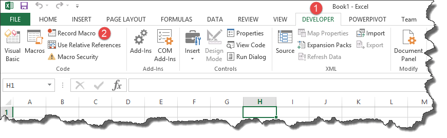
On the Developer tab, in the Code group, click Macros.
-
In the Macro name box, click the macro that you want to run, and press the Run button.
-
You also have other choices:
-
Options — Add a shortcut key, or a macro description.
-
Step — This will open the Visual Basic Editor to the first line of the macro. Pressing F8 will let you step through the macro code one line at a time.
-
Edit — This will open the Visual Basic Editor and let you edit the macro code as needed. Once you’ve made changes, you can press F5 to run the macro from the editor.
-
You can add a combination shortcut key to a macro when you record it, and you can also add one to an existing macro:
-
On the Developer tab, in the Code group, click Macros.
-
In the Macro name box, click the macro that you want to assign to a combination shortcut key.
-
Click Options.
The Macro Options dialog box appears.
-
In the Shortcut key box, type any lowercase or uppercase letter that you want to use with the shortcut key.
Notes:
-
For Windows, the shortcut key for lowercase letters is Ctrl+letter. For uppercase letters, it’s Ctrl+Shift+Letter.
-
For Mac, the shortcut key for lowercase letters is Option+Command+letter, but Ctrl+letter will work as well. For uppercase letters, it’s Ctrl+Shift+Letter.
-
Be careful assigning shortcut keys, because they will override any equivalent default Excel shortcut key while the workbook that contains the macro is open. For example, if you assign a macro to Ctrl+z, you’ll lose the ability to Undo. Because of this, it’s generally a good idea to use Ctrl+Shift+Uppercase letter instead, like Ctrl+Shift+Z, which doesn’t have an equivalent shortcut in Excel.
For a list of Ctrl combination shortcut keys that are already assigned in Excel, see the article Excel shortcut and function keys.
-
-
In the Description box, type a description of the macro.
-
Click OK to save your changes, and then click Cancel to close the Macro dialog box.
To run a macro from a button on the Quick Access toolbar, you first have to add the button to the toolbar. To do that, see Assign a macro to a button.
You can create a custom group that appears on a tab in the ribbon, and then assign a macro to a button in that group. For example, you can add a custom group named «My Macros» to the Developer tab, and then add a macro (that appears as a button) to the new group. To do that, see Assign a macro to a button.
Run a macro by clicking an area on a graphic object
You can create a hotspot on a graphic that users can click to run a macro.
-
In the worksheet, insert a graphic object, such as a picture, or draw a shape. A common scenario is to draw a Rounded Rectangle shape, and format it so it looks like a button.
To learn about inserting a graphic object, see Add, change, or delete shapes.
-
Right-click the hotspot that you created, and then click Assign Macro.
-
Do one of the following:
-
To assign an existing macro to the graphic object, double-click the macro or enter its name in the Macro name box.
-
To record a new macro to assign to the selected graphic object, click Record, type a name for the macro in the Record Macro dialog box, and then click OK to begin recording your macro. When you finish recording the macro, click Stop Recording
 on the Developer tab in the Code group.
Tip: You can also click Stop Recording
on the left side of the status bar. -
To edit an existing macro, click the name of the macro in the Macro name box, and then click Edit.
-
-
Click OK.
 on the Developer tab in the Code group.
On the Developer tab, click Visual Basic to launch the Visual Basic Editor (VBE). Browse the Project Explorer to the module that contains the macro you want to run, and open it. All of the macros in that module will be listed in the pane on the right. Select the macro you want to run, by placing your cursor anywhere within the macro, and press F5, or on the menu, go to Run > Run Macro.
Create a Workbook_Open event.
The following example uses the Open event to run a macro when you open the workbook.
-
Open the workbook where you want to add the macro, or create a new workbook.
-
On the Developer tab, in the Code group, click Visual Basic.
-
In the Project Explorer window, right-click the ThisWorkbook object, and then click View Code.
Tip: If the Project Explorer window is not visible, on the View menu, click Project Explorer.
-
In the Object list above the Code window, select Workbook.
This automatically creates an empty procedure for the Open event, such as this:
Private Sub Workbook_Open()
End Sub
-
Add the following lines of code to the procedure:
Private Sub Workbook_Open()
MsgBox Date
Worksheets(«Sheet1»).Range(«A1»).Value = Date
End Sub -
Switch to Excel and save the workbook as a macro-enabled workbook (.xlsm).
-
Close and reopen the workbook. When you open the workbook again, Excel runs the Workbook_Open procedure, which displays today’s date in a message box.
-
Click OK in the message box.
Note: The cell A1 on Sheet1 also contains the date as a result of running the Workbook_Open procedure.
Need more help?
You can always ask an expert in the Excel Tech Community or get support in the Answers community.
Top of Page
See Also
Automatically run a macro when opening a workbook
Automate tasks with the Macro Recorder
Record a macro to open specific workbooks when Excel starts
Create and save all your macros in a single workbook
Save a macro
Need more help?
Want more options?
Explore subscription benefits, browse training courses, learn how to secure your device, and more.
Communities help you ask and answer questions, give feedback, and hear from experts with rich knowledge.
![]()
Download Article
![]()
Download Article
This wikiHow teaches you how to enable, create, run, and save macros in Microsoft Excel. Macros are miniature programs which allow you to perform complex tasks, such as calculating formulas or creating charts, within Excel. Macros can save significant amounts of time when applied to repetitive tasks, and thanks to Excel’s «Record Macro» feature, you don’t have to know anything about programming in order to create a macro.
Things You Should Know
- Macros make it easy to automatic tasks in Microsoft Excel.
- To create macros yourself, you’ll need to enable macros in the Developer menu of Excel.
- Saving a macro-enabled spreadsheet is a little different than saving a spreadsheet without macros.
-
1
Open Excel. Double-click the Excel app icon, which resembles a white «X» on a green box, then click Blank workbook.
- If you have a specific file which you want to open in Excel, double-click that file to open it instead.
-
2
Click File. It’s in the upper-left side of the Excel window.
- On a Mac, click Excel in the upper-left corner of the screen to prompt a drop-down menu.
Advertisement
-
3
Click Options. You’ll find this on the left side of the Excel window.
- On a Mac, you’ll click Preferences… in the drop-down menu.
-
4
Click Customize Ribbon. It’s on the left side of the Excel Options window.[1]
- On a Mac, click instead Ribbon & Toolbar in the Preferences window.
-
5
Check the «Developer» box. This box is near the bottom of the «Main Tabs» list of options.
-
6
Click OK. It’s at the bottom of the window. You can now use macros in Excel.
- On a Mac, you’ll click Save here instead.


Advertisement
-
1
Enter any necessary data. If you opened a blank workbook, enter any data which you want to use before proceeding.
- You can also close Excel and open a specific Excel file by double-clicking it.
-
2
Click the Developer tab. It’s at the top of the Excel window. Doing so opens a toolbar here.
-
3
Click Record Macro. It’s in the toolbar. A pop-up window will appear.
-
4
Enter a name for the macro. In the «Macro name» text box, type in the name for your macro. This will help you identify the macro later.
-
5
Create a shortcut key combination if you like. Press the ⇧ Shift key along with another letter key (e.g., the E key) to create the keyboard shortcut. You can use this keyboard shortcut to run the macro later.
- On a Mac, the shortcut key combination will end up being ⌥ Option+⌘ Command and your key (e.g., ⌥ Option+⌘ Command+T).
-
6
Click the «Store macro in» drop-down box. It’s in the middle of the window. Doing so prompts a drop-down menu.
-
7
Click This Workbook. This option is in the drop-down menu. Your macro will be stored inside your spreadsheet, making it possible for anyone who has the spreadsheet to access the macro.
-
8
Click OK. It’s at the bottom of the window. Doing this saves your macro settings and begins recording.
-
9
Perform the macro’s steps. Any step you perform between clicking OK and clicking Stop Recording while be added to the macro. For example, if you wanted to create a macro which turns two columns’ worth of data into a chart, you would do the following:
- Click and drag your mouse across the data to select it.
- Click Insert
- Select a chart shape.
- Click the chart that you want to use.
-
10
Click Stop Recording. It’s in the Developer toolbar. This will save your macro.


Advertisement
-
1
Understand why you have to save the spreadsheet with macros enabled. If you don’t save your spreadsheet as a macro-enabled spreadsheet (XLSM format), the macro won’t be saved as part of the spreadsheet, meaning that other people on different computers won’t be able to use your macro if you send the workbook to them.
-
2
Click File. It’s in the upper-left corner of the Excel window (Windows) or the screen (Mac). Doing so will prompt a drop-down menu.
-
3
Click Save As. This option is on the left side of the window (Windows) or in the drop-down menu (Mac).
-
4
Double-click This PC. It’s in the column of save locations near the left side of the window. A «Save As» window will open.
- Skip this step on a Mac.
-
5
Enter a name for your Excel file. In the «Name» text box, type in the name for your Excel spreadsheet.
-
6
Change the file format to XLSM. Click the «Save as type» drop-down box, then click Excel Macro-Enabled Workbook in the resulting drop-down menu.[2]
- On a Mac, you’ll replace the «xlsx» at the end of the file’s name with xlsm.
-
7
Select a save location. Click a folder in which you want to save the Excel file (e.g., Desktop).
- On a Mac, you must first click the «Where» drop-down box.
-
8
Click Save. It’s at the bottom of the window. Doing so will save your Excel spreadsheet to your selected location, and your macro will be saved along with it.


Advertisement
-
1
Open the macro-enabled spreadsheet. Double-click the spreadsheet that has the macro in it to open the spreadsheet in Excel.
-
2
Click Enable Content. It’s in a yellow bar at the top of the Excel window. This will unlock the spreadsheet and allow you to use the macro.
- If you don’t see this option, skip this step.
-
3
Click the Developer tab. This option is at the top of the Excel window.
- You can also just press the key combination you set for the macro. If you do so, the macro will run, and you can skip the rest of this method.
-
4
Click Macros. You’ll find it in the Developer tab’s toolbar. A pop-up window will open.
-
5
Select your macro. Click the name of the macro which you want to run.
-
6
Click Run. It’s on the right side of the window. Your macro will begin running.
-
7
Wait for the macro to finish running. Depending on how large your macro is, this can take several seconds.


Advertisement
Add New Question
-
Question
Can I use a macro that I create in other spreadsheets and future spreadsheets on the same pc?

Yes, you can use a macro that you crate in other spreadsheets and future spreadsheets on the same pc.
-
Question
How can I write macros that will change a spreadsheet as soon as I create it?
You will first need a basic understanding of VBA. There are many tutorials on this.
Ask a Question
200 characters left
Include your email address to get a message when this question is answered.
Submit
Advertisement
Video
-
Macros are generally useful for automating tasks which you must perform often, such as calculating payroll at the end of the week.
Thanks for submitting a tip for review!
Advertisement
-
Although most macros are benign, some macros can maliciously change or delete information on your computer. Never open a macro from a source which you don’t trust.
Advertisement
About This Article
Article SummaryX
1. Enable Developer options in Excel.
2. Click the Developer tab.
3. Click Record Macro.
4. Enter the macro name and details.
5. Click OK.
6. Perform the macro’s steps.
7. Click Stop Recording.
Did this summary help you?
Thanks to all authors for creating a page that has been read 710,423 times.
Is this article up to date?
Excel Macro is a record and playback tool that simply records your Excel steps and the macro will play it back as many times as you want. VBA Macros save time as they automate repetitive tasks. It is a piece of programming code that runs in an Excel environment but you don’t need to be a coder to program macros. Though, you need basic knowledge of VBA to make advanced modifications in the macro.
In this Macros in Excel for beginners tutorial, you will learn Excel macro basics:
- What is an Excel Macro?
- Why are Excel Macros Used in Excel?
- What is VBA in a Layman’s Language?
- Excel Macro Basics
- Step by Step Example of Recording Macros in Excel
Why are Excel Macros Used in Excel?
As humans, we are creatures of habit. There are certain things that we do on a daily basis, every working day. Wouldn’t it be better if there were some magical way of pressing a single button and all of our routine tasks are done? I can hear you say yes. Macro in Excel helps you to achieve that. In a layman’s language, a macro is defined as a recording of your routine steps in Excel that you can replay using a single button.
For example, you are working as a cashier for a water utility company. Some of the customers pay through the bank and at the end of the day, you are required to download the data from the bank and format it in a manner that meets your business requirements.
You can import the data into Excel and format. The following day you will be required to perform the same ritual. It will soon become boring and tedious. Macros solve such problems by automating such routine tasks. You can use a macro to record the steps of
- Importing the data
- Formatting it to meet your business reporting requirements.
What is VBA in a Layman’s Language?
VBA is the acronym for Visual Basic for Applications. It is a programming language that Excel uses to record your steps as you perform routine tasks. You do not need to be a programmer or a very technical person to enjoy the benefits of macros in Excel. Excel has features that automatically generated the source code for you. Read the article on VBA for more details.
Excel Macro Basics
Macros are one of the developer features. By default, the tab for developers is not displayed in Excel. You will need to display it via customize report
Excel Macros can be used to compromise your system by attackers. By default, they are disabled in Excel. If you need to run macros, you will need to enable running macros and only run macros that you know come from a trusted source
If you want to save Excel macros, then you must save your workbook in a macro-enabled format *.xlsm
The macro name should not contain any spaces.
Always fill in the description of the macro when creating one. This will help you and others to understand what the macro is doing.
Step by Step Example of Recording Macros in Excel
Now in this Excel macros tutorial, we will learn how to create a macro in Excel:
We will work with the scenario described in the importance of macros Excel. For this Excel macro tutorial, we will work with the following CSV file to write macros in Excel.

You can download the above file here
Download the above CSV File & Macros
We will create a macro enabled template that will import the above data and format it to meet our business reporting requirements.
Enable Developer Option
To execute VBA program, you have to have access to developer option in Excel. Enable the developer option as shown in the below Excel macro example and pin it into your main ribbon in Excel.
Step 1)Go to main menu “FILE”
Select option “Options.”


Step 2) Now another window will open, in that window do following things
- Click on Customize Ribbon
- Mark the checker box for Developer option
- Click on OK button

Step 3) Developer Tab
You will now be able to see the DEVELOPER tab in the ribbon

Step 4) Download CSV
First, we will see how we can create a command button on the spreadsheet and execute the program.
- Create a folder in drive C named Bank Receipts
- Paste the receipts.csv file that you downloaded

Step 5) Record Macro
- Click on the DEVELOPER tab
- Click on Record Macro as shown in the image below
You will get the following dialogue window

- Enter ImportBankReceipts as the macro name.
- Step two will be there by default
- Enter the description as shown in the above diagram
- Click on “OK” tab
Step 6) Perform Macro Operations/Steps you want to record
- Put the cursor in cell A1
- Click on the DATA tab
- Click on From Text button on the Get External data ribbon bar
You will get the following dialogue window

- Go to the local drive where you have stored the CSV file
- Select the CSV file
- Click on Import button
You will get the following wizard

Click on Next button after following the above steps

Follow the above steps and click on next button

- Click on Finish button
- Your workbook should now look as follows

Step 7) Format the Data
Make the columns bold, add the grand total and use the SUM function to get the total amount.

Step  Stop Recording Macro
Now that we have finished our routine work, we can click on stop recording macro button as shown in the image below

Step 9) Replay the Macro
Before we save our work book, we will need to delete the imported data. We will do this to create a template that we will be copying every time we have new receipts and want to run the ImportBankReceipts macro.
- Highlight all the imported data
- Right click on the highlighted data
- Click on Delete
- Click on save as button
- Save the workbook in a macro enabled format as shown below

- Make a copy of the newly saved template
- Open it
- Click on DEVELOPER tab
- Click on Macros button
You will get the following dialogue window

- Select ImportBankReceipts
- Highlights the description of your macro
- Click on Run button
You will get the following data

Congratulations, you just created your first macro in Excel.
Summary
Macros simplify our work lives by automating most of the routine works that we do. Macros Excel are powered by Visual Basic for Applications.
#Руководства
- 23 май 2022
-
0
Как с помощью макросов автоматизировать рутинные задачи в Excel? Какие команды они выполняют? Как создать макрос новичку? Разбираемся на примере.
Иллюстрация: Meery Mary для Skillbox Media

Рассказывает просто о сложных вещах из мира бизнеса и управления. До редактуры — пять лет в банке и три — в оценке имущества. Разбирается в Excel, финансах и корпоративной жизни.
Макрос (или макрокоманда) в Excel — алгоритм действий в программе, который объединён в одну команду. С помощью макроса можно выполнить несколько шагов в Excel, нажав на одну кнопку в меню или на сочетание клавиш.
Обычно макросы используют для автоматизации рутинной работы — вместо того чтобы выполнять десяток повторяющихся действий, пользователь записывает одну команду и затем запускает её, когда нужно совершить эти действия снова.
Например, если нужно добавить название компании в несколько десятков документов и отформатировать его вид под корпоративный дизайн, можно делать это в каждом документе отдельно, а можно записать ход действий при создании первого документа в макрос — и затем применить его ко всем остальным. Второй вариант будет гораздо проще и быстрее.
В статье разберёмся:
- как работают макросы и как с их помощью избавиться от рутины в Excel;
- какие способы создания макросов существуют и как подготовиться к их записи;
- как записать и запустить макрос начинающим пользователям — на примере со скриншотами.
Общий принцип работы макросов такой:
- Пользователь записывает последовательность действий, которые нужно выполнить в Excel, — о том, как это сделать, поговорим ниже.
- Excel обрабатывает эти действия и создаёт для них одну общую команду. Получается макрос.
- Пользователь запускает этот макрос, когда ему нужно выполнить эту же последовательность действий ещё раз. При записи макроса можно задать комбинацию клавиш или создать новую кнопку на главной панели Excel — если нажать на них, макрос запустится автоматически.
Макросы могут выполнять любые действия, которые в них запишет пользователь. Вот некоторые команды, которые они умеют делать в Excel:
- Автоматизировать повторяющиеся процедуры.
Например, если пользователю нужно каждый месяц собирать отчёты из нескольких файлов в один, а порядок действий каждый раз один и тот же, можно записать макрос и запускать его ежемесячно.
- Объединять работу нескольких программ Microsoft Office.
Например, с помощью одного макроса можно создать таблицу в Excel, вставить и сохранить её в документе Word и затем отправить в письме по Outlook.
- Искать ячейки с данными и переносить их в другие файлы.
Этот макрос пригодится, когда нужно найти информацию в нескольких объёмных документах. Макрос самостоятельно отыщет её и принесёт в заданный файл за несколько секунд.
- Форматировать таблицы и заполнять их текстом.
Например, если нужно привести несколько таблиц к одному виду и дополнить их новыми данными, можно записать макрос при форматировании первой таблицы и потом применить его ко всем остальным.
- Создавать шаблоны для ввода данных.
Команда подойдёт, когда, например, нужно создать анкету для сбора данных от сотрудников. С помощью макроса можно сформировать такой шаблон и разослать его по корпоративной почте.
- Создавать новые функции Excel.
Если пользователю понадобятся дополнительные функции, которых ещё нет в Excel, он сможет записать их самостоятельно. Все базовые функции Excel — это тоже макросы.
Все перечисленные команды, а также любые другие команды пользователя можно комбинировать друг с другом и на их основе создавать макросы под свои потребности.
В Excel и других программах Microsoft Office макросы создаются в виде кода на языке программирования VBA (Visual Basic for Applications). Этот язык разработан в Microsoft специально для программ компании — он представляет собой упрощённую версию языка Visual Basic. Но это не значит, что для записи макроса нужно уметь кодить.
Есть два способа создания макроса в Excel:
- Написать макрос вручную.
Это способ для продвинутых пользователей. Предполагается, что они откроют окно Visual Basic в Еxcel и самостоятельно напишут последовательность действий для макроса в виде кода.
- Записать макрос с помощью кнопки меню Excel.
Способ подойдёт новичкам. В этом варианте Excel запишет программный код вместо пользователя. Нужно нажать кнопку записи и выполнить все действия, которые планируется включить в макрос, и после этого остановить запись — Excel переведёт каждое действие и выдаст алгоритм на языке VBA.
Разберёмся на примере, как создать макрос с помощью второго способа.
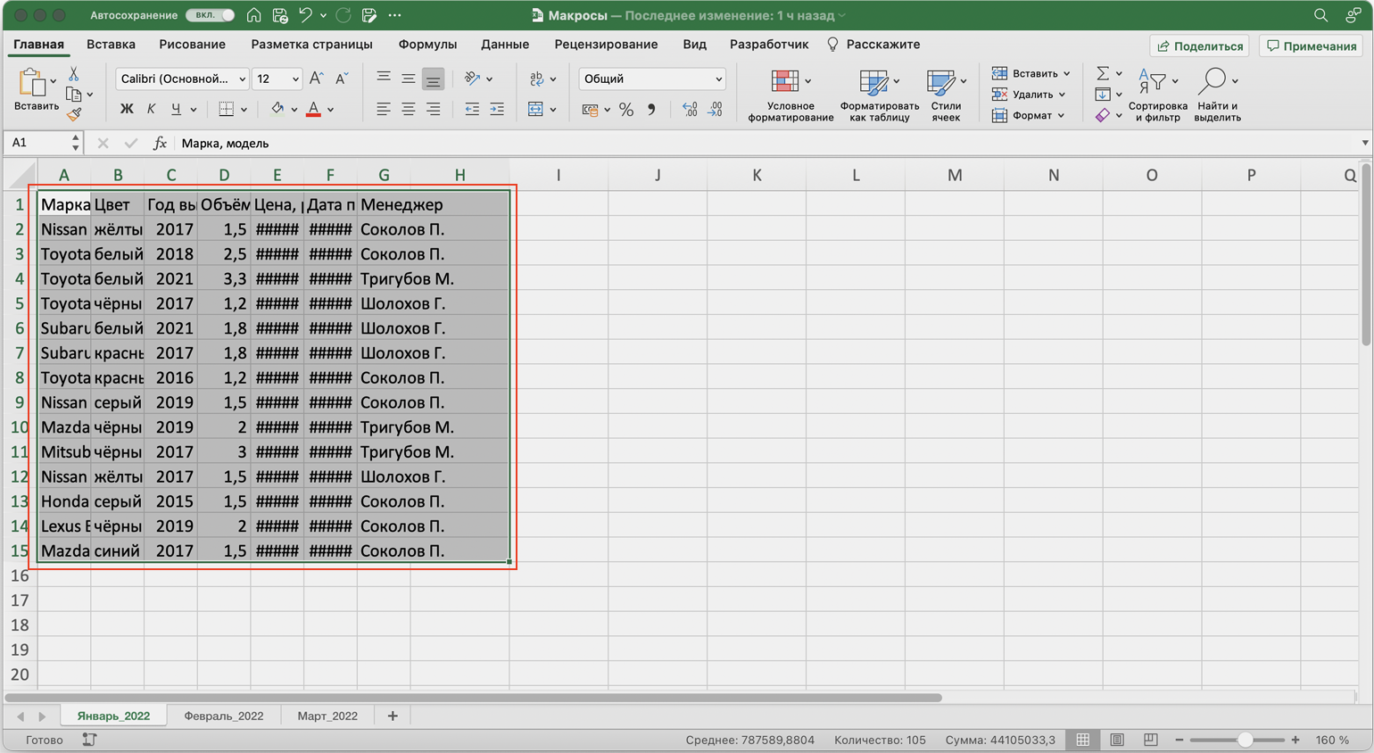
Допустим, специальный сервис автосалона выгрузил отчёт по продажам за три месяца первого квартала в формате таблиц Excel. Эти таблицы содержат всю необходимую информацию, но при этом никак не отформатированы: колонки слиплись друг с другом и не видны полностью, шапка таблицы не выделена и сливается с другими строками, часть данных не отображается.
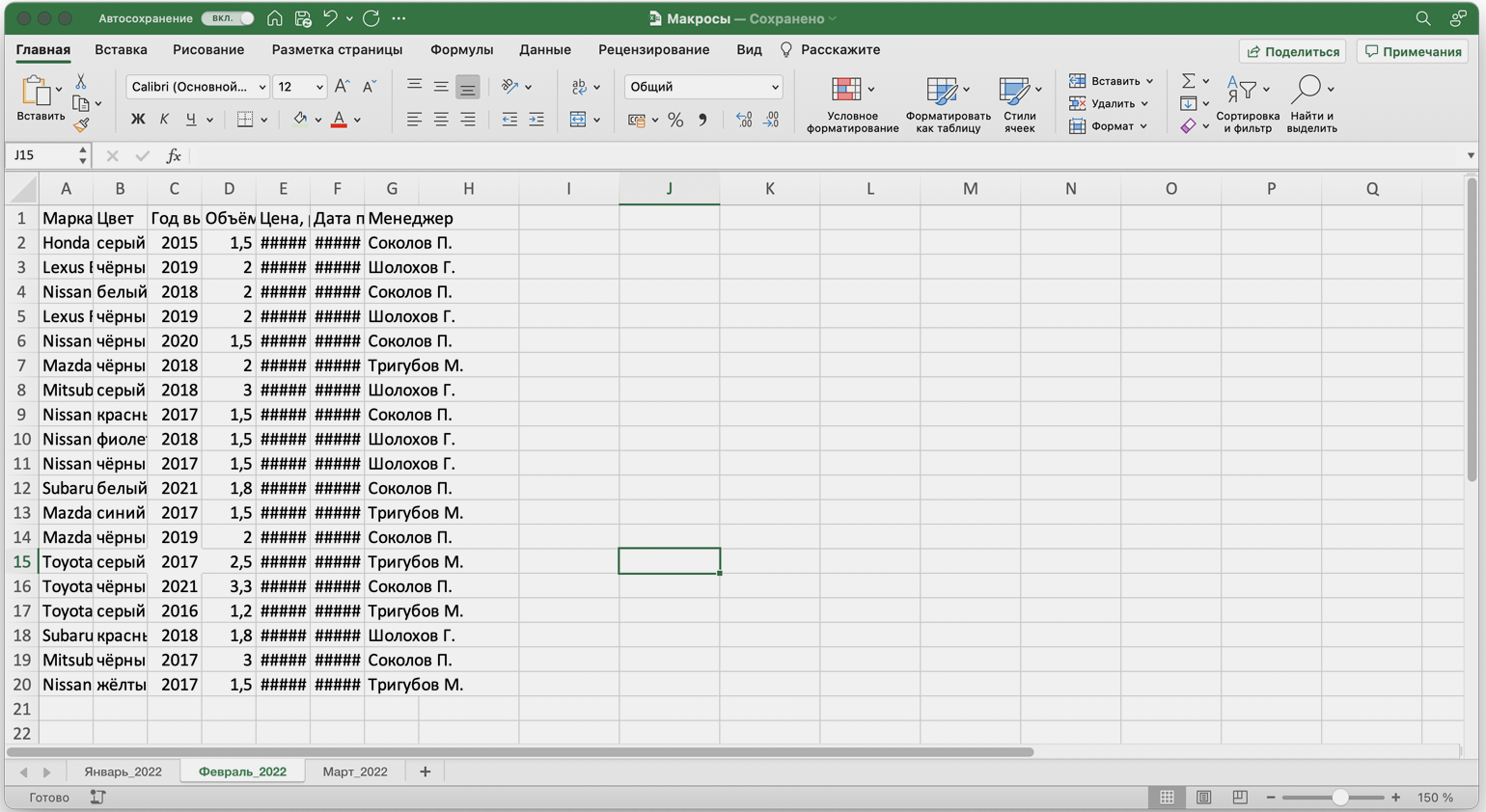
Скриншот: Skillbox Media
Пользоваться таким отчётом неудобно — нужно сделать его наглядным. Запишем макрос при форматировании таблицы с продажами за январь и затем применим его к двум другим таблицам.
Готовимся к записи макроса
Кнопки для работы с макросами в Excel находятся во вкладке «Разработчик». Эта вкладка по умолчанию скрыта, поэтому для начала разблокируем её.
В операционной системе Windows это делается так: переходим во вкладку «Файл» и выбираем пункты «Параметры» → «Настройка ленты». В открывшемся окне в разделе «Основные вкладки» находим пункт «Разработчик», отмечаем его галочкой и нажимаем кнопку «ОК» → в основном меню Excel появляется новая вкладка «Разработчик».
В операционной системе macOS это нужно делать по-другому. В самом верхнем меню нажимаем на вкладку «Excel» и выбираем пункт «Параметры…».
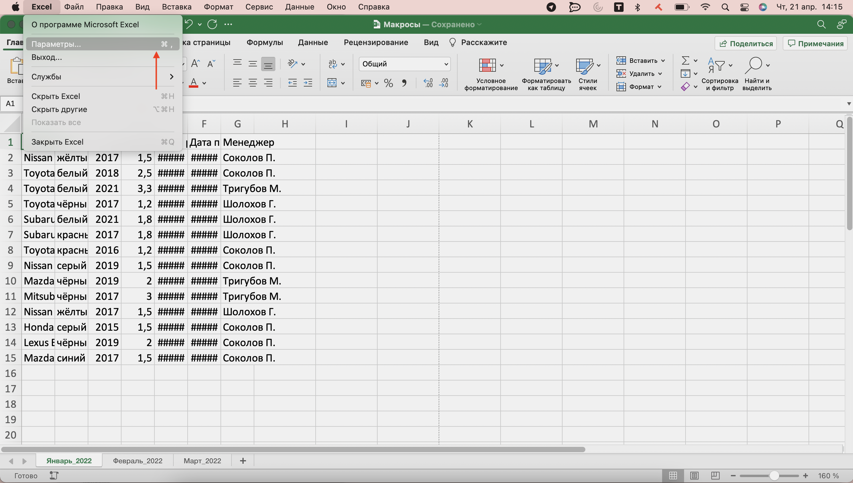
Скриншот: Skillbox Media
В появившемся окне нажимаем кнопку «Лента и панель».
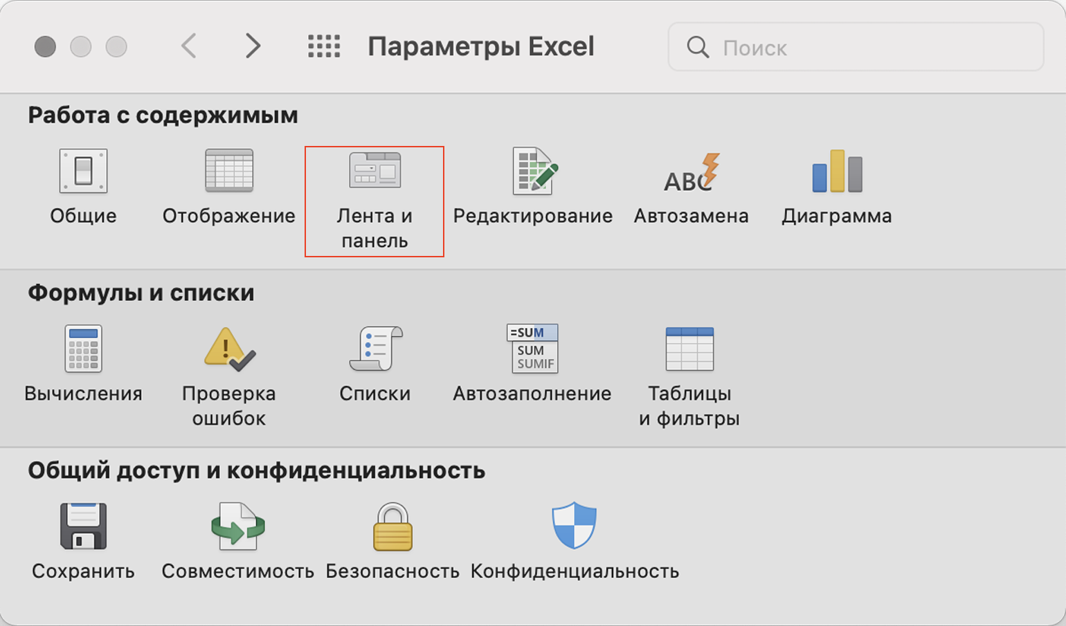
Скриншот: Skillbox Media
Затем в правой панели «Настроить ленту» ищем пункт «Разработчик» и отмечаем его галочкой. Нажимаем «Сохранить».
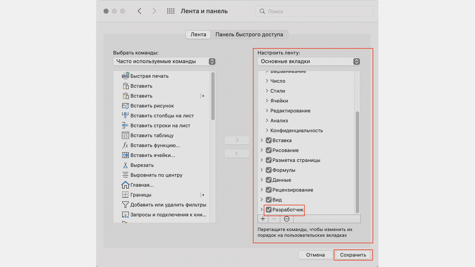
Скриншот: Skillbox Media
Готово — вкладка «Разработчик» появилась на основной панели Excel.
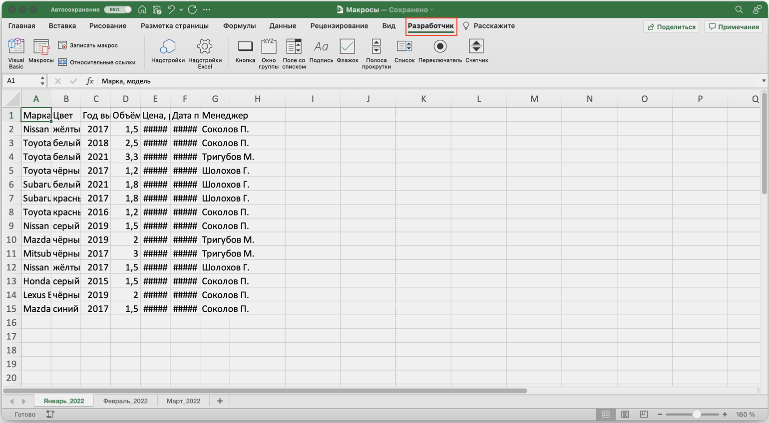
Скриншот: Skillbox Media
Чтобы Excel смог сохранить и в дальнейшем использовать макрос, нужно пересохранить документ в формате, который поддерживает макросы. Это делается через команду «Сохранить как» на главной панели. В появившемся меню нужно выбрать формат «Книга Excel с поддержкой макросов».
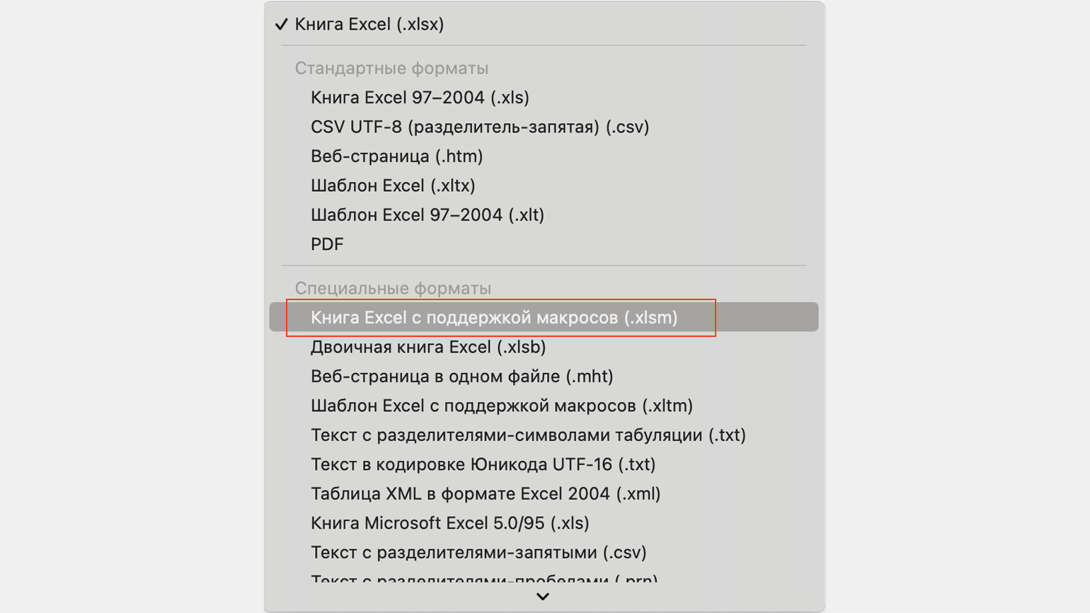
Скриншот: Skillbox Media
Перед началом записи макроса важно знать об особенностях его работы:
- Макрос записывает все действия пользователя.
После старта записи макрос начнёт регистрировать все клики мышки и все нажатия клавиш. Поэтому перед записью последовательности лучше хорошо отработать её, чтобы не добавлять лишних действий и не удлинять код. Если требуется записать длинную последовательность задач — лучше разбить её на несколько коротких и записать несколько макросов.
- Работу макроса нельзя отменить.
Все действия, которые выполняет запущенный макрос, остаются в файле навсегда. Поэтому перед тем, как запускать макрос в первый раз, лучше создать копию всего файла. Если что-то пойдёт не так, можно будет просто закрыть его и переписать макрос в созданной копии.
- Макрос выполняет свой алгоритм только для записанного диапазона таблиц.
Если при записи макроса пользователь выбирал диапазон таблицы, то и при запуске макроса в другом месте он выполнит свой алгоритм только в рамках этого диапазона. Если добавить новую строку, макрос к ней применяться не будет. Поэтому при записи макроса можно сразу выбирать большее количество строк — как это сделать, показываем ниже.
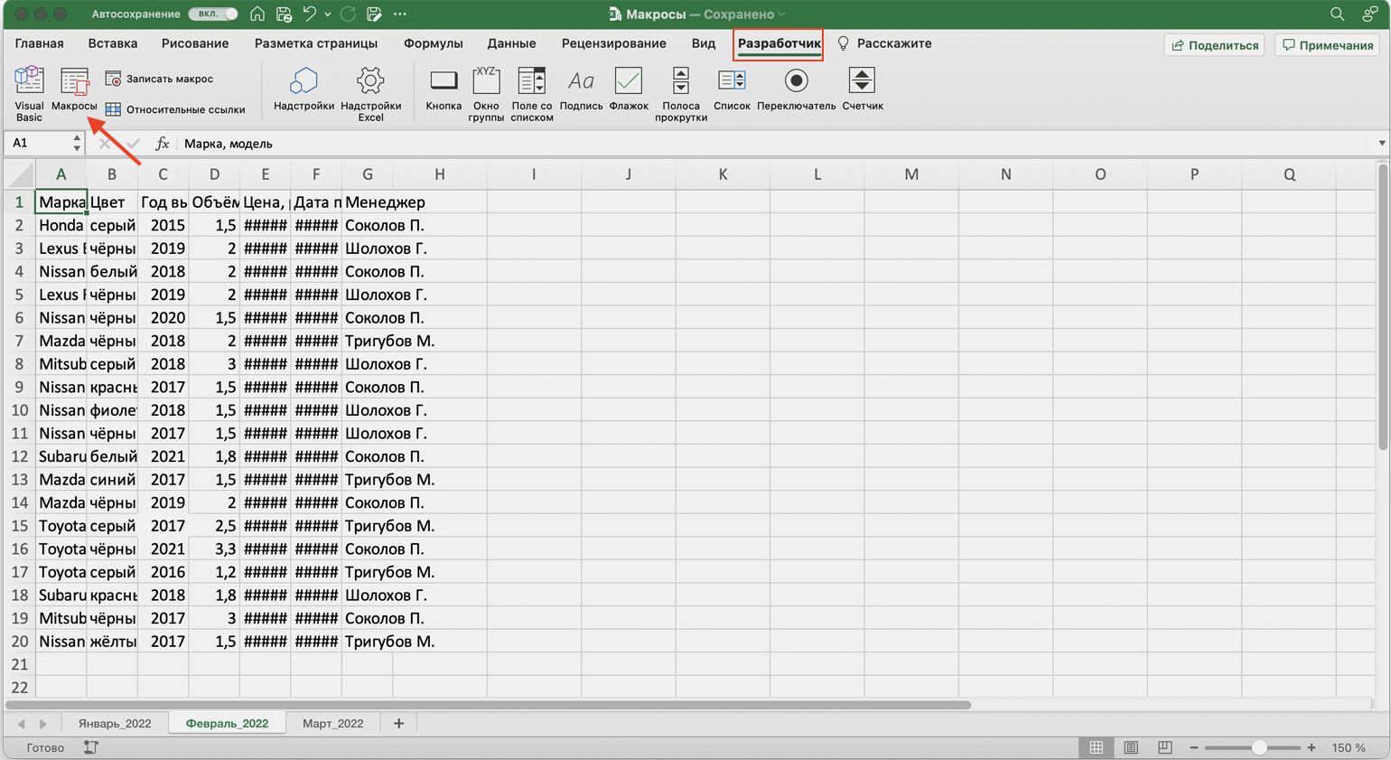
Для начала записи макроса перейдём на вкладку «Разработчик» и нажмём кнопку «Записать макрос».
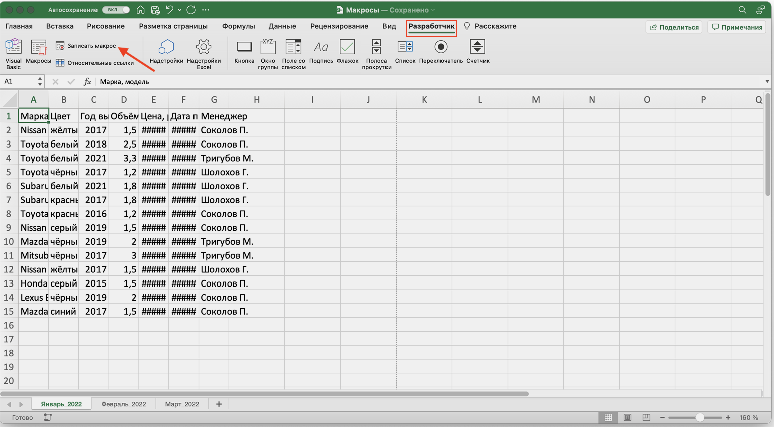
Скриншот: Skillbox Media
Появляется окно для заполнения параметров макроса. Нужно заполнить поля: «Имя макроса», «Сохранить в», «Сочетание клавиш», «Описание».
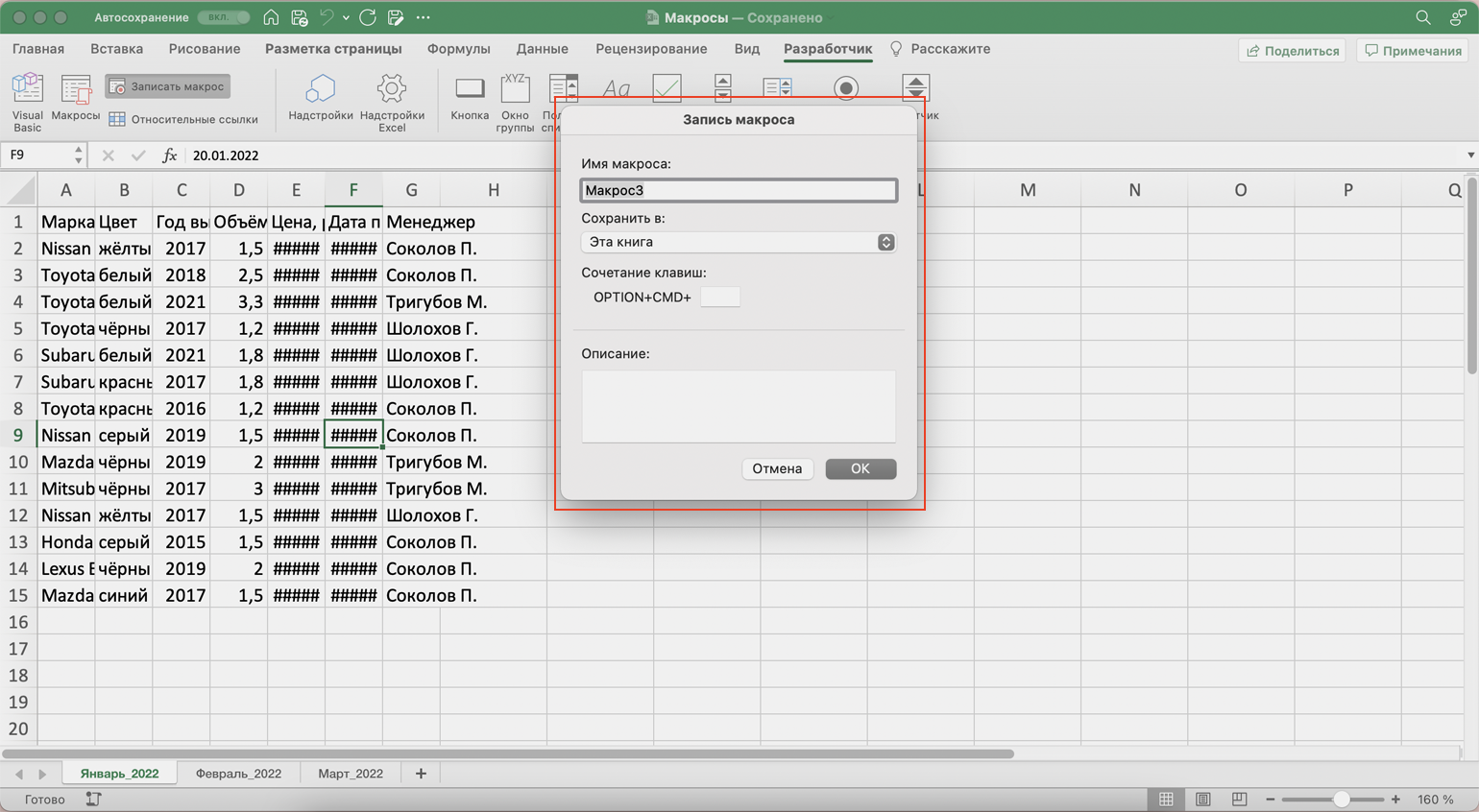
Скриншот: Skillbox Media
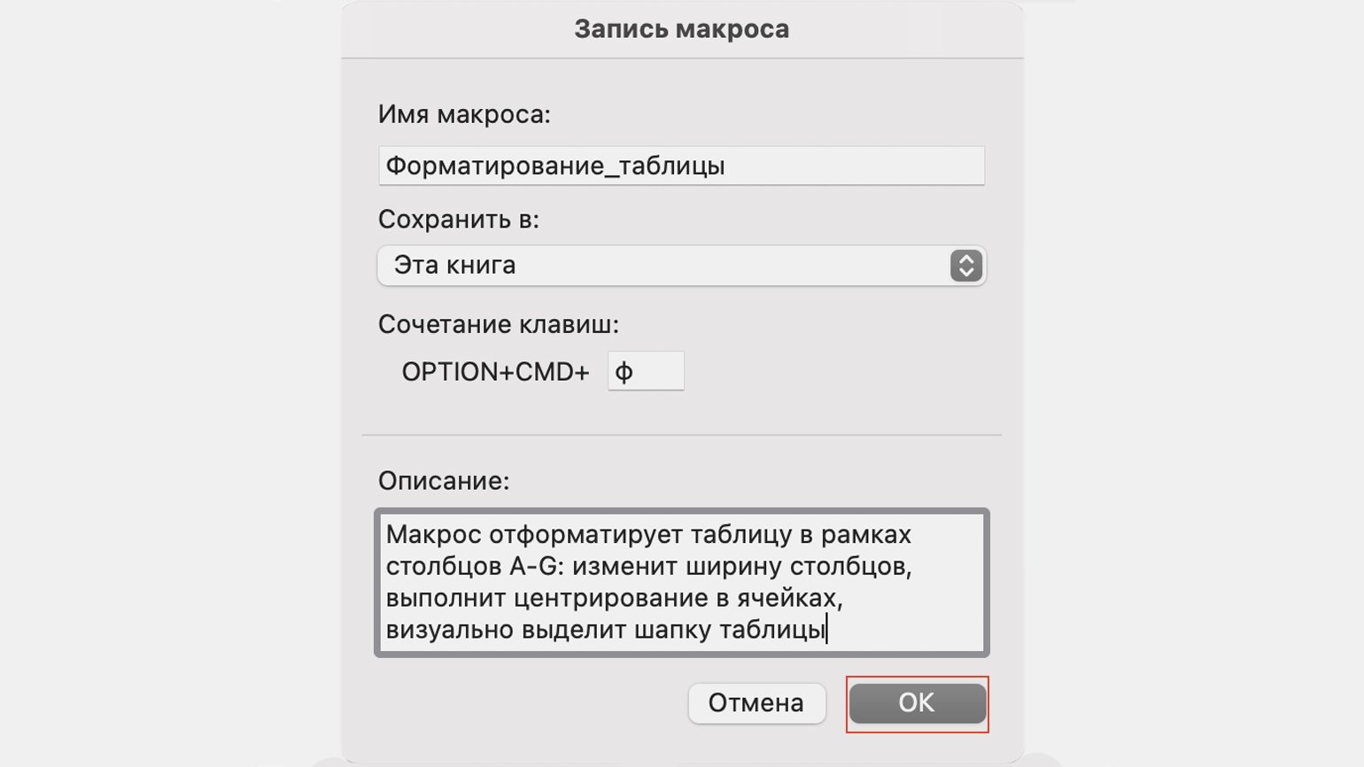
«Имя макроса» — здесь нужно придумать и ввести название для макроса. Лучше сделать его логически понятным, чтобы в дальнейшем можно было быстро его найти.
Первым символом в названии обязательно должна быть буква. Другие символы могут быть буквами или цифрами. Важно не использовать пробелы в названии — их можно заменить символом подчёркивания.
«Сохранить в» — здесь нужно выбрать книгу, в которую макрос сохранится после записи.
Если выбрать параметр «Эта книга», макрос будет доступен при работе только в этом файле Excel. Чтобы макрос был доступен всегда, нужно выбрать параметр «Личная книга макросов» — Excel создаст личную книгу макросов и сохранит новый макрос в неё.
«Сочетание клавиш» — здесь к уже выбранным двум клавишам (Ctrl + Shift в системе Windows и Option + Cmd в системе macOS) нужно добавить третью клавишу. Это должна быть строчная или прописная буква, которую ещё не используют в других быстрых командах компьютера или программы Excel.
В дальнейшем при нажатии этих трёх клавиш записанный макрос будет запускаться автоматически.
«Описание» — необязательное поле, но лучше его заполнять. Например, можно ввести туда последовательность действий, которые планируется записать в этом макросе. Так не придётся вспоминать, какие именно команды выполнит этот макрос, если нужно будет запустить его позже. Плюс будет проще ориентироваться среди других макросов.
В нашем случае с форматированием таблицы заполним поля записи макроса следующим образом и нажмём «ОК».
Скриншот: Skillbox Media
После этого начнётся запись макроса — в нижнем левом углу окна Excel появится значок записи.
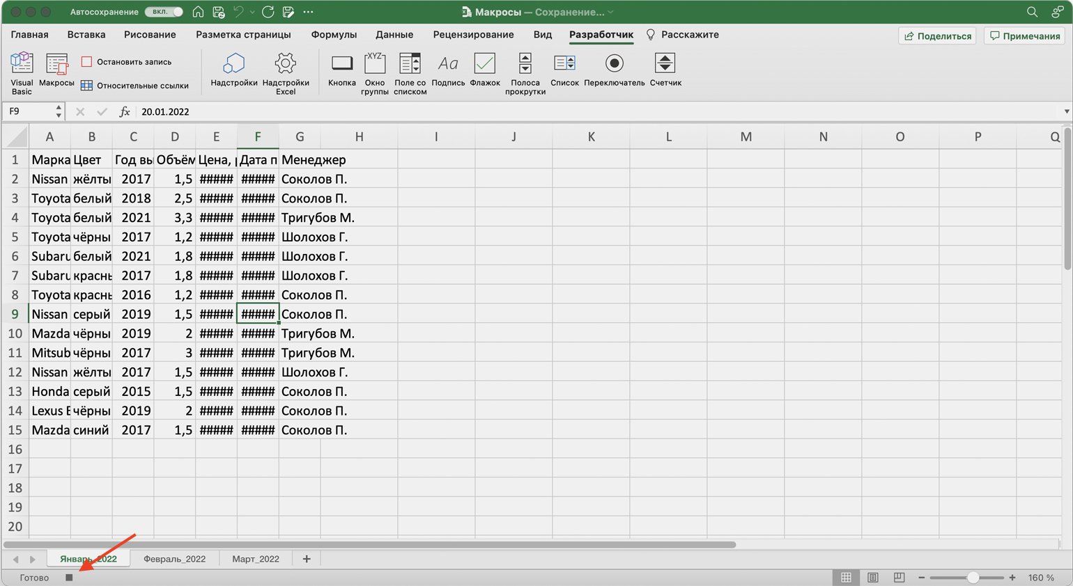
Скриншот: Skillbox Media
Пока идёт запись, форматируем таблицу с продажами за январь: меняем ширину всех столбцов, данные во всех ячейках располагаем по центру, выделяем шапку таблицы цветом и жирным шрифтом, рисуем границы.
Важно: в нашем случае у таблиц продаж за январь, февраль и март одинаковое количество столбцов, но разное количество строк. Чтобы в случае со второй и третьей таблицей макрос сработал корректно, при форматировании выделим диапазон так, чтобы в него попали не только строки самой таблицы, но и строки ниже неё. Для этого нужно выделить столбцы в строке с их буквенным обозначением A–G, как на рисунке ниже.
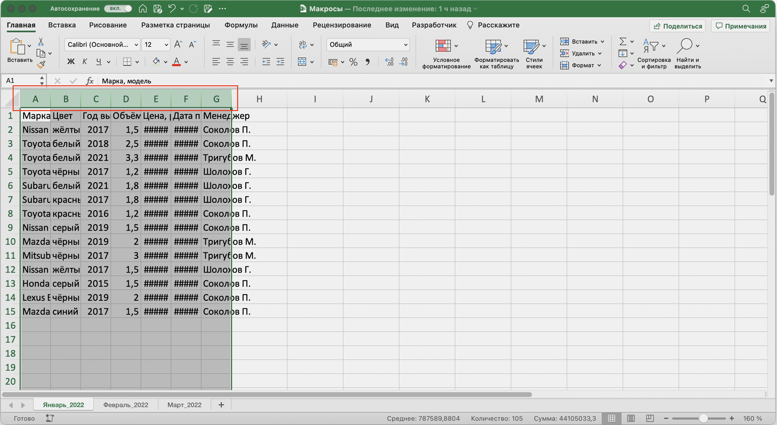
Скриншот: Skillbox Media
Если выбрать диапазон только в рамках первой таблицы, то после запуска макроса в таблице с большим количеством строк она отформатируется только частично.
Скриншот: Skillbox Media
После всех манипуляций с оформлением таблица примет такой вид:
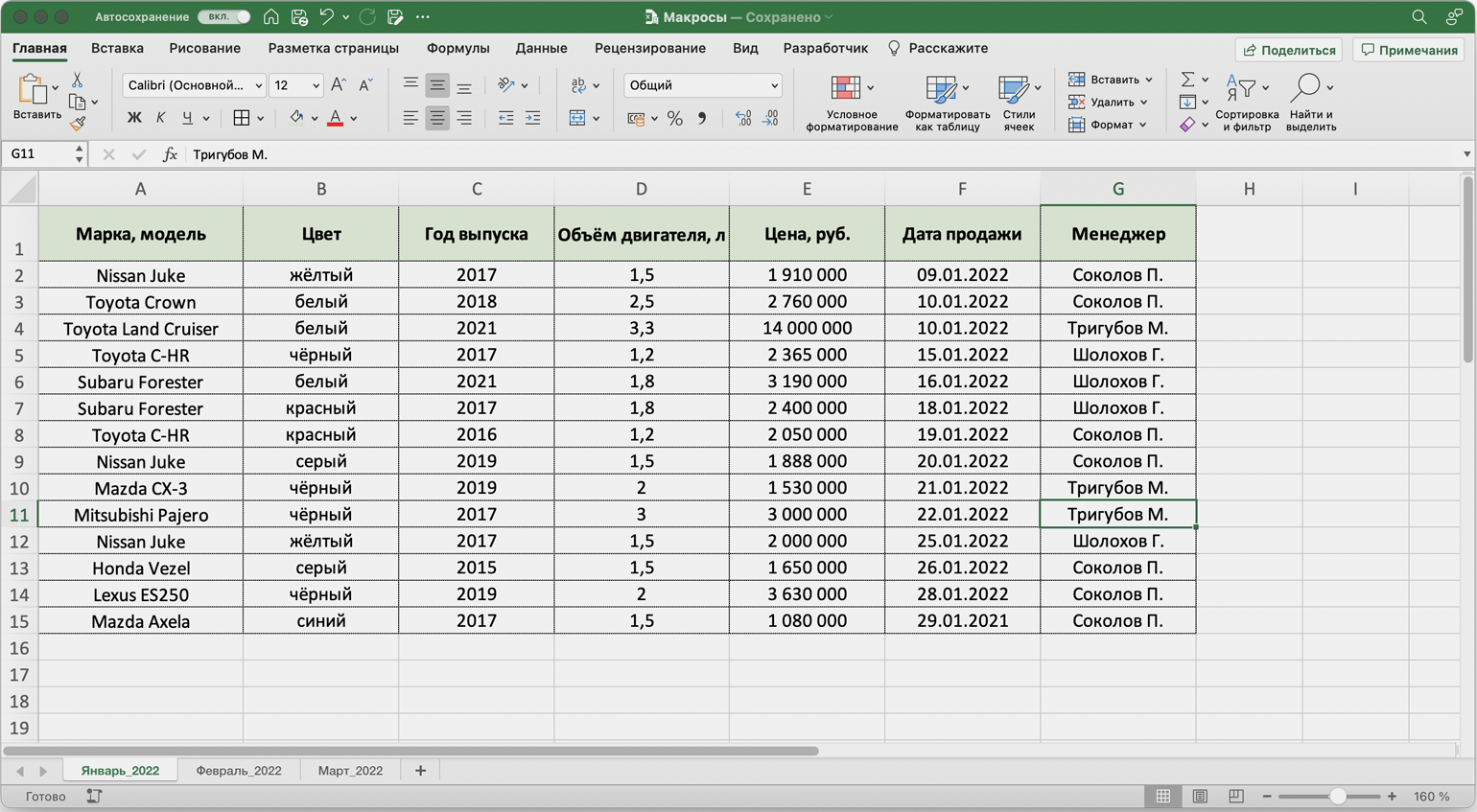
Скриншот: Skillbox Media
Проверяем, все ли действия с таблицей мы выполнили, и останавливаем запись макроса. Сделать это можно двумя способами:
- Нажать на кнопку записи в нижнем левом углу.
- Перейти во вкладку «Разработчик» и нажать кнопку «Остановить запись».
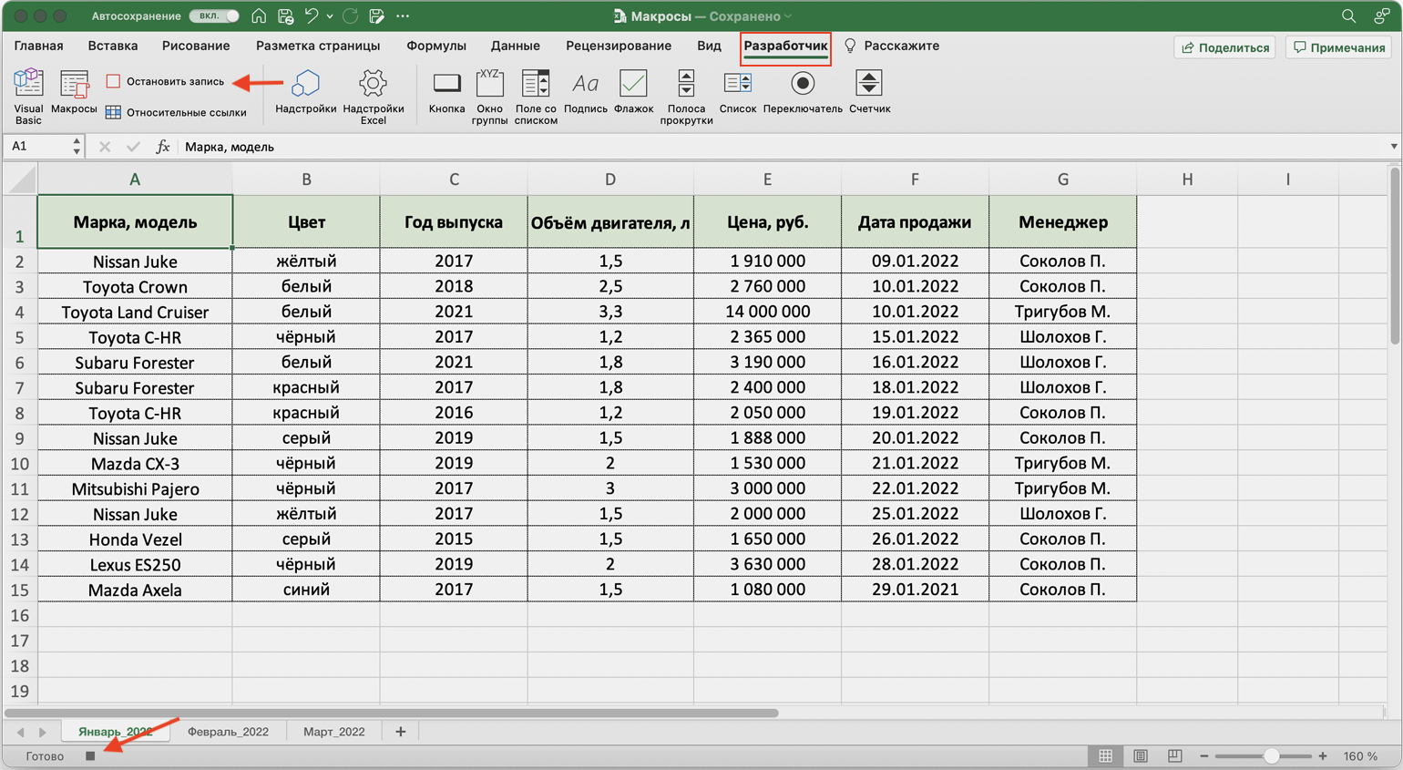
Скриншот: Skillbox Media
Готово — мы создали макрос для форматирования таблиц в границах столбцов A–G. Теперь его можно применить к другим таблицам.
Запускаем макрос
Перейдём в лист со второй таблицей «Февраль_2022». В первоначальном виде она такая же нечитаемая, как и первая таблица до форматирования.
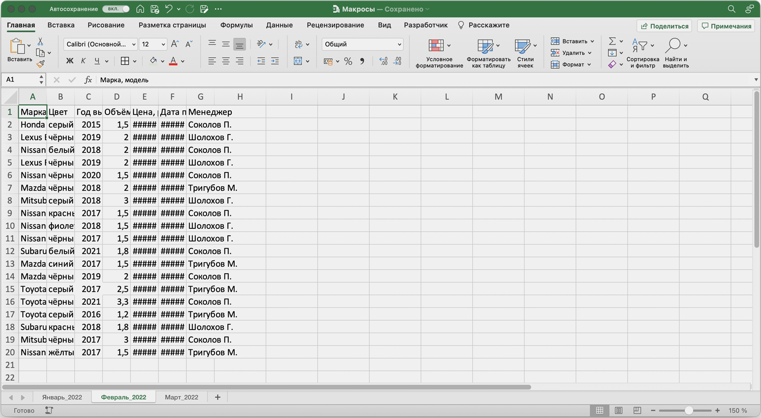
Скриншот: Skillbox Media
Отформатируем её с помощью записанного макроса. Запустить макрос можно двумя способами:
- Нажать комбинацию клавиш, которую выбрали при заполнении параметров макроса — в нашем случае Option + Cmd + Ф.
- Перейти во вкладку «Разработчик» и нажать кнопку «Макросы».
Скриншот: Skillbox Media
Появляется окно — там выбираем макрос, который нужно запустить. В нашем случае он один — «Форматирование_таблицы». Под ним отображается описание того, какие действия он включает. Нажимаем «Выполнить».
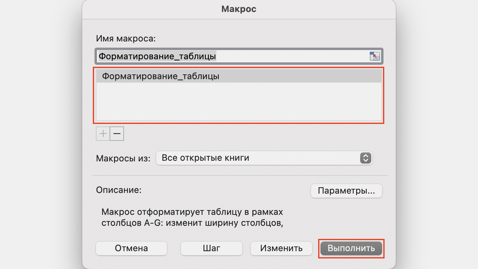
Скриншот: Skillbox Media
Готово — вторая таблица с помощью макроса форматируется так же, как и первая.
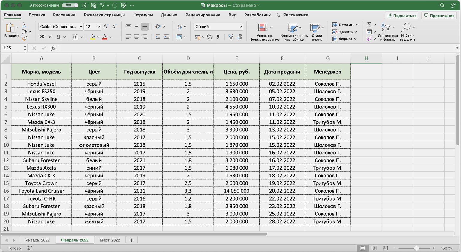
Скриншот: Skillbox Media
То же самое можно сделать и на третьем листе для таблицы продаж за март. Более того, этот же макрос можно будет запустить и в следующем квартале, когда сервис автосалона выгрузит таблицы с новыми данными.

Научитесь: Excel + Google Таблицы с нуля до PRO
Узнать больше
Using Excel Macros can speed up work and save you a lot of time.
One way of getting the VBA code is to record the macro and take the code it generates. However, that code by macro recorder is often full of code that is not really needed. Also macro recorder has some limitations.
So it pays to have a collection of useful VBA macro codes that you can have in your back pocket and use it when needed.
While writing an Excel VBA macro code may take some time initially, once it’s done, you can keep it available as a reference and use it whenever you need it next.
In this massive article, I am going to list some useful Excel macro examples that I need often and keep stashed away in my private vault.
I will keep updating this tutorial with more macro examples. If you think something should be on the list, just leave a comment.
You can bookmark this page for future reference.
Now before I get into the Macro Example and give you the VBA code, let me first show you how to use these example codes.
Using the Code from Excel Macro Examples
Here are the steps you need to follow to use the code from any of the examples:
- Open the Workbook in which you want to use the macro.
- Hold the ALT key and press F11. This opens the VB Editor.
- Right-click on any of the objects in the project explorer.
- Go to Insert –> Module.
- Copy and Paste the code in the Module Code Window.
In case the example says that you need to paste the code in the worksheet code window, double click on the worksheet object and copy paste the code in the code window.
Once you have inserted the code in a workbook, you need to save it with a .XLSM or .XLS extension.
How to Run the Macro
Once you have copied the code in the VB Editor, here are the steps to run the macro:
- Go to the Developer tab.
- Click on Macros.

- In the Macro dialog box, select the macro you want to run.
- Click on Run button.

In case you can’t find the developer tab in the ribbon, read this tutorial to learn how to get it.
Related Tutorial: Different ways to run a macro in Excel.
In case the code is pasted in the worksheet code window, you don’t need to worry about running the code. It will automatically run when the specified action occurs.
Now, let’s get into the useful macro examples that can help you automate work and save time.
Note: You will find many instances of an apostrophe (‘) followed by a line or two. These are comments that are ignored while running the code and are placed as notes for self/reader.
In case you find any error in the article or the code, please be awesome and let me know.

Excel Macro Examples
Below macro examples are covered in this article:
Unhide All Worksheets at One Go
If you are working in a workbook that has multiple hidden sheets, you need to unhide these sheets one by one. This could take some time in case there are many hidden sheets.
Here is the code that will unhide all the worksheets in the workbook.
'This code will unhide all sheets in the workbook
Sub UnhideAllWoksheets()
Dim ws As Worksheet
For Each ws In ActiveWorkbook.Worksheets
ws.Visible = xlSheetVisible
Next ws
End Sub
The above code uses a VBA loop (For Each) to go through each worksheets in the workbook. It then changes the visible property of the worksheet to visible.
Here is a detailed tutorial on how to use various methods to unhide sheets in Excel.
Hide All Worksheets Except the Active Sheet
If you’re working on a report or dashboard and you want to hide all the worksheet except the one that has the report/dashboard, you can use this macro code.
'This macro will hide all the worksheet except the active sheet
Sub HideAllExceptActiveSheet()
Dim ws As Worksheet
For Each ws In ThisWorkbook.Worksheets
If ws.Name <> ActiveSheet.Name Then ws.Visible = xlSheetHidden
Next ws
End Sub
Sort Worksheets Alphabetically Using VBA
If you have a workbook with many worksheets and you want to sort these alphabetically, this macro code can come in really handy. This could be the case if you have sheet names as years or employee names or product names.
'This code will sort the worksheets alphabetically
Sub SortSheetsTabName()
Application.ScreenUpdating = False
Dim ShCount As Integer, i As Integer, j As Integer
ShCount = Sheets.Count
For i = 1 To ShCount - 1
For j = i + 1 To ShCount
If Sheets(j).Name < Sheets(i).Name Then
Sheets(j).Move before:=Sheets(i)
End If
Next j
Next i
Application.ScreenUpdating = True
End Sub
Protect All Worksheets At One Go
If you have a lot of worksheets in a workbook and you want to protect all the sheets, you can use this macro code.
It allows you to specify the password within the code. You will need this password to unprotect the worksheet.
'This code will protect all the sheets at one go
Sub ProtectAllSheets()
Dim ws As Worksheet
Dim password As String
password = "Test123" 'replace Test123 with the password you want
For Each ws In Worksheets
   ws.Protect password:=password
Next ws
End Sub
Unprotect All Worksheets At One Go
If you have some or all of the worksheets protected, you can just use a slight modification of the code used to protect sheets to unprotect it.
'This code will protect all the sheets at one go
Sub ProtectAllSheets()
Dim ws As Worksheet
Dim password As String
password = "Test123" 'replace Test123 with the password you want
For Each ws In Worksheets
ws.Unprotect password:=password
Next ws
End Sub
Note that the password needs to the same that has been used to lock the worksheets. If it’s not, you will see an error.
Unhide All Rows and Columns
This macro code will unhide all the hidden rows and columns.
This could be really helpful if you get a file from someone else and want to be sure there are no hidden rows/columns.
'This code will unhide all the rows and columns in the Worksheet
Sub UnhideRowsColumns()
Columns.EntireColumn.Hidden = False
Rows.EntireRow.Hidden = False
End Sub
Unmerge All Merged Cells
It’s a common practice to merge cells to make it one. While it does the work, when cells are merged you will not be able to sort the data.
In case you are working with a worksheet with merged cells, use the code below to unmerge all the merged cells at one go.
'This code will unmerge all the merged cells
Sub UnmergeAllCells()
ActiveSheet.Cells.UnMerge
End Sub
Note that instead of Merge and Center, I recommend using the Centre Across Selection option.
Save Workbook With TimeStamp in Its Name
A lot of time, you may need to create versions of your work. These are quite helpful in long projects where you work with a file over time.
A good practice is to save the file with timestamps.
Using timestamps will allow you to go back to a certain file to see what changes were made or what data was used.
Here is the code that will automatically save the workbook in the specified folder and add a timestamp whenever it’s saved.
'This code will Save the File With a Timestamp in its name
Sub SaveWorkbookWithTimeStamp()
Dim timestamp As String
timestamp = Format(Date, "dd-mm-yyyy") & "_" & Format(Time, "hh-ss")
ThisWorkbook.SaveAs "C:UsersUsernameDesktopWorkbookName" & timestamp
End Sub
You need to specify the folder location and the file name.
In the above code, “C:UsersUsernameDesktop is the folder location I have used. You need to specify the folder location where you want to save the file. Also, I have used a generic name “WorkbookName” as the filename prefix. You can specify something related to your project or company.
Save Each Worksheet as a Separate PDF
If you work with data for different years or divisions or products, you may have the need to save different worksheets as PDF files.
While it could be a time-consuming process if done manually, VBA can really speed it up.
Here is a VBA code that will save each worksheet as a separate PDF.
'This code will save each worsheet as a separate PDF
Sub SaveWorkshetAsPDF()
Dim ws As Worksheet
For Each ws In Worksheets
ws.ExportAsFixedFormat xlTypePDF, "C:UsersSumitDesktopTest" & ws.Name & ".pdf"
Next ws
End Sub
In the above code, I have specified the address of the folder location in which I want to save the PDFs. Also, each PDF will get the same name as that of the worksheet. You will have to modify this folder location (unless your name is also Sumit and you’re saving it in a test folder on the desktop).
Note that this code works for worksheets only (and not chart sheets).
Save Each Worksheet as a Separate PDF
Here is the code that will save your entire workbook as a PDF in the specified folder.
'This code will save the entire workbook as PDF
Sub SaveWorkshetAsPDF()
ThisWorkbook.ExportAsFixedFormat xlTypePDF, "C:UsersSumitDesktopTest" & ThisWorkbook.Name & ".pdf"
End Sub
You will have to change the folder location to use this code.
Convert All Formulas into Values
Use this code when you have a worksheet that contains a lot of formulas and you want to convert these formulas to values.
'This code will convert all formulas into values
Sub ConvertToValues()
With ActiveSheet.UsedRange
.Value = .Value
End With
End Sub
This code automatically identifies cells are used and convert it into values.
Protect/Lock Cells with Formulas
You may want to lock cells with formulas when you have a lot of calculations and you don’t want to accidentally delete it or change it.
Here is the code that will lock all the cells that have formulas, while all the other cells are not locked.
'This macro code will lock all the cells with formulas
Sub LockCellsWithFormulas()
With ActiveSheet
   .Unprotect
   .Cells.Locked = False
   .Cells.SpecialCells(xlCellTypeFormulas).Locked = True
   .Protect AllowDeletingRows:=True
End With
End Sub
Related Tutorial: How to Lock Cells in Excel.
Protect All Worksheets in the Workbook
Use the below code to protect all the worksheets in a workbook at one go.
'This code will protect all sheets in the workbook
Sub ProtectAllSheets()
Dim ws As Worksheet
For Each ws In Worksheets
ws.Protect
Next ws
End Sub
This code will go through all the worksheets one by one and protect it.
In case you want to unprotect all the worksheets, use ws.Unprotect instead of ws.Protect in the code.
Insert A Row After Every Other Row in the Selection
Use this code when you want to insert a blank row after every row in the selected range.
'This code will insert a row after every row in the selection
Sub InsertAlternateRows()
Dim rng As Range
Dim CountRow As Integer
Dim i As Integer
Set rng = Selection
CountRow = rng.EntireRow.Count
For i = 1 To CountRow
ActiveCell.EntireRow.Insert
ActiveCell.Offset(2, 0).Select
Next i
End Sub
Similarly, you can modify this code to insert a blank column after every column in the selected range.
Automatically Insert Date & Timestamp in the Adjacent Cell
A timestamp is something you use when you want to track activities.
For example, you may want to track activities such as when was a particular expense incurred, what time did the sale invoice was created, when was the data entry done in a cell, when was the report last updated, etc.
Use this code to insert a date and time stamp in the adjacent cell when an entry is made or the existing contents are edited.
'This code will insert a timestamp in the adjacent cell
Private Sub Worksheet_Change(ByVal Target As Range)
On Error GoTo Handler
If Target.Column = 1 And Target.Value <> "" Then
Application.EnableEvents = False
Target.Offset(0, 1) = Format(Now(), "dd-mm-yyyy hh:mm:ss")
Application.EnableEvents = True
End If
Handler:
End Sub
Note that you need to insert this code in the worksheet code window (and not the in module code window as we have done in other Excel macro examples so far). To do this, in the VB Editor, double click on the sheet name on which you want this functionality. Then copy and paste this code in that sheet’s code window.
Also, this code is made to work when the data entry is done in Column A (note that the code has the line Target.Column = 1). You can change this accordingly.
Highlight Alternate Rows in the Selection
Highlighting alternate rows can increase the readability of your data tremendously. This can be useful when you need to take a print out and go through the data.
Here is a code that will instantly highlight alternate rows in the selection.
'This code would highlight alternate rows in the selection
Sub HighlightAlternateRows()
Dim Myrange As Range
Dim Myrow As Range
Set Myrange = Selection
For Each Myrow In Myrange.Rows
   If Myrow.Row Mod 2 = 1 Then
      Myrow.Interior.Color = vbCyan
   End If
Next Myrow
End Sub
Note that I have specified the color as vbCyan in the code. You can specify other colors as well (such as vbRed, vbGreen, vbBlue).
Highlight Cells with Misspelled Words
Excel doesn’t have a spell check as it has in Word or PowerPoint. While you can run the spell check by hitting the F7 key, there is no visual cue when there is a spelling mistake.
Use this code to instantly highlight all the cells that have a spelling mistake in it.
'This code will highlight the cells that have misspelled words
Sub HighlightMisspelledCells()
Dim cl As Range
For Each cl In ActiveSheet.UsedRange
If Not Application.CheckSpelling(word:=cl.Text) Then
cl.Interior.Color = vbRed
End If
Next cl
End Sub
Note that the cells that are highlighted are those that have text that Excel considers as a spelling error. In many cases, it would also highlight names or brand terms that it doesn’t understand.
Refresh All Pivot Tables in the Workbook
If you have more than one Pivot Table in the workbook, you can use this code to refresh all these Pivot tables at once.
'This code will refresh all the Pivot Table in the Workbook
Sub RefreshAllPivotTables()
Dim PT As PivotTable
For Each PT In ActiveSheet.PivotTables
PT.RefreshTable
Next PT
End Sub
You can read more about refreshing Pivot Tables here.
Change the Letter Case of Selected Cells to Upper Case
While Excel has the formulas to change the letter case of the text, it makes you do that in another set of cells.
Use this code to instantly change the letter case of the text in the selected text.
'This code will change the Selection to Upper Case
Sub ChangeCase()
Dim Rng As Range
For Each Rng In Selection.Cells
If Rng.HasFormula = False Then
Rng.Value = UCase(Rng.Value)
End If
Next Rng
End Sub
Note that in this case, I have used UCase to make the text case Upper. You can use LCase for lower case.
Highlight All Cells With Comments
Use the below code to highlight all the cells that have comments in it.
'This code will highlight cells that have comments`
Sub HighlightCellsWithComments()
ActiveSheet.Cells.SpecialCells(xlCellTypeComments).Interior.Color = vbBlue
End Sub
In this case, I have used vbBlue to give a blue color to the cells. You can change this to other colors if you want.
Highlight Blank Cells With VBA
While you can highlight blank cell with conditional formatting or using the Go to Special dialog box, if you have to do it quite often, it’s better to use a macro.
Once created, you can have this macro in the Quick Access Toolbar or save it in your personal macro workbook.
Here is the VBA macro code:
'This code will highlight all the blank cells in the dataset
Sub HighlightBlankCells()
Dim Dataset as Range
Set Dataset = Selection
Dataset.SpecialCells(xlCellTypeBlanks).Interior.Color = vbRed
End Sub
In this code, I have specified the blank cells to be highlighted in the red color. You can choose other colors such as blue, yellow, cyan, etc.
How to Sort Data by Single Column
You can use the below code to sort data by the specified column.
Sub SortDataHeader()
Range("DataRange").Sort Key1:=Range("A1"), Order1:=xlAscending, Header:=xlYes
End Sub
Note that the I have created a named range with the name ‘DataRange’ and have used it instead of the cell references.
Also there are three key parameters that are used here:
- Key1 – This is the on which you want to sort the data set. In the above example code, the data will be sorted based on the values in column A.
- Order- Here you need to specify whether you want to sort the data in ascending or descending order.
- Header – Here you need to specify whether your data has headers or not.
Read more on how to sort data in Excel using VBA.
How to Sort Data by Multiple Columns
Suppose you have a dataset as shown below:

Below is the code that will sort the data based on multiple columns:
Sub SortMultipleColumns()
With ActiveSheet.Sort
 .SortFields.Add Key:=Range("A1"), Order:=xlAscending
 .SortFields.Add Key:=Range("B1"), Order:=xlAscending
 .SetRange Range("A1:C13")
 .Header = xlYes
 .Apply
End With
End Sub
Note that here I have specified to first sort based on column A and then based on column B.
The output would be something as shown below:


How to Get Only the Numeric Part from a String in Excel
If you want to extract only the numeric part or only the text part from a string, you can create a custom function in VBA.
You can then use this VBA function in the worksheet (just like regular Excel functions) and it will extract only the numeric or text part from the string.
Something as shown below:

Below is the VBA code that will create a function to extract numeric part from a string:
'This VBA code will create a function to get the numeric part from a string
Function GetNumeric(CellRef As String)
Dim StringLength As Integer
StringLength = Len(CellRef)
For i = 1 To StringLength
If IsNumeric(Mid(CellRef, i, 1)) Then Result = Result & Mid(CellRef, i, 1)
Next i
GetNumeric = Result
End Function
You need place in code in a module, and then you can use the function =GetNumeric in the worksheet.
This function will take only one argument, which is the cell reference of the cell from which you want to get the numeric part.
Similarly, below is the function that will get you only the text part from a string in Excel:
'This VBA code will create a function to get the text part from a string
Function GetText(CellRef As String)
Dim StringLength As Integer
StringLength = Len(CellRef)
For i = 1 To StringLength
If Not (IsNumeric(Mid(CellRef, i, 1))) Then Result = Result & Mid(CellRef, i, 1)
Next i
GetText = Result
End Function
So these are some of the useful Excel macro codes that you can use in your day-to-day work to automate tasks and be a lot more productive.
Other Excel tutorials you may like:
- How to Delete Macros in Excel
- How to Enable Macros in Excel?