The solver function in excel - Word и Excel - помощь в работе с программами

Solver is a Microsoft Excel add-in program you can use for what-if analysis. Use Solver to find an optimal (maximum or minimum) value for a formula in one cell — called the objective cell — subject to constraints, or limits, on the values of other formula cells on a worksheet. Solver works with a group of cells, called decision variables or simply variable cells that are used in computing the formulas in the objective and constraint cells. Solver adjusts the values in the decision variable cells to satisfy the limits on constraint cells and produce the result you want for the objective cell.

Put simply, you can use Solver to determine the maximum or minimum value of one cell by changing other cells. For example, you can change the amount of your projected advertising budget and see the effect on your projected profit amount.

Note: Versions of Solver prior to Excel 2007 referred to the objective cell as the «target cell,» and the decision variable cells as «changing cells» or «adjustable cells». Many improvements were made to the Solver add-in for Excel 2010, so if you’re using Excel 2007 your experience will be slightly different.

In the following example, the level of advertising in each quarter affects the number of units sold, indirectly determining the amount of sales revenue, the associated expenses, and the profit. Solver can change the quarterly budgets for advertising (decision variable cells B5:C5), up to a total budget constraint of $20,000 (cell F5), until the total profit (objective cell F7) reaches the maximum possible amount. The values in the variable cells are used to calculate the profit for each quarter, so they are related to the formula objective cell F7, =SUM (Q1 Profit:Q2 Profit).

1. Variable cells

2. Constrained cell

3. Objective cell

After Solver runs, the new values are as follows.

On the Data tab, in the Analysis group, click Solver.

Note: If the Solver command or the Analysis group is not available, you need to activate the Solver add-in. See: How to activate the Solver add-in.
In the Set Objective box, enter a cell reference or name for the objective cell. The objective cell must contain a formula.
Do one of the following:
- If you want the value of the objective cell to be as large as possible, click Max.
- If you want the value of the objective cell to be as small as possible, click Min.
- If you want the objective cell to be a certain value, click Value of, and then type the value in the box.
- In the By Changing Variable Cells box, enter a name or reference for each decision variable cell range. Separate the non-adjacent references with commas. The variable cells must be related directly or indirectly to the objective cell. You can specify up to 200 variable cells.
In the Subject to the Constraints box, enter any constraints that you want to apply by doing the following:
1. In the Solver Parameters dialog box, click Add.
2. In the Cell Reference box, enter the cell reference or name of the cell range for which you want to constrain the value.
3. Click the relationship ( <=, =, >=, int, bin, or dif ) that you want between the referenced cell and the constraint.If you click int, integer appears in the Constraint box. If you click bin, binary appears in the Constraint box. If you click dif, alldifferent appears in the Constraint box.
4. If you choose <=, =, or >= for the relationship in the Constraint box, type a number, a cell reference or name, or a formula.
5. Do one of the following:
  - To accept the constraint and add another, click Add.
  - To accept the constraint and return to the Solver Parameters dialog box, click OK.
    Note You can apply the int, bin, and dif relationships only in constraints on decision variable cells.
    
    You can change or delete an existing constraint by doing the following:
6. In the Solver Parameters dialog box, click the constraint that you want to change or delete.
7. Click Change and then make your changes, or click Delete.
Click Solve and do one of the following:
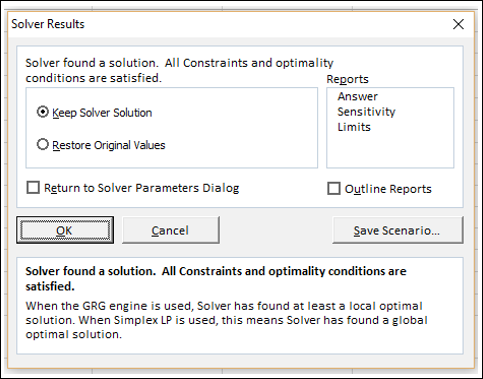
- To keep the solution values on the worksheet, in the Solver Results dialog box, click Keep Solver Solution.
- To restore the original values before you clicked Solve, click Restore Original Values.
- You can interrupt the solution process by pressing Esc. Excel recalculates the worksheet with the last values that are found for the decision variable cells.
- To create a report that is based on your solution after Solver finds a solution, you can click a report type in the Reports box and then click OK. The report is created on a new worksheet in your workbook. If Solver doesn’t find a solution, only certain reports or no reports are available.
- To save your decision variable cell values as a scenario that you can display later, click Save Scenario in the Solver Results dialog box, and then type a name for the scenario in the Scenario Name box.

After you define a problem, click Options in the Solver Parameters dialog box.
In the Options dialog box, select the Show Iteration Results check box to see the values of each trial solution, and then click OK.
In the Solver Parameters dialog box, click Solve.
In the Show Trial Solution dialog box, do one of the following:
- To stop the solution process and display the Solver Results dialog box, click Stop.
- To continue the solution process and display the next trial solution, click Continue.

In the Solver Parameters dialog box, click Options.
Choose or enter values for any of the options on the All Methods, GRG Nonlinear, and Evolutionary tabs in the dialog box.

In the Solver Parameters dialog box, click Load/Save.
Enter a cell range for the model area, and click either Save or Load.

When you save a model, enter the reference for the first cell of a vertical range of empty cells in which you want to place the problem model. When you load a model, enter the reference for the entire range of cells that contains the problem model.

Tip: You can save the last selections in the Solver Parameters dialog box with a worksheet by saving the workbook. Each worksheet in a workbook may have its own Solver selections, and all of them are saved. You can also define more than one problem for a worksheet by clicking Load/Save to save problems individually.

You can choose any of the following three algorithms or solving methods in the Solver Parameters dialog box:

Generalized Reduced Gradient (GRG) Nonlinear Use for problems that are smooth nonlinear.
LP Simplex Use for problems that are linear.
Evolutionary Use for problems that are non-smooth.

Important: You should enable the Solver add-in first. For more information, see Load the Solver add-in.

In the following example, the level of advertising in each quarter affects the number of units sold, indirectly determining the amount of sales revenue, the associated expenses, and the profit. Solver can change the quarterly budgets for advertising (decision variable cells B5:C5), up to a total budget constraint of $20,000 (cell D5), until the total profit (objective cell D7) reaches the maximum possible amount. The values in the variable cells are used to calculate the profit for each quarter, so they are related to the formula objective cell D7, =SUM(Q1 Profit:Q2 Profit).

Variable cells

Constrained cell

Objective cell

After Solver runs, the new values are as follows.

In Excel 2016 for Mac: Click Data > Solver.

In Excel for Mac 2011: Click the Data tab, under Analysis, click Solver.
In Set Objective, enter a cell reference or name for the objective cell.

Note: The objective cell must contain a formula.

Do one of the following:

To	Do this
Make the value of the objective cell as large as possible	Click Max.
Make the value of the objective cell as small as possible	Click Min.
Set the objective cell to a certain value	Click Value Of, and then type the value in the box.

In the By Changing Variable Cells box, enter a name or reference for each decision variable cell range. Separate the nonadjacent references with commas.

The variable cells must be related directly or indirectly to the objective cell. You can specify up to 200 variable cells.

In the Subject to the Constraints box, add any constraints that you want to apply.

To add a constraint, follow these steps:

In the Solver Parameters dialog box, click Add.
In the Cell Reference box, enter the cell reference or name of the cell range for which you want to constrain the value.
On the <= relationship pop-up menu, select the relationship that you want between the referenced cell and the constraint.If you choose <=, =, or >=, in the Constraint box, type a number, a cell reference or name, or a formula.

Note: You can only apply the int, bin, and dif relationships in constraints on decision variable cells.
Do one of the following:

To	Do this
Accept the constraint and add another	Click Add.
Accept the constraint and return to the Solver Parameters dialog box	Click OK.

Click Solve, and then do one of the following:

To	Do this
Keep the solution values on the sheet	Click Keep Solver Solution in the Solver Results dialog box.
Restore the original data	Click Restore Original Values.

Notes:

To interrupt the solution process, press ESC . Excel recalculates the sheet with the last values that are found for the adjustable cells.
To create a report that is based on your solution after Solver finds a solution, you can click a report type in the Reports box and then click OK. The report is created on a new sheet in your workbook. If Solver doesn’t find a solution, the option to create a report is unavailable.
To save your adjusting cell values as a scenario that you can display later, click Save Scenario in the Solver Results dialog box, and then type a name for the scenario in the Scenario Name box.

In Excel 2016 for Mac: Click Data > Solver.

In Excel for Mac 2011: Click the Data tab, under Analysis, click Solver.
After you define a problem, in the Solver Parameters dialog box, click Options.
Select the Show Iteration Results check box to see the values of each trial solution, and then click OK.
In the Solver Parameters dialog box, click Solve.

In the Show Trial Solution dialog box, do one of the following:

To	Do this
Stop the solution process and display the Solver Results dialog box	Click Stop.
Continue the solution process and display the next trial solution	Click Continue.

In Excel 2016 for Mac: Click Data > Solver.

In Excel for Mac 2011: Click the Data tab, under Analysis, click Solver.

Click Options, and then in the Options or Solver Options dialog box, choose one or more of the following options:

To	Do this
Set solution time and iterations	On the All Methods tab, under Solving Limits, in the Max Time (Seconds) box, type the number of seconds that you want to allow for the solution time. Then, in the Iterations box, type the maximum number of iterations that you want to allow. Note: If the solution process reaches the maximum time or number of iterations before Solver finds a solution, Solver displays the Show Trial Solution dialog box.
Set the degree of precision	On the All Methods tab, in the Constraint Precision box, type the degree of precision that you want. The smaller the number, the higher the precision.
Set the degree of convergence	On the GRG Nonlinear or Evolutionary tab, in the Convergence box, type the amount of relative change that you want to allow in the last five iterations before Solver stops with a solution. The smaller the number, the less relative change is allowed.

Do this

Set solution time and iterations

On the All Methods tab, under Solving Limits, in the Max Time (Seconds) box, type the number of seconds that you want to allow for the solution time. Then, in the Iterations box, type the maximum number of iterations that you want to allow.

Note: If the solution process reaches the maximum time or number of iterations before Solver finds a solution, Solver displays the Show Trial Solution dialog box.

Set the degree of precision

On the All Methods tab, in the Constraint Precision box, type the degree of precision that you want. The smaller the number, the higher the precision.

Set the degree of convergence

On the GRG Nonlinear or Evolutionary tab, in the Convergence box, type the amount of relative change that you want to allow in the last five iterations before Solver stops with a solution. The smaller the number, the less relative change is allowed.

Click OK.
In the Solver Parameters dialog box, click Solve or Close.

In Excel 2016 for Mac: Click Data > Solver.

In Excel for Mac 2011: Click the Data tab, under Analysis, click Solver.
Click Load/Save, enter a cell range for the model area, and then click either Save or Load.

When you save a model, enter the reference for the first cell of a vertical range of empty cells in which you want to place the problem model. When you load a model, enter the reference for the entire range of cells that contains the problem model.

Tip: You can save the last selections in the Solver Parameters dialog box with a sheet by saving the workbook. Each sheet in a workbook may have its own Solver selections, and all of them are saved. You can also define more than one problem for a sheet by clicking Load/Save to save problems individually.

In Excel 2016 for Mac: Click Data > Solver.

In Excel for Mac 2011: Click the Data tab, under Analysis, click Solver.
On the Select a Solving Method pop-up menu, select one of the following:

Solving Method	Description
GRG (Generalized Reduced Gradient) Nonlinear	The default choice, for models using most Excel functions other than IF, CHOOSE, LOOKUP and other “step” functions.
Simplex LP	Use this method for linear programming problems. Your model should use SUM, SUMPRODUCT, + — and * in formulas that depend on the variable cells.
Evolutionary	This method, based on genetic algorithms, is best when your model uses IF, CHOOSE, or LOOKUP with arguments that depend on the variable cells.

Because add-in programs aren’t supported in Excel for the web, you won’t be able to use the Solver add-in to run what-if analysis on your data to help you find optimal solutions.

If you have the Excel desktop application, you can use the Open in Excel button to open your workbook to use the Solver add-in.

More help on using Solver

For more detailed help on Solver contact:

Frontline Systems, Inc.
P.O. Box 4288
Incline Village, NV 89450-4288
(775) 831-0300
Web site: http://www.solver.com
E-mail: info@solver.com
Solver Help at www.solver.com.

Need more help?

You can always ask an expert in the Excel Tech Community or get support in the Answers community.

Как включить Солвер в Excel

Как мы уже упоминали, Solver включен в Excel как сторонняя надстройка, но сначала вам нужно включить его, чтобы использовать.

Для этого откройте Excel и нажмите Файл> Параметры открыть меню параметров Excel.

Открытие меню параметров в Excel

в Параметры Excel окно, нажмите Надстройки вкладка для просмотра настроек для надстроек Excel.

Вкладка надстроек Excel

в Надстройки На вкладке вы увидите список доступных надстроек Excel.

Выбрать Надстройки Excel от управлять раскрывающееся меню внизу окна, затем нажмите Идти кнопка.

Управление надстройками Excel

в Надстройки установите флажок рядом с Надстройка Солвера вариант, затем нажмите Хорошо подтвердить.

Включение Excel Solver добавить в

Как только вы нажмете Хорошо, надстройка Solver будет включена, и вы сможете начать ее использовать.

Использование Солвера в Microsoft Excel

Надстройка Solver будет доступна для использования, как только она будет включена. Для начала вам понадобится электронная таблица Excel с соответствующими данными, чтобы вы могли использовать Солвер. Чтобы показать вам, как использовать Солвер, мы будем использовать пример математической задачи.

Исходя из нашего предыдущего предложения, существует электронная таблица, показывающая стоимость дорогостоящего оборудования. Чтобы заплатить за это оборудование, бизнес должен продать определенное количество продуктов, чтобы заплатить за оборудование.

Для этого запроса несколько переменных могут измениться для достижения цели. Вы можете использовать Solver для определения стоимости продукта для оплаты оборудования на основе заданного количества продуктов.

В качестве альтернативы, если вы установили цену, вы могли бы определить количество продаж, которое вам нужно было бы достичь безубыточности — это проблема, которую мы попытаемся решить с помощью Солвера.

Запуск Солвера в Excel

Чтобы использовать Solver для решения этого типа запроса, нажмите Данные вкладка на панели ленты Excel.

Вкладка «Данные» на ленточной панели Excel

в анализировать раздел нажмите решающее устройство вариант.

Кнопка Солвер в Excel

Это загрузит Параметры решателя окно. Отсюда вы можете настроить запрос Солвера.

Выбор параметров решателя

Во-первых, вам нужно выбрать Установить цель клетка. Для этого сценария мы хотим, чтобы доход в ячейке B6 соответствовал стоимости оборудования в ячейке B1, чтобы достичь безубыточности. Исходя из этого, мы можем определить количество продаж, которое нам нужно сделать.

Ячейка Задать цель в Солвере для Excel

к цифра позволяет найти минимум (Min) или максимум (Максимум) возможное значение для достижения цели, или вы можете установить ручную цифру в Значение коробка.

Лучшим вариантом для нашего тестового запроса будет Min вариант. Это потому, что мы хотим найти минимальное количество продаж, чтобы достичь нашей цели безубыточности. Если вы хотите добиться большего, чем это (например, чтобы получить прибыль), вы можете установить целевой показатель дохода в Значение коробка вместо.

Цена остается неизменной, поэтому количество продаж в ячейке B5 является переменная ячейка, Это значение, которое необходимо увеличить.

Вам нужно будет выбрать это в Изменяя переменные ячейки коробка выбора.

Установка переменных Excel Solver

Вы должны будете установить ограничения дальше. Это тесты, которые Solver будет использовать для определения окончательного значения. Если у вас сложные критерии, вы можете установить несколько ограничений для работы Солвера.

Для этого запроса мы ищем номер дохода, который больше или равен первоначальной стоимости оборудования. Чтобы добавить ограничение, нажмите Добавить кнопка.

Добавление ограничения Excel Solver

Использовать Добавить ограничение окно для определения ваших критериев. В этом примере ячейка B6 (показатель целевого дохода) должна быть больше или равна стоимости оборудования в ячейке B1.

После того, как вы выбрали критерии ограничения, нажмите Хорошо или Добавить кнопок.

Добавление ограничения к запросу Excel Solver

Прежде чем вы сможете выполнить свой запрос Solver, вам необходимо подтвердить метод решения, который будет использовать Solver.

По умолчанию это установлено на GRG нелинейный вариант, но есть другие доступные методы решения, Когда вы будете готовы выполнить запрос Солвера, нажмите Решать кнопка.

Окончательные варианты Excel Solver

Запуск Solver Query

Как только вы нажмете РешатьExcel попытается выполнить ваш запрос Солвера. Появится окно результатов, показывающее, был ли запрос успешным.

В нашем примере Solver обнаружил, что минимальное количество продаж, необходимое для соответствия стоимости оборудования (и, следовательно, безубыточности), составило 4800.

Вы можете выбрать Keep Solver Solution вариант, если вы довольны изменениями, внесенными Солвером, или Восстановить исходные значения если нет

Чтобы вернуться в окно «Параметры решателя» и внести изменения в свой запрос, нажмите Вернуться к диалогу параметров решателя флажок.

Окно результатов Excel Solver

щелчок Хорошо чтобы закрыть окно результатов, чтобы закончить.

Работа с данными Excel

Надстройка Excel Solver берет сложную идею и делает ее возможной для миллионов пользователей Excel. Однако это нишевая функция, и вы можете использовать Excel для более простых расчетов.

Вы можете использовать Excel для расчета процентных изменений или, если вы работаете с большим количеством данных, вы можете делать перекрестные ссылки на ячейки в нескольких листах Excel. Вы даже можете вставить данные Excel в PowerPoint, если вы ищете другие способы использования ваших данных.

Источник

Одной из самых интересных функций в программе Microsoft Excel является Поиск решения. Вместе с тем, следует отметить, что данный инструмент нельзя отнести к самым популярным среди пользователей в данном приложении. А зря. Ведь эта функция, используя исходные данные, путем перебора, находит наиболее оптимальное решение из всех имеющихся. Давайте выясним, как использовать функцию Поиск решения в программе Microsoft Excel.

Включение функции

Можно долго искать на ленте, где находится Поиск решения, но так и не найти данный инструмент. Просто, для активации данной функции, нужно её включить в настройках программы.

Для того, чтобы произвести активацию Поиска решений в программе Microsoft Excel 2010 года, и более поздних версий, переходим во вкладку «Файл». Для версии 2007 года, следует нажать на кнопку Microsoft Office в левом верхнем углу окна. В открывшемся окне, переходим в раздел «Параметры».

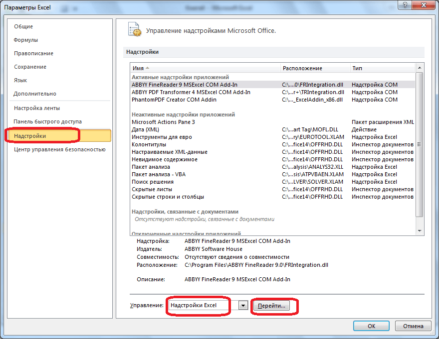
В окне параметров кликаем по пункту «Надстройки». После перехода, в нижней части окна, напротив параметра «Управление» выбираем значение «Надстройки Excel», и кликаем по кнопке «Перейти».

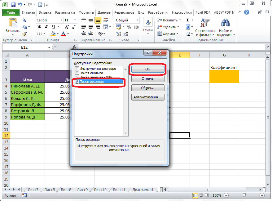
Открывается окно с надстройками. Ставим галочку напротив наименования нужной нам надстройки – «Поиск решения». Жмем на кнопку «OK».

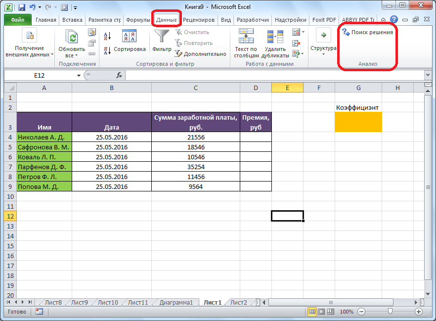
После этого, кнопка для запуска функции Поиска решений появится на ленте Excel во вкладке «Данные».

Подготовка таблицы

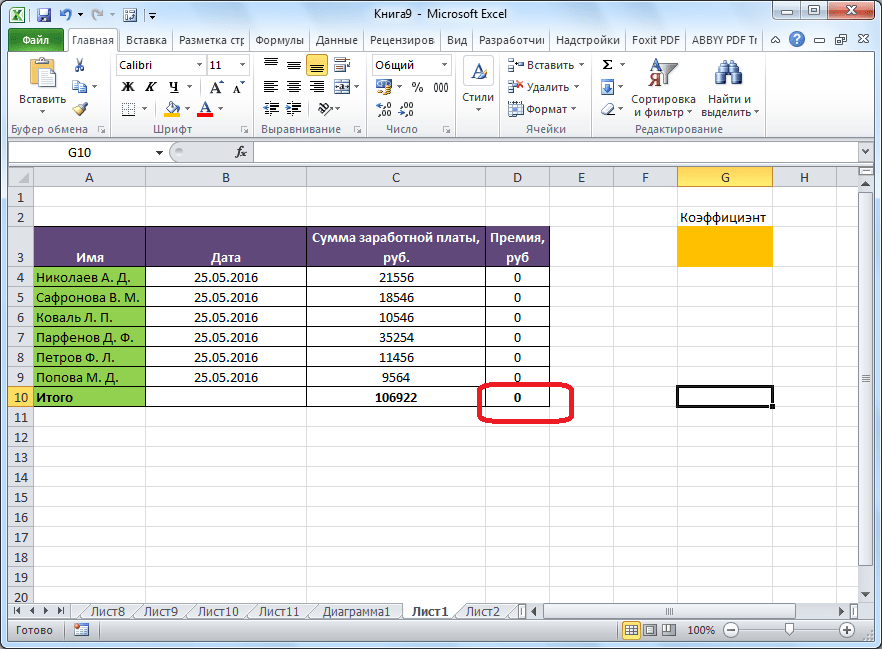
Теперь, после того, как мы активировали функцию, давайте разберемся, как она работает. Легче всего это представить на конкретном примере. Итак, у нас есть таблица заработной платы работников предприятия. Нам следует рассчитать премию каждого работника, которая является произведением заработной платы, указанной в отдельном столбце, на определенный коэффициент. При этом, общая сумма денежных средств, выделяемых на премию, равна 30000 рублей. Ячейка, в которой находится данная сумма, имеет название целевой, так как наша цель подобрать данные именно под это число.

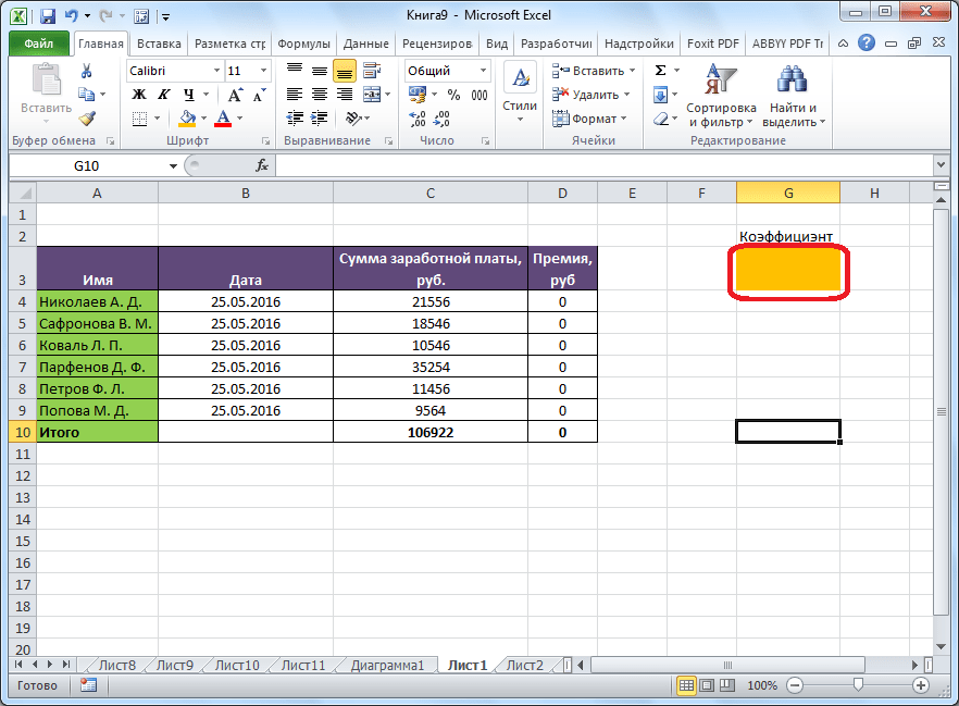
Коэффициент, который применяется для расчета суммы премии, нам предстоит вычислить с помощью функции Поиска решений. Ячейка, в которой он располагается, называется искомой.

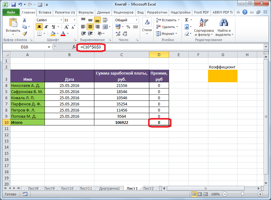
Целевая и искомая ячейка должны быть связанны друг с другом с помощью формулы. В нашем конкретном случае, формула располагается в целевой ячейке, и имеет следующий вид: «=C10*$G$3», где $G$3 – абсолютный адрес искомой ячейки, а «C10» — общая сумма заработной платы, от которой производится расчет премии работникам предприятия.

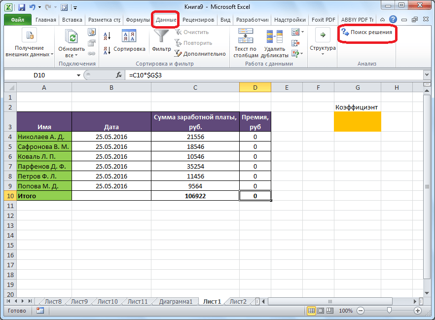
Запуск инструмента Поиск решения

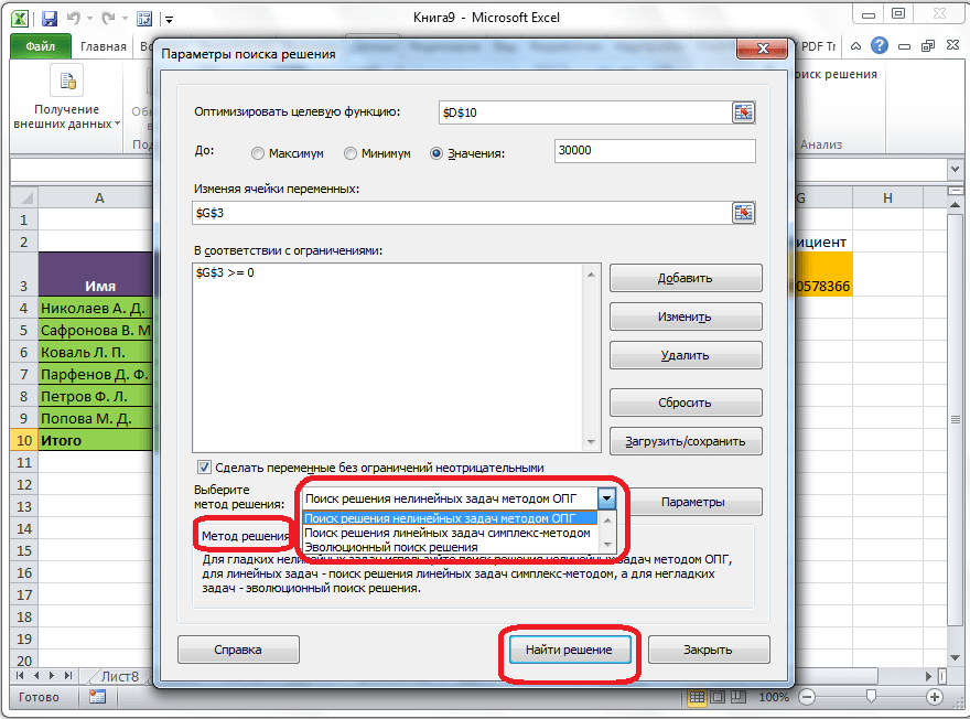
После того, как таблица подготовлена, находясь во вкладке «Данные», жмем на кнопку «Поиск решения», которая расположена на ленте в блоке инструментов «Анализ».

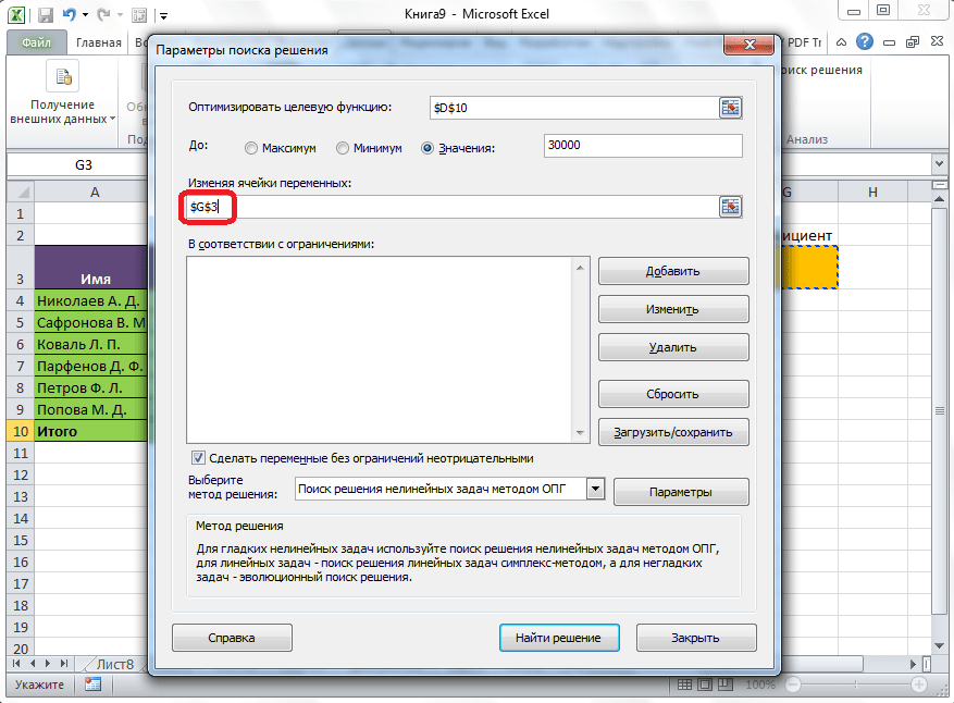
Открывается окно параметров, в которое нужно внести данные. В поле «Оптимизировать целевую функцию» нужно ввести адрес целевой ячейки, где будет располагаться общая сумма премии для всех работников. Это можно сделать либо пропечатав координаты вручную, либо кликнув на кнопку, расположенную слева от поля введения данных.

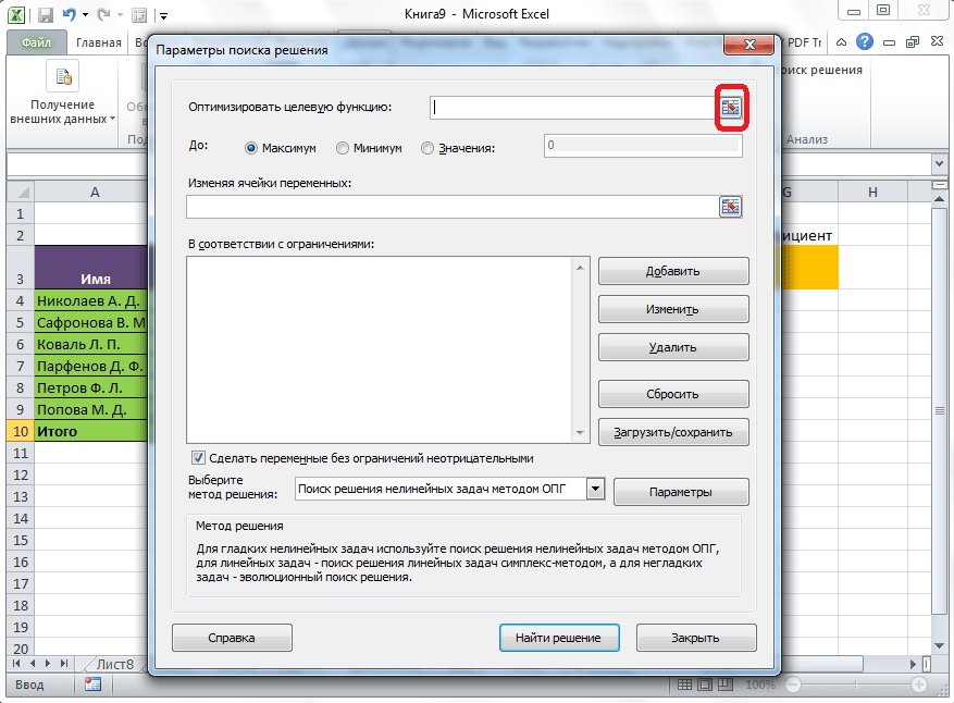
После этого, окно параметров свернется, а вы сможете выделить нужную ячейку таблицы. Затем, требуется опять нажать по той же кнопке слева от формы с введенными данными, чтобы развернуть окно параметров снова.

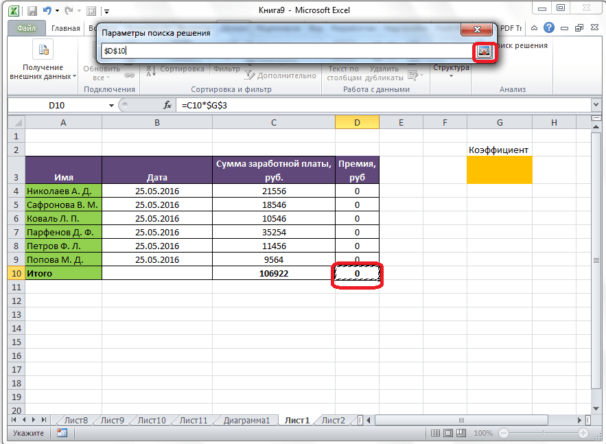
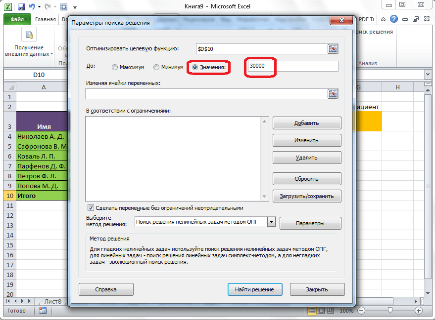
Под окном с адресом целевой ячейки, нужно установить параметры значений, которые будут находиться в ней. Это может быть максимум, минимум, или конкретное значение. В нашем случае, это будет последний вариант. Поэтому, ставим переключатель в позицию «Значения», и в поле слева от него прописываем число 30000. Как мы помним, именно это число по условиям составляет общую сумму премии для всех работников предприятия.

Ниже расположено поле «Изменяя ячейки переменных». Тут нужно указать адрес искомой ячейки, где, как мы помним, находится коэффициент, умножением на который основной заработной платы будет рассчитана величина премии. Адрес можно прописать теми же способами, как мы это делали для целевой ячейки.

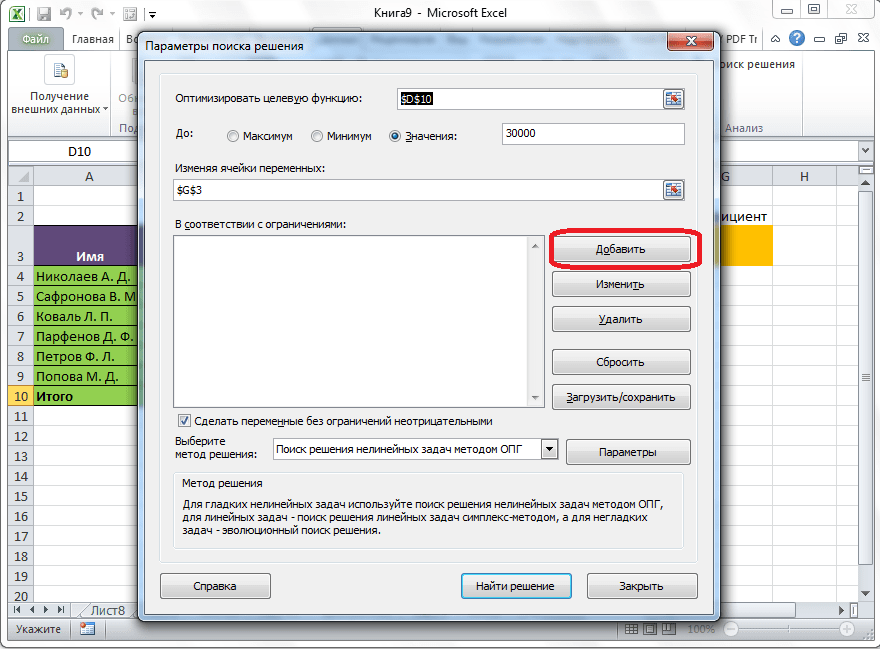
В поле «В соответствии с ограничениями» можно выставить определенные ограничения для данных, например, сделать значения целыми или неотрицательными. Для этого, жмем на кнопку «Добавить».

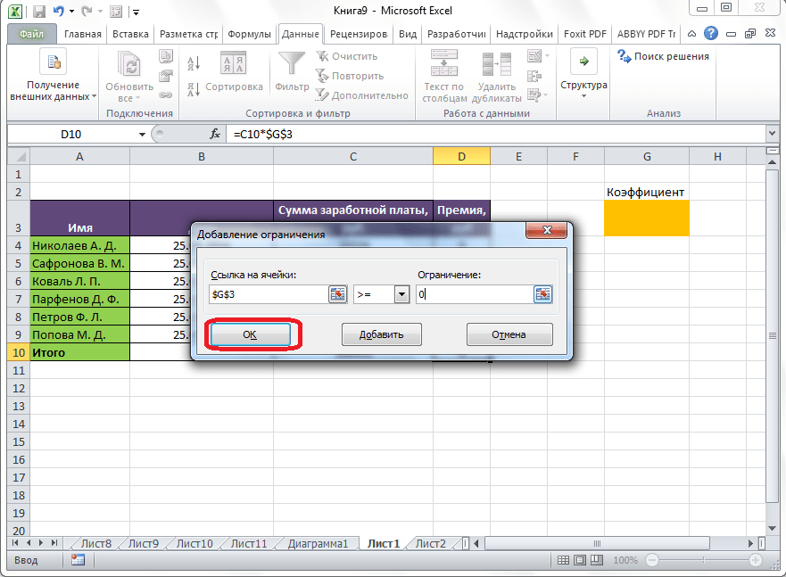
После этого, открывается окно добавления ограничения. В поле «Ссылка на ячейки» прописываем адрес ячеек, относительно которых вводится ограничение. В нашем случае, это искомая ячейка с коэффициентом. Далее проставляем нужный знак: «меньше или равно», «больше или равно», «равно», «целое число», «бинарное», и т.д. В нашем случае, мы выберем знак «больше или равно», чтобы сделать коэффициент положительным числом. Соответственно, в поле «Ограничение» указываем число 0. Если мы хотим настроить ещё одно ограничение, то жмем на кнопку «Добавить». В обратном случае, жмем на кнопку «OK», чтобы сохранить введенные ограничения.

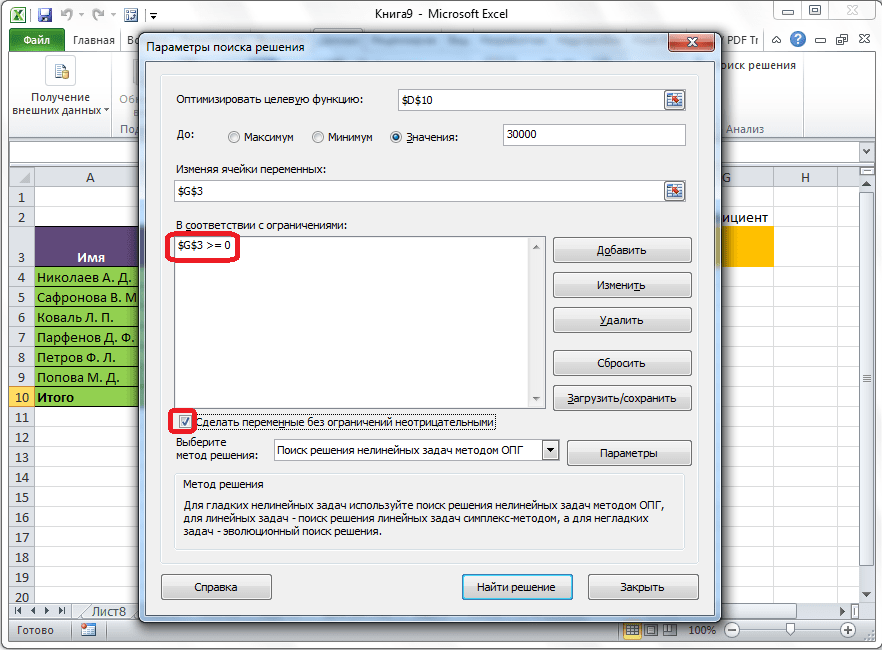
Как видим, после этого, ограничение появляется в соответствующем поле окна параметров поиска решения. Также, сделать переменные неотрицательными, можно установив галочку около соответствующего параметра чуть ниже. Желательно, чтобы установленный тут параметр не противоречил тем, которые вы прописали в ограничениях, иначе, может возникнуть конфликт.

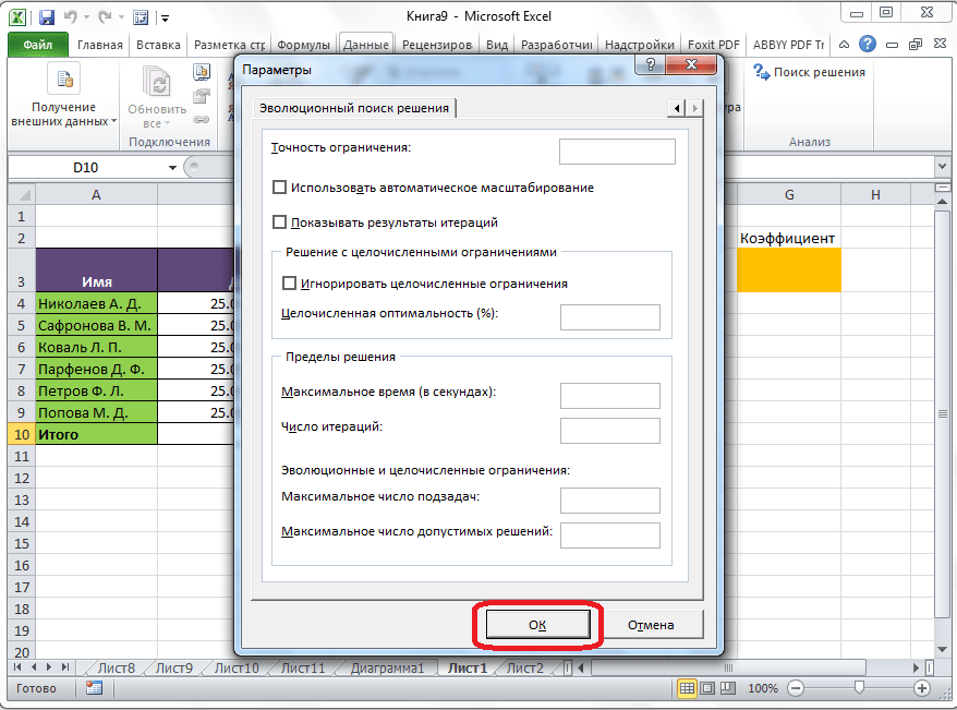
Дополнительные настройки можно задать, кликнув по кнопке «Параметры».

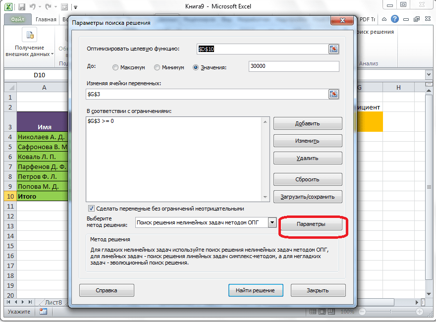
Здесь можно установить точность ограничения и пределы решения. Когда нужные данные введены, жмите на кнопку «OK». Но, для нашего случая, изменять эти параметры не нужно.

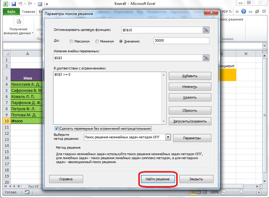
После того, как все настройки установлены, жмем на кнопку «Найти решение».

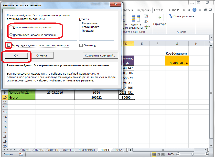
Далее, программа Эксель в ячейках выполняет необходимые расчеты. Одновременно с выдачей результатов, открывается окно, в котором вы можете либо сохранить найденное решение, либо восстановить исходные значения, переставив переключатель в соответствующую позицию. Независимо от выбранного варианта, установив галочку «Вернутся в диалоговое окно параметров», вы можете опять перейти к настройкам поиска решения. После того, как выставлены галочки и переключатели, жмем на кнопку «OK».

Если по какой-либо причине результаты поиска решений вас не удовлетворяют, или при их подсчете программа выдаёт ошибку, то, в таком случае, возвращаемся, описанным выше способом, в диалоговое окно параметров. Пересматриваем все введенные данные, так как возможно где-то была допущена ошибка. В случае, если ошибка найдена не была, то переходим к параметру «Выберите метод решения». Тут предоставляется возможность выбора одного из трех способов расчета: «Поиск решения нелинейных задач методом ОПГ», «Поиск решения линейных задач симплекс-методом», и «Эволюционный поиск решения». По умолчанию, используется первый метод. Пробуем решить поставленную задачу, выбрав любой другой метод. В случае неудачи, повторяем попытку, с использованием последнего метода. Алгоритм действий всё тот же, который мы описывали выше.

Как видим, функция Поиск решения представляет собой довольно интересный инструмент, который, при правильном использовании, может значительно сэкономить время пользователя на различных подсчетах. К сожалению, далеко не каждый пользователь знает о его существовании, не говоря о том, чтобы правильно уметь работать с этой надстройкой. В чем-то данный инструмент напоминает функцию «Подбор параметра…», но в то же время, имеет и существенные различия с ним.

Источник

Solver – это надстройка Microsoft Excel, которую можно использовать для оптимизации в анализе «что, если».

По мнению О’Брайена и Маракаса, оптимизационный анализ является более сложным расширением целенаправленного анализа. Вместо того, чтобы устанавливать конкретное целевое значение для переменной, цель состоит в том, чтобы найти оптимальное значение для одной или нескольких целевых переменных при определенных ограничениях. Затем одна или несколько других переменных меняются неоднократно, с учетом указанных ограничений, пока вы не найдете лучшие значения для целевых переменных.

В Excel вы можете использовать Solver, чтобы найти оптимальное значение (максимальное или минимальное или определенное значение) для формулы в одной ячейке, называемой целевой ячейкой, при условии соблюдения определенных ограничений или ограничений для значений других ячеек формулы на рабочем листе. ,

Это означает, что Солвер работает с группой ячеек, называемых переменными решения, которые используются при вычислении формул в ячейках цели и ограничения. Солвер корректирует значения в ячейках переменных решения, чтобы удовлетворить ограничения на ячейки ограничений и получить желаемый результат для целевой ячейки.

Вы можете использовать Solver, чтобы найти оптимальные решения для различных проблем, таких как –

Определение ежемесячного ассортимента продукции для подразделения по производству лекарств, которое максимизирует прибыльность.
Планирование рабочей силы в организации.
Решение транспортных проблем.
Финансовое планирование и бюджетирование.

Определение ежемесячного ассортимента продукции для подразделения по производству лекарств, которое максимизирует прибыльность.

Планирование рабочей силы в организации.

Решение транспортных проблем.

Финансовое планирование и бюджетирование.

Активация Solver надстройки

Прежде чем приступить к поиску решения проблемы с Solver, убедитесь, что надстройка Solver активирована в Excel следующим образом:

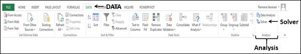
Нажмите вкладку ДАННЫЕ на ленте. Команда Solver должна появиться в группе «Анализ», как показано ниже.

Если вы не можете найти команду Солвера, активируйте ее следующим образом:

Нажмите вкладку ФАЙЛ.
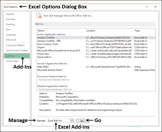
Нажмите Опции на левой панели. Откроется диалоговое окно «Параметры Excel».
Нажмите Надстройки на левой панели.
Выберите Надстройки Excel в поле «Управление» и нажмите «Перейти».

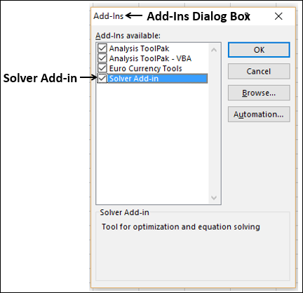
Откроется диалоговое окно «Надстройки». Проверьте Надстройку Solver и нажмите Ok. Теперь вы можете найти команду Solver на ленте под вкладкой DATA.

Методы решения, используемые Solver

Вы можете выбрать один из следующих трех методов решения, которые поддерживает Excel Solver, в зависимости от типа проблемы:

LP Simplex

Используется для линейных задач. Модель Солвера является линейной при следующих условиях:

Целевая ячейка вычисляется путем сложения членов формы (изменяющаяся ячейка) * (постоянная).
Каждое ограничение удовлетворяет требованию линейной модели. Это означает, что каждое ограничение оценивается путем сложения членов формы (изменяющейся ячейки) * (константы) и сравнения сумм с константой.

Целевая ячейка вычисляется путем сложения членов формы (изменяющаяся ячейка) * (постоянная).

Каждое ограничение удовлетворяет требованию линейной модели. Это означает, что каждое ограничение оценивается путем сложения членов формы (изменяющейся ячейки) * (константы) и сравнения сумм с константой.

Обобщенный редуцированный градиент (GRG) нелинейный

Используется для гладких нелинейных задач. Если ваша целевая ячейка, любое из ваших ограничений или оба содержат ссылки на изменяющиеся ячейки, которые не имеют (изменяющейся ячейки) * (постоянной) формы, у вас есть нелинейная модель.

эволюционный

Понимание оценки Солвера

Для Солвера требуются следующие параметры –

Ячейки с переменными решениями
Клетки ограничения
Объективные Клетки
Метод решения

Оценка решателя основана на следующем:

Значения в ячейках переменных решения ограничены значениями в ячейках ограничений.
Вычисление значения в целевой ячейке включает значения в ячейках переменных решения.
Солвер использует выбранный метод решения, чтобы получить оптимальное значение в целевой ячейке.

Значения в ячейках переменных решения ограничены значениями в ячейках ограничений.

Вычисление значения в целевой ячейке включает значения в ячейках переменных решения.

Солвер использует выбранный метод решения, чтобы получить оптимальное значение в целевой ячейке.

Определение проблемы

Предположим, вы анализируете прибыль, полученную компанией, которая производит и продает определенный продукт. Вас просят найти сумму, которая может быть потрачена на рекламу в следующие два квартала, но не более 20 000. Уровень рекламы в каждом квартале влияет на следующее –

Количество проданных единиц, косвенно определяющих сумму выручки от продаж.
Сопутствующие расходы и
Прибыль

Вы можете приступить к определению проблемы как –

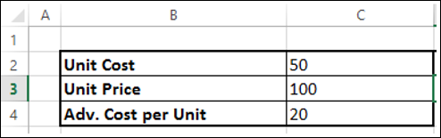
Найти стоимость единицы.
Найти стоимость рекламы на единицу.
Найти цену за единицу.

Затем установите ячейки для необходимых расчетов, как указано ниже.

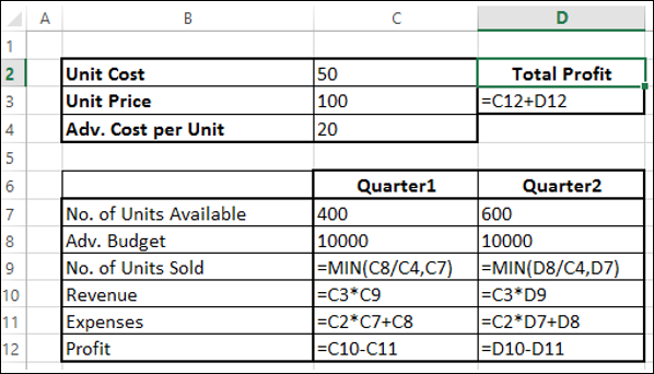
Как вы можете заметить, расчеты сделаны для квартала 1 и квартала 2, которые рассматриваются:

Количество единиц, доступных для продажи в квартале 1, составляет 400, а в квартале 2 – 600 (ячейки – C7 и D7).
Начальные значения для рекламного бюджета установлены как 10000 за квартал (ячейки – C8 и D8).
Количество проданных единиц зависит от стоимости рекламы на единицу и, следовательно, является бюджетом на квартал / Adv. Стоимость за единицу. Обратите внимание, что мы использовали функцию Min, чтобы убедиться, что нет. единиц, проданных в <= нет. из доступных единиц. (Клетки – C9 и D9).
Выручка рассчитывается как цена за единицу * Количество проданных единиц (ячейки – C10 и D10).
Расходы рассчитываются как стоимость единицы * Количество доступных единиц + Adv. Стоимость за этот квартал (Клетки – C11 и D12).
Прибыль – это доход – расходы (ячейки C12 и D12).
Общая прибыль – это прибыль за квартал 1 + прибыль за квартал 2 (ячейка – D3).

Количество единиц, доступных для продажи в квартале 1, составляет 400, а в квартале 2 – 600 (ячейки – C7 и D7).

Начальные значения для рекламного бюджета установлены как 10000 за квартал (ячейки – C8 и D8).

Количество проданных единиц зависит от стоимости рекламы на единицу и, следовательно, является бюджетом на квартал / Adv. Стоимость за единицу. Обратите внимание, что мы использовали функцию Min, чтобы убедиться, что нет. единиц, проданных в <= нет. из доступных единиц. (Клетки – C9 и D9).

Выручка рассчитывается как цена за единицу * Количество проданных единиц (ячейки – C10 и D10).

Расходы рассчитываются как стоимость единицы * Количество доступных единиц + Adv. Стоимость за этот квартал (Клетки – C11 и D12).

Прибыль – это доход – расходы (ячейки C12 и D12).

Общая прибыль – это прибыль за квартал 1 + прибыль за квартал 2 (ячейка – D3).

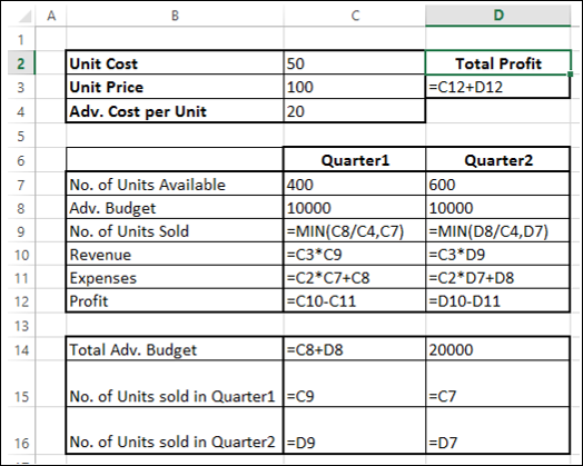
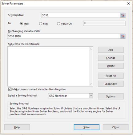
Далее вы можете установить параметры для Солвера, как указано ниже –

Как вы можете заметить, параметры Солвера –

Объективная ячейка – D3, в которой содержится общая прибыль, которую вы хотите максимизировать.
Ячейки с переменными решениями – это C8 и D8, которые содержат бюджеты на два квартала – квартал 1 и квартал 2.
Есть три ячейки ограничения – C14, C15 и C16.
- Ячейка C14, которая содержит общий бюджет, должна установить ограничение 20000 (ячейка D14).
- Ячейка C15, которая содержит номер единиц, проданных в первом квартале, – установить ограничение <= нет. единиц, доступных в Quarter1 (ячейка D15).
- Ячейка C16, которая содержит номер единиц, проданных в Quarter2, это установить ограничение <= нет. единиц, доступных в квартале 2 (ячейка D16).

Объективная ячейка – D3, в которой содержится общая прибыль, которую вы хотите максимизировать.

Ячейки с переменными решениями – это C8 и D8, которые содержат бюджеты на два квартала – квартал 1 и квартал 2.

Есть три ячейки ограничения – C14, C15 и C16.

Ячейка C14, которая содержит общий бюджет, должна установить ограничение 20000 (ячейка D14).

Ячейка C15, которая содержит номер единиц, проданных в первом квартале, – установить ограничение <= нет. единиц, доступных в Quarter1 (ячейка D15).

Ячейка C16, которая содержит номер единиц, проданных в Quarter2, это установить ограничение <= нет. единиц, доступных в квартале 2 (ячейка D16).

Решение проблемы

Следующим шагом является использование Солвера, чтобы найти решение следующим образом:

Шаг 1 – Перейдите в ДАННЫЕ> Анализ> Решатель на ленте. Откроется диалоговое окно «Параметры решателя».

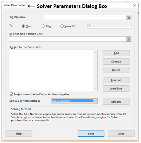
Шаг 2 – В поле «Установить цель» выберите ячейку D3.

Шаг 3 – Выберите Макс.

Шаг 4 – Выберите диапазон C8: D8 в поле « Изменение переменных ячеек» .

Шаг 5 – Затем нажмите кнопку Добавить, чтобы добавить три ограничения, которые вы определили.

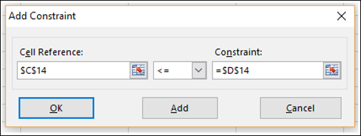
Шаг 6 – Откроется диалоговое окно Add Constraint. Установите ограничение для общего бюджета, как указано ниже, и нажмите «Добавить».

Шаг 7 – Установите ограничение для общего номера. единиц, проданных в квартале 1, как указано ниже, и нажмите кнопку Добавить.

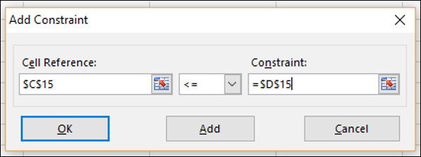
Шаг 8 – Установите ограничение для общего номера. единиц, проданных в квартале 2, как указано ниже, и нажмите кнопку ОК.

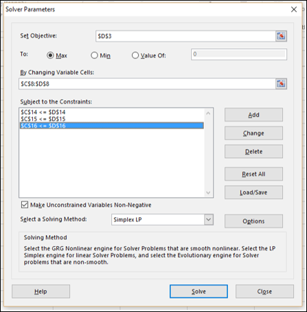
Появится диалоговое окно «Параметры решателя» с тремя ограничениями, добавленными в поле «Подчинить ограничениям».

Шаг 9 – В поле « Выбрать метод решения» выберите Simplex LP.

Шаг 10 – Нажмите кнопку Решить. Откроется диалоговое окно «Результаты решателя». Выберите Keep Solver Solution и нажмите ОК.

Результаты появятся в вашем рабочем листе.

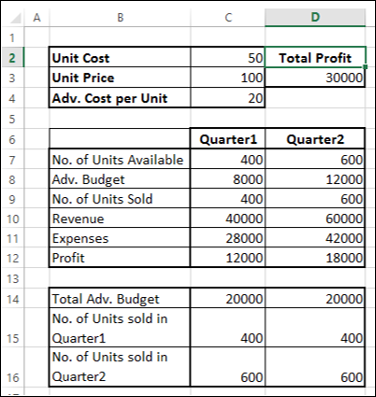
Как вы можете заметить, оптимальное решение, которое дает максимальную общую прибыль с учетом данных ограничений, оказывается следующим:

Общая прибыль – 30000.
Adv. Бюджет на 1 квартал – 8000.
Adv. Бюджет на Квартал2 – 12000.

Пошаговое решение Solver Trial Solutions

Вы можете просмотреть пробные решения Solver, посмотрев результаты итерации.

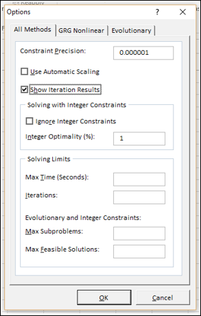
Шаг 1 – Нажмите кнопку «Параметры» в диалоговом окне «Параметры решателя».

Откроется диалоговое окно « Параметры ».

Шаг 2 – Установите флажок «Показать результаты итерации» и нажмите «ОК».

Шаг 3 – Откроется диалоговое окно « Параметры решателя». Нажмите Решить .

Шаг 4 – Появится диалоговое окно « Показать пробное решение », в котором будет отображено сообщение « Солвер остановлен», а текущие значения решения будут отображены на листе .

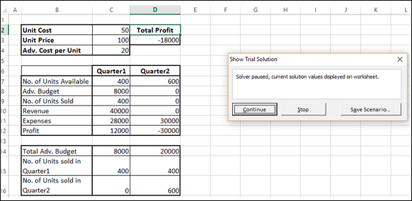
Как вы можете видеть, текущие значения итерации отображаются в ваших рабочих ячейках. Вы можете либо остановить Солвер, принимая текущие результаты, либо продолжить, пока Солвер не найдет решение на следующих шагах.

Шаг 5 – Нажмите Продолжить.

Диалоговое окно « Показать пробное решение » появляется на каждом этапе, и, наконец, после нахождения оптимального решения открывается диалоговое окно «Результаты решения». Ваш рабочий лист обновляется на каждом шаге, и, наконец, отображаются значения результатов.

Сохранение выбора Солвера

У вас есть следующие варианты сохранения для задач, которые вы решаете с помощью Солвера –

Вы можете сохранить последние выбранные значения в диалоговом окне «Параметры решателя» вместе с рабочим листом, сохранив рабочую книгу.

Каждый лист в книге может иметь свои собственные варианты Солвера, и все они будут сохранены при сохранении книги.

Вы также можете определить более одной проблемы на рабочем листе, каждый из которых имеет свой собственный выбор Солвера. В таком случае вы можете загружать и сохранять проблемы по отдельности с помощью диалогового окна «Параметры решателя» «Загрузить / сохранить».

Нажмите кнопку Загрузить / Сохранить . Откроется диалоговое окно загрузки / сохранения.

Чтобы сохранить модель проблемы, введите ссылку для первой ячейки вертикального диапазона пустых ячеек, в который вы хотите поместить модель проблемы. Нажмите Сохранить.

Модель проблемы (набор параметров решателя) появляется начиная с ячейки, которую вы указали в качестве справочной.

Чтобы загрузить модель проблемы, введите ссылку для всего диапазона ячеек, которые содержат модель проблемы. Затем нажмите на кнопку «Загрузить».

Источник

What is Solver in Excel?

The solver in excel is an analysis tool that helps find solutions to complex business problems requiring crucial decisions to be made. For every problem, the goal (objective), variables, and constraints are identified. The solver returns an optimal solution which sets accurate values of the variables, satisfies all constraints, and meets the goal.

For example, the solver helps create the most appropriate project schedule, minimize an organization’s expenses on transportation of its employees, maximize the profits generated by a given marketing plan, and so on.

The solver can solve the following types of problems:

Optimization problems where profits need to be maximized and costs need to be minimized
Arithmetic equations
Linear and nonlinear problems

In optimization problems, the solver in excel helps to minimize or maximize the objective based on certain variables. Being known as a “what-if analysisWhat-If Analysis in Excel is a tool for creating various models, scenarios, and data tables. It enables one to examine how a change in values influences the outcomes in the sheet. The three components of What-If analysis are Scenario Manager, Goal Seek in Excel, and Data Table in Excel.read more” tool, the solver is enabled by the “add-insAn add-in is an extension that adds more features and options to the existing Microsoft Excel.read more” option or the Developer tab of Excel.

What is Solver in Excel?
- The Functioning of the Excel Solver
- How to add “Solver Add-In” in Excel?
- The Terminologies of the Solver in Excel
- The Types of Solving Methods
- How to use the Solver in Excel?
  - Example #1
  - Example #2
- The Applications of the Solver Excel Model
- Frequently Asked Questions
- Recommended Articles

The Functioning of the Excel Solver

For solving a problem, the user has to input certain parameters based on which the solver operates. The tasks of the user followed by the functions of the solver are listed as under:

Identify the goal (objective) of the problem–This tells the solver what has to be done, thereby lending a direction to the solver.
Choose the variables of the problem–This tells the solver the areas it has to work upon. The solver in excel returns the most appropriate values of the variables that meet the goal.
Set the constraints of the problem–This tells the solver to work within the limits defined by the constraints. The solver returns a solution that meets the goal and, at the same time, does not go beyond these limitations.

Hence, the entire solution is focused on the goal of the problem. The solver returns the best possible solution for a problem keeping in mind the set of controls.

How to add “Solver Add-In” in Excel?

The “solver add-in” is not enabled by default in Excel. The two ways to activate the “add-in” are stated as follows:

a. With the “add-ins” option of the File menu

b. With the Developer tabEnabling the developer tab in excel can help the user perform various functions for VBA, Macros and Add-ins like importing and exporting XML, designing forms, etc. This tab is disabled by default on excel; thus, the user needs to enable it first from the options menu.read more

You can download this Solver Excel Template here – Solver Excel Template

a. The steps under “add-ins” option of the File menu are listed as follows:

Click on the File menu.
Select “options” from the various options listed in the menu.
Click on “add-ins.” Select “solver add-in” and click “go.”
Select the checkbox for “solver add-in” and click “Ok.”

b. The steps under the Developer tab option are listed as follows:

In the Developer tab, click on “Excel add-ins” in the “add-ins” group. Select the checkbox “solver add-in” and click “Ok.”

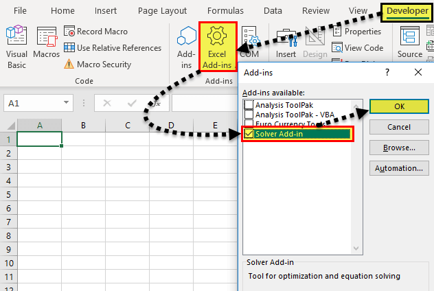
Once installed, the “solver” button appears in the “analysis” group of the Data tab.

The Terminologies of the Solver in Excel

The solver model consists of the objective cells, variable cells, constraints, and formulas that interconnect these components. The excel solver finds an optimal solution to the formula mentioned in the objective cell by changing the variable data cells, given the restrictions of the constraint cells.

Let us understand the terminologies used in the “solver parameters” dialog box. This will be helpful when running the solver. The terms are defined as follows:

Objective cell: This is a single cell which contains a formula. The formula is decision-based and subject to the restrictions of the constraint cells. The value of the objective cell can be minimized, maximized, or set equal to the specified target value.

Decision variable or variable cells: These are the cells in which the solver returns the values based on the objective of the problem. Since these data cells are variable, they can be changed with respect to the objective. In Excel, up to 200 variable cells can be specified.
Constraint cells: These are the limitations within which the given problem is solved. In other words, they are the conditions that should be satisfied.

The Types of Solving Methods

The three methods to solve the data in the excel solver are listed as follows:

GRG nonlinear

The acronym “GRG” stands for “generalized reduced gradient nonlinear.” This method helps solve nonlinear problems. A nonlinear problem may have more than one feasible region. Alternatively, it may have a set of similar values for the variable cells with all the constraints being satisfied.

2. Simplex LP

The acronym “LP” stands for linear problems. This method helps solve linear programming problems and works faster than the GRG nonlinear method. In a linear programming problem, a single objective has to be maximized or minimized subject to certain conditions.

The simplex LP and GRG nonlinear method both are used for smooth problems.

3. Evolutionary

This method helps solve non-smooth problems, which consist of discontinuous functions. The non-smooth problems are the most challenging optimization models to solve.

How to use the Solver in Excel?

Let us consider some examples to understand the solver tool of Excel.

You can download this Solver Excel Template here – Solver Excel Template

Example #1

We want to find the value of X and Y in the following arithmetic equation with the help of the solver tool.

56=2X-5+Y²

Step 1: Formulate the equation on an Excel sheet, as shown in the following image.

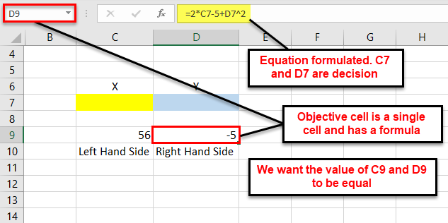
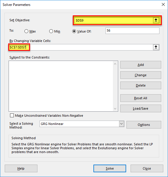
Step 2: Click the “solver” button in the “analysis” group of the Data tab. The “solver parameters” dialog box opens. Enter cell “$D$9” in the objective cell, as shown in the succeeding image. The variable cells are “$C$7:$D$7.”

In the “value of” box, type 56. This is because the right-hand side value of the given equation should be equal to 56.

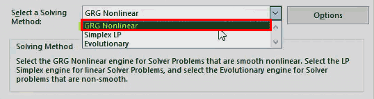
Step 3: Select GRG nonlinear in the “select a solving method” box. Click “solve.”

Note: The GRG nonlinear is the default solving method.

Step 4: The “solver results” box appears. This box may take some time to display depending on the complexity of the model. Select “keep solver solution” and click “Ok,” as shown in the following image.

step13

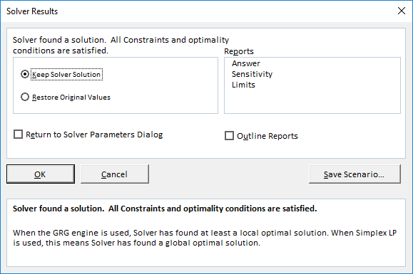
Step 5: The results are shown in the following image. The solver has calculated X as 30.5 and Y as 0. The right-hand and left-hand sides both are equal now.

step14

Example #2

The succeeding image provides the details of an organization that manufactures a television set, stereo, and speaker. The raw materials used are chassis, picture tube, speaker cone, power supply, and electronics. The leftover stock of raw materials is given in G10:G14.

We want to maximize the overall profits given the limited availability of the raw materials.

The variable cells, constraint cells, and the objective cell are highlighted.

step15

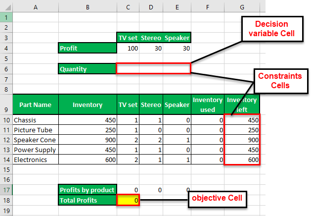
Step 1: Calculate the “used inventory” in F10:F14. The formula is shown in the following image.

step16

Step 2: Click the “solver” button in the “analysis” group of the Data tab. In the “solver parameters” dialog box, click “add” to the right of the “subject to the constraints” box.

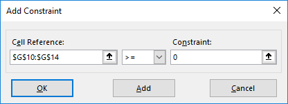
Step 3: The “add constraint” box appears, as shown in the succeeding image. The constraints are defined as follows:

The leftover stock of raw materials should be greater than or equal to zero. So, enter “$G$10:$G$14” in the “cell referenceCell reference in excel is referring the other cells to a cell to use its values or properties. For instance, if we have data in cell A2 and want to use that in cell A1, use =A2 in cell A1, and this will copy the A2 value in A1.read more” box. In the box to the right, type the comparison operator “>=.” In the “constraint” box, enter “0.”
The quantity of the three products (television set, stereo, and speaker) should be greater than or equal to zero. So, enter “$C$6:$E$6>=0” as done for the preceding point.

After entering every constraint, click the “add” button to add it to the “solver parameters” box. Once all constraints have been entered, click “Ok.”

step17

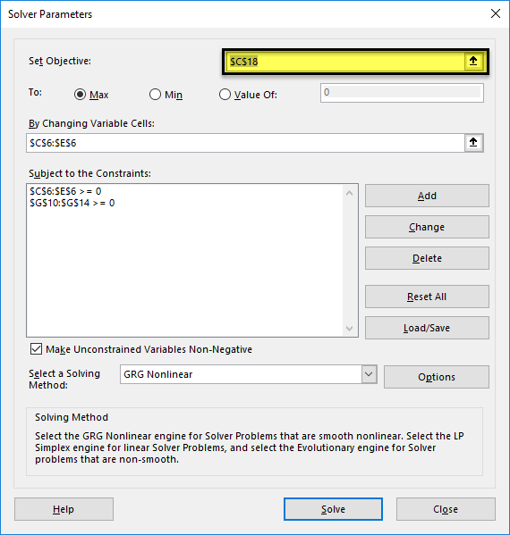
Step 4: In the “solver parameters” box, enter “$C$18” in the “set objective” box. Select the “max” option. In the “by changing variable cells” box, enter “$C$6:$E$6.” Select the solving method as GRG nonlinear. Click “solve.”

step18

Step 5: The output is shown in the following image. The organization must produce 250 television sets, 50 stereos, and 50 speakers to make a profit of $28,000. The product-wise profits are also displayed in C17:E17.

This is an optimal solution given the constraints. With these numbers, the organization will be able to utilize its resources efficiently.

step19

The Applications of the Solver Excel Model

The major applications of the excel solver are listed as follows:

It helps take decisions at the top level of management. For instance, an organization may want to maximize the profits and minimize the costs given the limited resources of inventory and manpower.
It helps solve the day-to-day problems of life which can be converted into arithmetic equations. For instance, a housewife may require an optimal monthly budget to be created which can meet the family’s financial needs, given the limitations.

Frequently Asked Questions

1. Define the solver in Excel.

The solver can solve optimization problems, arithmetic equations, and linear and nonlinear programming models. It helps minimize or maximize the output based on the associated variables and the given constraints.

The solver tool consists of three components which are stated as follows:

• Objective cell – This contains a formula which is to be solved.
• Variable cells – These cells contain variable data which can be adjusted to attain the objective.
• Constraint cells – These are the conditions to be met by the solution of the problem.

The solver solves the problems with the help of three methods GRG nonlinear, simplex LP, and evolutionary. The first two methods are used for smooth problems, while the last helps solve non-smooth problems.

2. What is the purpose of using the solver in Excel?

The objectives of using the solver are listed as follows:

• To find an optimal solution to a problem
• To help minimize or maximize the formula value
• To work on variable data provided the constraints are adhered to
• To perform a comprehensive analysis necessary for making decisions

3. What are the solver parameters in Excel?

The “solver parameters” is a dialog box which appears on clicking the “solver” button in the Data tab. It consists of the following components:

• “Set objective” – This is the objective cell categorized into “max,” “min,” and “value of.” The “max” and “min” help maximize or minimize the formula value respectively. The “value of” category helps set the desired target value.
• “By changing variable cells” – This consists of a range of variable data cells that are changed to achieve the goal.
• “Subject to the constraints” – These are the constraints that can be added, modified, and deleted depending on the requirement.
• “Load/save” button – This saves the current model and displays the stored parameters.
• “Select a solving method” – This consists of the method to solve the problem. Any one of the three methods (GRG nonlinear, simplex LP, and evolutionary) can be selected.
• “Solve” button – This is clicked once all the data has been entered in the tool. It takes the user to the “solver results” dialog box.

Note: If the variable cells are non-adjacent, select the range by pressing and holding the “Ctrl” key.

Load the Solver Add-in

To load the solver add-in, execute the following steps.

1. On the File tab, click Options.

2. Under Add-ins, select Solver Add-in and click on the Go button.

3. Check Solver Add-in and click OK.

4. You can find the Solver on the Data tab, in the Analyze group.

Formulate the Model

The model we are going to solve looks as follows in Excel.

1. To formulate this linear programming model, answer the following three questions.

a. What are the decisions to be made? For this problem, we need Excel to find out how much to order of each product (bicycles, mopeds and child seats).

b. What are the constraints on these decisions? The constrains here are that the amount of capital and storage used by the products cannot exceed the limited amount of capital and storage (resources) available. For example, each bicycle uses 300 units of capital and 0.5 unit of storage.

c. What is the overall measure of performance for these decisions? The overall measure of performance is the total profit of the three products, so the objective is to maximize this quantity.

2. To make the model easier to understand, create the following named ranges.

Range Name	Cells
UnitProfit	C4:E4
OrderSize	C12:E12
ResourcesUsed	G7:G8
ResourcesAvailable	I7:I8
TotalProfit	I12

3. Insert the following three SUMPRODUCT functions.

Explanation: The amount of capital used equals the sumproduct of the range C7:E7 and OrderSize. The amount of storage used equals the sumproduct of the range C8:E8 and OrderSize. Total Profit equals the sumproduct of UnitProfit and OrderSize.

Trial and Error

With this formulation, it becomes easy to analyze any trial solution.

For example, if we order 20 bicycles, 40 mopeds and 100 child seats, the total amount of resources used does not exceed the amount of resources available. This solution has a total profit of 19000.

It is not necessary to use trial and error. We shall describe next how the Excel Solver can be used to quickly find the optimal solution.

Solve the Model

To find the optimal solution, execute the following steps.

1. On the Data tab, in the Analyze group, click Solver.

Enter the solver parameters (read on). The result should be consistent with the picture below.

You have the choice of typing the range names or clicking on the cells in the spreadsheet.

2. Enter TotalProfit for the Objective.

3. Click Max.

4. Enter OrderSize for the Changing Variable Cells.

5. Click Add to enter the following constraint.

6. Check ‘Make Unconstrained Variables Non-Negative’ and select ‘Simplex LP’.

7. Finally, click Solve.

Result:

The optimal solution:

Conclusion: it is optimal to order 94 bicycles and 54 mopeds. This solution gives the maximum profit of 25600. This solution uses all the resources available. Try it yourself. Download the Excel file, enter the solver parameters (previous 7 steps) and find the optimal solution.

Источник

Full Guide to Solver in Excel: How to Use + Install (2023)

We make many assumptions when creating financial models in Microsoft Excel.

These assumptions also have limitations 🚧

If you want to find optimal solutions from a model, you must change these assumptions.

It will take hours to get the answer if you try to change these assumptions manually ⏳

That’s where the Excel Solver feature comes in handy!

In this lesson, I will explain this complex Excel feature in a very easy manner.

You can download the workbook and follow along with me.

What is the Solver add-in?

The Solver add-in is an Excel optimization tool.

You can use the Excel solver to perform a what-if analysis with multiple variables in your model.

It will find an optimal solution for a formula by changing the related variables.

We can add constraints on how much one variable can vary when we change the others.

The solver is useful for Linear programming problems in business, programming, and engineering.

Because of this, Solver is also known as a “Linear Programming Solver.”

However, you can solve both non-smooth or continuous functions as well as smooth non-linear issues with the Excel Solver.

How to add the Solver add-in

The Solver add-in, like the Analysis ToolPak of Excel, is a Microsoft Excel add-in program.

As a result, it is not immediately available in Excel by default.

We must install it 🤔

Let’s look at how to add the Solver add-in to our Excel workbook.

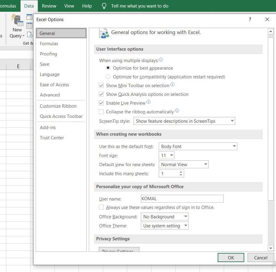
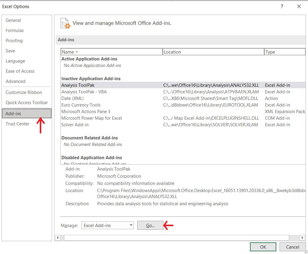
Go to the file tab in your Excel file.

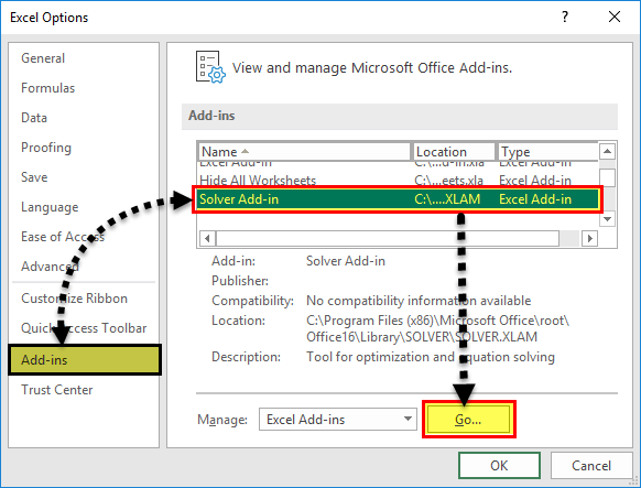
Select options at the bottom of the left-hand sidebar.

Select Add-ins from the Excel options window.

Then in the Manage box, select excel add-ins and click “Go…”.

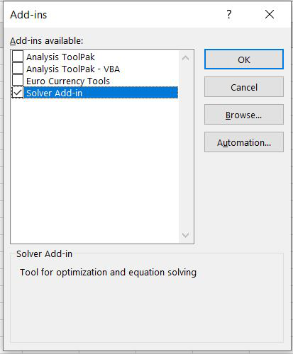
Select the Solver Add-in check box from the Add-ins available box. Then, click OK.

Select the Solver Add-in check box from the Add-ins available box.

Now the Excel Solver Add-ins are loaded to Microsoft excel 👌

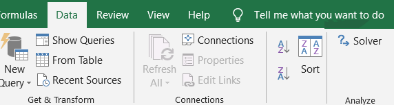
Now, go to the Data tab.

To check view the Excel Solver button - Go to the data tab in the Excel file.

You can see the Excel solver command in the analysis group of the Data tab.

Excel Solver button in the analysis group of the Data tab.

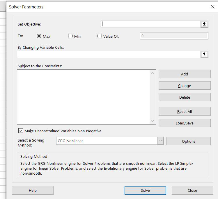
You can click Solver to open the Solver parameters dialog box.

How to use Solver in Excel

It is important to learn different parts of the Solver parameter dialog box before we use it 🧑🏻‍🎓

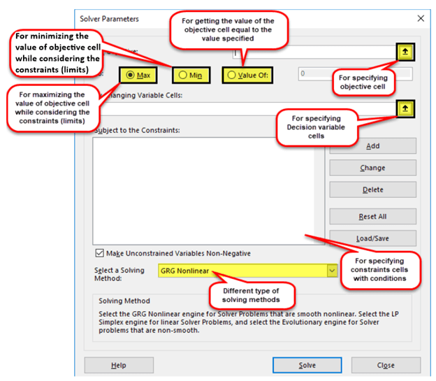
Set Objective

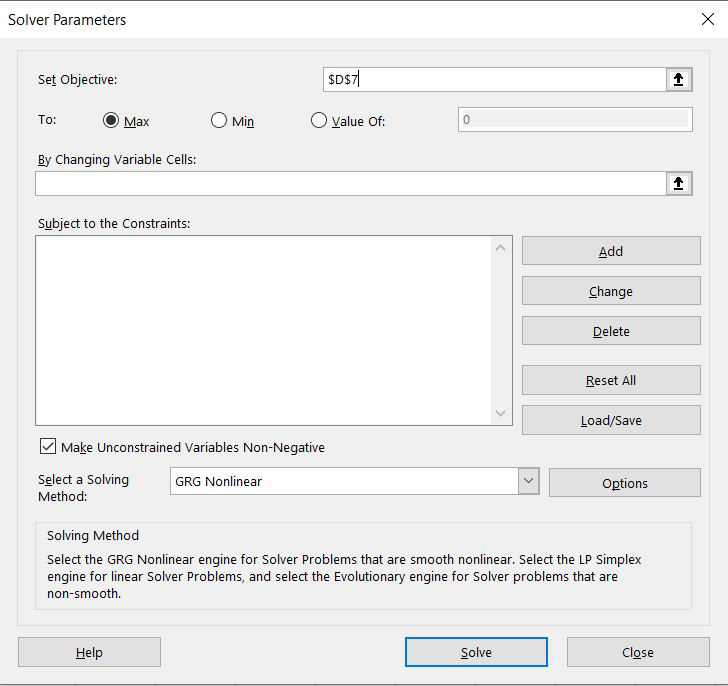
The set objective is the first input for the Excel Solver parameter dialog box.

In the set objective box, we have to select the cell reference for the objective cell.

The objective cell must have a formula.

Kasper Langmann, Microsoft Office Specialist

Then you can set the objective cell to one of the following.

Max
Min
Value of – If you select “Value of”, you must specify the target value in the box.

Solver parameters dialog box - Set objectives

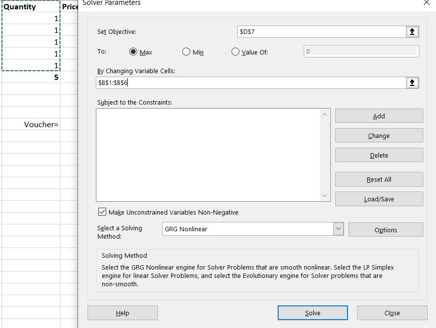
By changing variable cells

In this “by changing variable cells”, you have to select all the variable cells to get the optimal solution.

The variable cells are directly or indirectly related to the target cell.

Currently, you can include up to 200 variable cells for the Excel solver function.

If the variable cells are non-adjacent cells, you have to separate them with commas.

Solver parameters window - By changing variable cells

Subject to the constraints

Excel Solver can find the optimal solution within constraints or limits.

We can add constraints in this constraint box.

Solver parameters window - Subject to constraints

To add constraints, click add button.

Then “Add constraint” box will pop up.

You can select the variable cell for the cell reference box and add the limit in the constraint box.

You must specify the relationship between the cell reference box and the constraint box also.

Do you want to delete or change an existing constraint? 👇🏻

Select that constraint from the Excel Solver parameters dialog box.

Then click the change button to change the existing constraint.

Or click the delete button to delete that.

Kasper Langmann, Microsoft Office Specialist

Select a solving method

In Excel solver, we can select one of the solving methods from the following 3.

GRG non-linear – For solver problems that are smooth nonlinear.
Simplex LP – For linear programming problems.
Evolutionary – For solver problems that are non-smooth.

Excel Solver parameters - Solving methods

Now you are familiar with the Excel solver add-in options window 💪🏻

Let’s use Excel Solver to find a solution for a linear programming model.

Linear programming with Solver add-in

In the below example, we have to find how many units we have to sell in order to get the desired outcome of profit.

Let’s learn step by step how to use the Excel Solver solution to our linear programming problem.

Go to the data tab and click solver to open the Excel Solver.
Select the objective cell reference.

Our goal is to set the total profit in cell B7 to $900.

So, B7 is the objective cell.

As we need to match the value of the objective cell to $900, we have to select the option of “Value of”.

Then type 900, next to the “value of” option.

Excel Solver - Setting objective cell reference to value of $900

Select the variable cells.

The variable for the target value is the quantity for each cell.

So, in this case, the variable cells are B2, C2, and D2.

Excel Solver - Selecting variable cells.

Click the “Add” tab to add constraints for each variable.

Choose each product’s quantity cell as a cell reference.

Then choose the referenced cell’s maximum amount as the constraint.

Next, choose the link between the referred cell.

Here we select “less than or equal sign” because the constraint is maximum quantity.

Again, we need the quantities as whole numbers.

So, we set another constraint for each variable cell as an Integer.

Excel Solver - Adding maximum amounts as constraints

Excel Solver - Set the quantity as an integer.

After entering all constraints, the solver displays all constraints for the particular solution.

Solver displays all constraints for possible solutions

Select the “Simplex LP” as we are solving a linear solver problem and click the “Solve” button at the bottom of the window.

Excel Solver - Selecting the solving method

Then, you can see the Solver results dialog box with options to “keep solver solution” and to “restore original values”.

Select the “keep solver solution” and click “OK”.

To get a total profit of $900, we have to sell 149 in vanilla flavour, 114 in chocolate flavour, and 75 in banana flavour.

That’s it – Now what?

Now you have learned Excel Solver a hidden gem of an Excel 💎

You can use this to solve many problems in financial models.

But, before you use Excel Solver for your model, you must make sure all your functions such as IF, SUMIF, and VLOOKUP are correctly applied in the model.

Otherwise, the Solver will take hours to get the solution and may give incorrect results.

Click here to access my free 30-minute online course where you can learn about IF, SUMIF, and VLOOKUP if you haven’t already.

Frequently asked questions

When you need to change only one input to get the desired outcome of a formula, you can easily use Excel’s inbuilt feature Goal Seek.

We have to specify the formula cell, the target value for the formula cell, and the cell to change in order to get the target value.

Only 200 decision variables are currently supported by Excel solver.

This restriction applies to both linear and nonlinear models.

Another problem is that we cannot ensure that we will obtain the solver model’s optimal solution if it is not linear.

Kasper Langmann2023-01-10T18:48:32+00:00

Page load link

Источник

A solver is a mathematical tool present in MS-Excel that is used to perform calculations by working under some constraints/conditions and then calculates the solution for the problem. It works on the objective cell by changing the variable cells any by using sum constraints.

Solver is present in MS- Excel but for using it we need to activate it. For activating the solver tool we need to do the following steps:

Step 1: Go to File and select options. The following dialog box will appear.

Step 2: Now select the Add-ins option and click on Go and finally click on OK.

Step 3: After clicking OK, Select Solver Add-in and press OK. Now solver will be activated in Excel.

Step 4: Now solver will appear in data section like this.

Now let’s understand how to use solver with the help of an example.

Example:

We went to a mall and we also have a gift voucher worth rs.10,000 and We want to purchase items in such a manner that all the money of the gift voucher gets utilized.

So, suppose we purchased the following items.

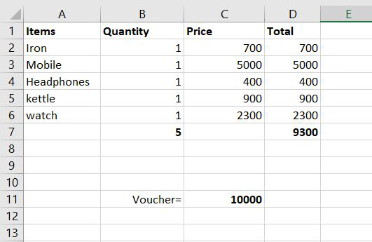
Suppose we purchased the above items in only one quantity and the total came out to be 9300 but the voucher was for rs.10,000. So now we want to use Solver for this purpose. Now let’s see how it will be done.

Step 1: Firstly go on data and find solver there and click it. The following dialog box will appear. Now in this, we have to select the objective in which we want to change our value.

Step 2: In the set objective we have to select the total of the D column because want the value to change from 9300 to 10,000. After clicking on D7 following thing will be displayed on the set objective block.

Step 3: Now in the ‘By changing Variable cell’ we will select the Quantity cell because we want to change the quantity in such a way so that the total amount comes to 10,000.

Step 4: Now we have to set some conditions under which we want our work to get done. So for setting some conditions /constraints, we will click on Add.

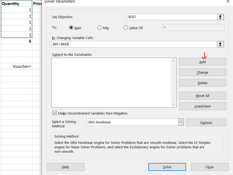
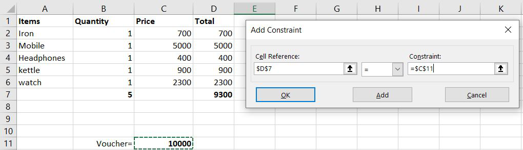
Step 5– Now, a dialog box will appear and we will add 3 conditions. The first condition is that the total amount should be equal to the voucher amount. So we will select cell D7 in a cell reference and then = sign, and finally, we will select cell C11. Now the first condition is added. To add the next condition press Add.

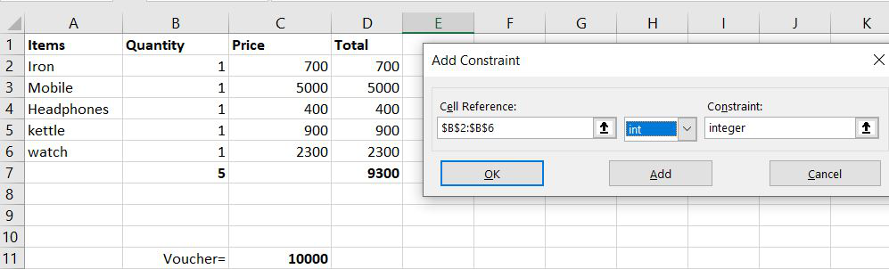
Step 6: For the second condition we will select the Quantity cell because we want the quantity to be an integer value, a whole value. So in cell reference, we will select from B2 to B6 then int, and then again will press Add.

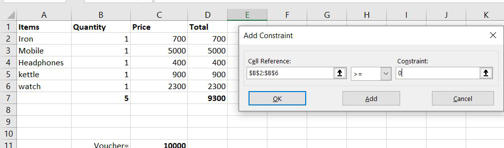
Step 7- Now for the third condition, we want that our item quantity should never be un negative which is not possible in real life. So we will select cells from B2 to B6 and should be >= to zero. Then click Add and cancel.

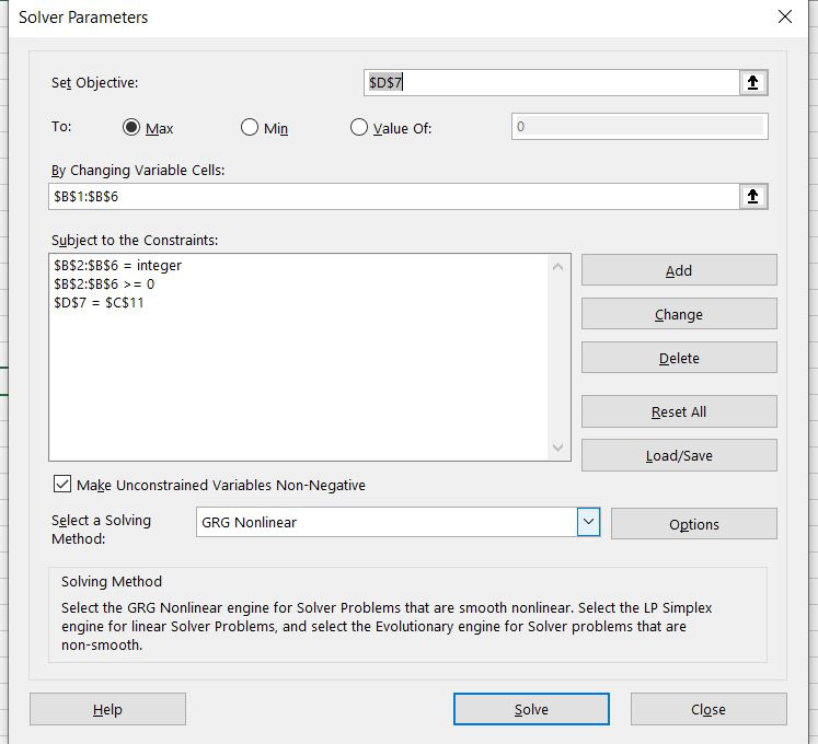
Step 8: Now the following dialog box will show all the 3 conditions that we used and now click on Solve.

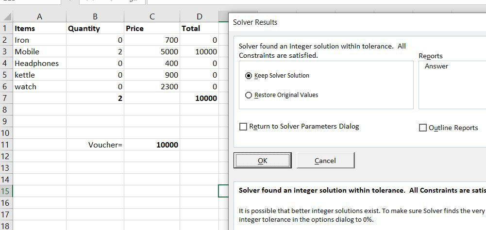
Step 9: By clicking Solve the solver will provide the desired output and to keep the answer we will click on keep solver solution.

So, this is what a solver is, How it is activated by not by default present in Excel and this is how it is used.

Источник

Download Article

Enabling Solver

Analyzing and Solving

Video

Tips

Warnings

This wikiHow teaches you how to use Microsoft Excel’s Solver tool, which allows you to alter different variables in a spreadsheet in order to achieve a desired solution. You can use Solver in both Windows and Mac versions of Excel, though you’ll have to enable Solver before you can begin using it.

1
Open Excel. Click or double-click the Excel app icon, which resembles a green box with a white «X» on it.
- Solver comes pre-installed with both Windows and Mac versions of Excel, but you’ll have to enable it manually.
2
Click Blank workbook. This will open the Excel window, from which point you can proceed with enabling Solver.
- If you have an existing Excel file you’d like to use Solver with, you can open it instead of creating a new file.
Advertisement
3
Click File. It’s a tab in the upper-left side of the Excel window.
- On a Mac, click Tools instead, then skip the next step.
4

Click Options. You’ll find this option at the bottom of the File menu. Doing so brings up the Options window.^[1]
5
Click Add-ins. It’s a tab in the lower-left side of the Options window.
- On a Mac, click Excel Add-ins in the Tools menu.
6
Open the «Add-ins Available» window. Make sure that the «Manage» text box has «Excel Add-ins» listed in it, then click Go at the bottom of the page.
- On a Mac, this window will open after clicking Excel Add-ins in the Tools menu.
7

Install the Solver add-in. Check the «Solver» box in the middle of the page, then click OK. Solver should now appear as a tool in the Data tab that’s at the top of Excel.

1

Understand Solver’s use. Solver can analyze your spreadsheet’s data and any constraints you’ve added to show you possible solutions. This is useful if you’re working with multiple variables.
2
Add your data to your spreadsheet. In order to use Solver, your spreadsheet must have data with different variables and a solution.
- For example, you might create a spreadsheet documenting your various expenses over the course of a month with the output cell resulting in your money left over.
- You can’t use solver on a spreadsheet which doesn’t have solvable data (i.e., your data has to have equations).
3

Click the Data tab. It’s at the top of the Excel window. This will open the Data toolbar.
4

Click Solver. You’ll find this option in the far-right side of the Data toolbar. Doing so opens the Solver window.
5
Select your target cell. Click the cell in which you want to display your Solver solution. This will add it to the «Set Objective» box.
- For example, if you’re creating a budget where the end goal is your monthly income, you would click the final «Income» cell.
6
Set a goal. Check the «Value Of» box, then type your target value into the text box next to «Value Of».
- For example, if your goal is to have $200 at the end of the month, you would type 200 into the text box.
- You can also check either the «Max» or «Min» box in order to prompt Solver to determine the absolute maximum or minimum value.
- Once you’ve set a goal, Solver will attempt to meet that goal by adjusting other variables in your spreadsheet.
7
Add constraints. Constraints set restrictions on the values that Solver can use, which prevents Solver from accidentally nullifying one or more of your spreadsheet’s values. You can add a constraint by doing the following:^[2]
- Click Add
- Click the cell (or select the cells) for which the constraint applies.
- Select a type of constraint from the middle drop-down menu.
- Enter the constraint’s number (e.g., a maximum or minimum).
- Click OK
8

Run Solver. Once you’ve added all of your constraints, click Solve at the bottom of the Solver window. This will prompt Solver to find the optimal solution for your problem.
9

Review the results. When Solver alerts you that it has an answer, you can see the answer by looking at your spreadsheet to see which values were changed.
10
Change your Solver criteria. If the output that you received isn’t ideal for your spreadsheet, click Cancel in the pop-up window, then adjust your objective and constraints.
- If you do like your Solver’s results, you can apply them to your spreadsheet by checking the «Keep Solver Solution» box and then clicking OK.

Ask a Question

200 characters left

Include your email address to get a message when this question is answered.

Submit

Video

Solver is best used for problems such as scheduling employees, determining the lowest price for which you can sell items while meeting a financial goal, and budgeting.

Thanks for submitting a tip for review!

Solver cannot be used in spreadsheets in which there is no «output» or actual solution. For example, you can’t apply solver to a spreadsheet which has no equations.

About This Article

Article SummaryX

1. Enable Solver in the «Add-ins» section of your Excel preferences if necessary.
2. Open a spreadsheet with data you want to analyze.
3. Click Data, then click Solver.
4. Select a cell to use from the «Set Objective» field.
5. Check the «Value Of» box, then enter a desired value.
6. Click Solve.

Did this summary help you?

Thanks to all authors for creating a page that has been read 590,232 times.

Is this article up to date?

Источник

More help on using Solver

Need more help?

See Also

Как включить Солвер в Excel

Использование Солвера в Microsoft Excel

Запуск Солвера в Excel

Выбор параметров решателя

Запуск Solver Query

Работа с данными Excel

Включение функции

Подготовка таблицы

Запуск инструмента Поиск решения

Активация Solver надстройки

Методы решения, используемые Solver

LP Simplex

Обобщенный редуцированный градиент (GRG) нелинейный

эволюционный

Понимание оценки Солвера

Определение проблемы

Решение проблемы

Пошаговое решение Solver Trial Solutions

Сохранение выбора Солвера

What is Solver in Excel?

Table of contents

The Functioning of the Excel Solver

How to add “Solver Add-In” in Excel?

The Terminologies of the Solver in Excel

The Types of Solving Methods

How to use the Solver in Excel?

Example #1

Example #2

The Applications of the Solver Excel Model

Frequently Asked Questions

Recommended Articles

Load the Solver Add-in

Formulate the Model

Trial and Error

Solve the Model

Full Guide to Solver in Excel: How to Use + Install (2023)

What is the Solver add-in?

How to add the Solver add-in

How to use Solver in Excel

Set Objective

By changing variable cells

Subject to the constraints

Select a solving method

Linear programming with Solver add-in

That’s it – Now what?

Frequently asked questions

Video

About This Article

Is this article up to date?