
На чтение 18 мин. Просмотров 75.1k.

сэр Артур Конан Дойл
Это большая ошибка — теоретизировать, прежде чем кто-то получит данные
Эта статья охватывает все, что вам нужно знать об использовании ячеек и диапазонов в VBA. Вы можете прочитать его от начала до конца, так как он сложен в логическом порядке. Или использовать оглавление ниже, чтобы перейти к разделу по вашему выбору.
Рассматриваемые темы включают свойство смещения, чтение
значений между ячейками, чтение значений в массивы и форматирование ячеек.
Содержание
- Краткое руководство по диапазонам и клеткам
- Введение
- Важное замечание
- Свойство Range
- Свойство Cells рабочего листа
- Использование Cells и Range вместе
- Свойство Offset диапазона
- Использование диапазона CurrentRegion
- Использование Rows и Columns в качестве Ranges
- Использование Range вместо Worksheet
- Чтение значений из одной ячейки в другую
- Использование метода Range.Resize
- Чтение Value в переменные
- Как копировать и вставлять ячейки
- Чтение диапазона ячеек в массив
- Пройти через все клетки в диапазоне
- Форматирование ячеек
- Основные моменты
Краткое руководство по диапазонам и клеткам
| Функция | Принимает | Возвращает | Пример | Вид |
| Range | адреса ячеек |
диапазон ячеек |
.Range(«A1:A4») | $A$1:$A$4 |
| Cells | строка, столбец |
одна ячейка |
.Cells(1,5) | $E$1 |
| Offset | строка, столбец |
диапазон | .Range(«A1:A2») .Offset(1,2) |
$C$2:$C$3 |
| Rows | строка (-и) | одна или несколько строк |
.Rows(4) .Rows(«2:4») |
$4:$4 $2:$4 |
| Columns | столбец (-цы) |
один или несколько столбцов |
.Columns(4) .Columns(«B:D») |
$D:$D $B:$D |
Введение
Это третья статья, посвященная трем основным элементам VBA. Этими тремя элементами являются Workbooks, Worksheets и Ranges/Cells. Cells, безусловно, самая важная часть Excel. Почти все, что вы делаете в Excel, начинается и заканчивается ячейками.
Вы делаете три основных вещи с помощью ячеек:
- Читаете из ячейки.
- Пишите в ячейку.
- Изменяете формат ячейки.
В Excel есть несколько методов для доступа к ячейкам, таких как Range, Cells и Offset. Можно запутаться, так как эти функции делают похожие операции.
В этой статье я расскажу о каждом из них, объясню, почему они вам нужны, и когда вам следует их использовать.
Давайте начнем с самого простого метода доступа к ячейкам — с помощью свойства Range рабочего листа.
Важное замечание
Я недавно обновил эту статью, сейчас использую Value2.
Вам может быть интересно, в чем разница между Value, Value2 и значением по умолчанию:
' Value2
Range("A1").Value2 = 56

' Value
Range("A1").Value = 56

' По умолчанию используется значение
Range("A1") = 56
Использование Value может усечь число, если ячейка отформатирована, как валюта. Если вы не используете какое-либо свойство, по умолчанию используется Value.
Лучше использовать Value2, поскольку он всегда будет возвращать фактическое значение ячейки.
Свойство Range
Рабочий лист имеет свойство Range, которое можно использовать для доступа к ячейкам в VBA. Свойство Range принимает тот же аргумент, что и большинство функций Excel Worksheet, например: «А1», «А3: С6» и т.д.
В следующем примере показано, как поместить значение в ячейку с помощью свойства Range.
Sub ZapisVYacheiku()

    ' Запишите число в ячейку A1 на листе 1 этой книги
    ThisWorkbook.Worksheets("Лист1").Range("A1").Value2 = 67

    ' Напишите текст в ячейку A2 на листе 1 этой рабочей книги
    ThisWorkbook.Worksheets("Лист1").Range("A2").Value2 = "Иван Петров"

    ' Запишите дату в ячейку A3 на листе 1 этой книги
    ThisWorkbook.Worksheets("Лист1").Range("A3").Value2 = #11/21/2019#

End Sub
Как видно из кода, Range является членом Worksheets, которая, в свою очередь, является членом Workbook. Иерархия такая же, как и в Excel, поэтому должно быть легко понять. Чтобы сделать что-то с Range, вы должны сначала указать рабочую книгу и рабочий лист, которому она принадлежит.
В оставшейся части этой статьи я буду использовать кодовое имя для ссылки на лист.

Следующий код показывает приведенный выше пример с использованием кодового имени рабочего листа, т.е. Лист1 вместо ThisWorkbook.Worksheets («Лист1»).
Sub IspKodImya ()

    ' Запишите число в ячейку A1 на листе 1 этой книги
     Sheet1.Range("A1").Value2 = 67

    ' Напишите текст в ячейку A2 на листе 1 этой рабочей книги
    Sheet1.Range("A2").Value2 = "Иван Петров"

    ' Запишите дату в ячейку A3 на листе 1 этой книги
    Sheet1.Range("A3").Value2 = #11/21/2019#

End Sub
Вы также можете писать в несколько ячеек, используя свойство
Range
Sub ZapisNeskol()

    ' Запишите число в диапазон ячеек
    Sheet1.Range("A1:A10").Value2 = 67

    ' Написать текст в несколько диапазонов ячеек
    Sheet1.Range("B2:B5,B7:B9").Value2 = "Иван Петров"

End Sub
Свойство Cells рабочего листа
У Объекта листа есть другое свойство, называемое Cells, которое очень похоже на Range . Есть два отличия:
- Cells возвращают диапазон только одной ячейки.
- Cells принимает строку и столбец в качестве аргументов.
В приведенном ниже примере показано, как записывать значения
в ячейки, используя свойства Range и Cells.
Sub IspCells()

    ' Написать в А1
    Sheet1.Range("A1").Value2 = 10
    Sheet1.Cells(1, 1).Value2  = 10

    ' Написать в А10
    Sheet1.Range("A10").Value2 = 10
    Sheet1.Cells(10, 1).Value2  = 10

    ' Написать в E1
    Sheet1.Range("E1").Value2 = 10
    Sheet1.Cells(1, 5).Value2  = 10

End Sub
Вам должно быть интересно, когда использовать Cells, а когда Range. Использование Range полезно для доступа к одним и тем же ячейкам при каждом запуске макроса.
Например, если вы использовали макрос для вычисления суммы и
каждый раз записывали ее в ячейку A10, тогда Range подойдет для этой задачи.
Использование свойства Cells полезно, если вы обращаетесь к
ячейке по номеру, который может отличаться. Проще объяснить это на примере.
В следующем коде мы просим пользователя указать номер столбца. Использование Cells дает нам возможность использовать переменное число для столбца.
Sub ZapisVPervuyuPustuyuYacheiku()

    Dim UserCol As Integer

    ' Получить номер столбца от пользователя
    UserCol = Application.InputBox("Пожалуйста, введите номер столбца...", Type:=1)

    ' Написать текст в выбранный пользователем столбец
    Sheet1.Cells(1, UserCol).Value2 = "Иван Петров"

End Sub
В приведенном выше примере мы используем номер для столбца,
а не букву.
Чтобы использовать Range здесь, потребуется преобразовать эти значения в ссылку на
буквенно-цифровую ячейку, например, «С1». Использование свойства Cells позволяет нам
предоставить строку и номер столбца для доступа к ячейке.
Иногда вам может понадобиться вернуть более одной ячейки, используя номера строк и столбцов. В следующем разделе показано, как это сделать.
Использование Cells и Range вместе
Как вы уже видели, вы можете получить доступ только к одной ячейке, используя свойство Cells. Если вы хотите вернуть диапазон ячеек, вы можете использовать Cells с Range следующим образом:
Sub IspCellsSRange()

    With Sheet1
        ' Запишите 5 в диапазон A1: A10, используя свойство Cells
        .Range(.Cells(1, 1), .Cells(10, 1)).Value2 = 5

        ' Диапазон B1: Z1 будет выделен жирным шрифтом
        .Range(.Cells(1, 2), .Cells(1, 26)).Font.Bold = True

    End With

End Sub
Как видите, вы предоставляете начальную и конечную ячейку
диапазона. Иногда бывает сложно увидеть, с каким диапазоном вы имеете дело,
когда значением являются все числа. Range имеет свойство Address, которое
отображает буквенно-цифровую ячейку для любого диапазона. Это может
пригодиться, когда вы впервые отлаживаете или пишете код.
В следующем примере мы распечатываем адрес используемых нами
диапазонов.
Sub PokazatAdresDiapazona()

    ' Примечание. Использование подчеркивания позволяет разделить строки кода.
    With Sheet1

        ' Запишите 5 в диапазон A1: A10, используя свойство Cells
        .Range(.Cells(1, 1), .Cells(10, 1)).Value2 = 5
        Debug.Print "Первый адрес: " _
            + .Range(.Cells(1, 1), .Cells(10, 1)).Address

        ' Диапазон B1: Z1 будет выделен жирным шрифтом
        .Range(.Cells(1, 2), .Cells(1, 26)).Font.Bold = True
        Debug.Print "Второй адрес : " _
            + .Range(.Cells(1, 2), .Cells(1, 26)).Address

    End With

End Sub
В примере я использовал Debug.Print для печати в Immediate Window. Для просмотра этого окна выберите «View» -> «в Immediate Window» (Ctrl + G).


Свойство Offset диапазона
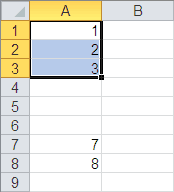
У диапазона есть свойство, которое называется Offset. Термин «Offset» относится к отсчету от исходной позиции. Он часто используется в определенных областях программирования. С помощью свойства «Offset» вы можете получить диапазон ячеек того же размера и на определенном расстоянии от текущего диапазона. Это полезно, потому что иногда вы можете выбрать диапазон на основе определенного условия. Например, на скриншоте ниже есть столбец для каждого дня недели. Учитывая номер дня (т.е. понедельник = 1, вторник = 2 и т.д.). Нам нужно записать значение в правильный столбец.

Сначала мы попытаемся сделать это без использования Offset.
' Это Sub тесты с разными значениями
Sub TestSelect()

    ' Понедельник
    SetValueSelect 1, 111.21
    ' Среда
    SetValueSelect 3, 456.99
    ' Пятница
    SetValueSelect 5, 432.25
    ' Воскресение
    SetValueSelect 7, 710.17

End Sub

' Записывает значение в столбец на основе дня
Public Sub SetValueSelect(lDay As Long, lValue As Currency)

    Select Case lDay
        Case 1: Sheet1.Range("H3").Value2 = lValue
        Case 2: Sheet1.Range("I3").Value2 = lValue
        Case 3: Sheet1.Range("J3").Value2 = lValue
        Case 4: Sheet1.Range("K3").Value2 = lValue
        Case 5: Sheet1.Range("L3").Value2 = lValue
        Case 6: Sheet1.Range("M3").Value2 = lValue
        Case 7: Sheet1.Range("N3").Value2 = lValue
    End Select

End Sub
Как видно из примера, нам нужно добавить строку для каждого возможного варианта. Это не идеальная ситуация. Использование свойства Offset обеспечивает более чистое решение.
' Это Sub тесты с разными значениями
Sub TestOffset()

    DayOffSet 1, 111.01
    DayOffSet 3, 456.99
    DayOffSet 5, 432.25
    DayOffSet 7, 710.17

End Sub

Public Sub DayOffSet(lDay As Long, lValue As Currency)

    ' Мы используем значение дня с Offset, чтобы указать правильный столбец
    Sheet1.Range("G3").Offset(, lDay).Value2 = lValue

End Sub
Как видите, это решение намного лучше. Если количество дней увеличилось, нам больше не нужно добавлять код. Чтобы Offset был полезен, должна быть какая-то связь между позициями ячеек. Если столбцы Day в приведенном выше примере были случайными, мы не могли бы использовать Offset. Мы должны были бы использовать первое решение.
Следует иметь в виду, что Offset сохраняет размер диапазона. Итак .Range («A1:A3»).Offset (1,1) возвращает диапазон B2:B4. Ниже приведены еще несколько примеров использования Offset.
Sub IspOffset()

    ' Запись в В2 - без Offset
    Sheet1.Range("B2").Offset().Value2 = "Ячейка B2"

    ' Написать в C2 - 1 столбец справа
    Sheet1.Range("B2").Offset(, 1).Value2 = "Ячейка C2"

    ' Написать в B3 - 1 строка вниз
    Sheet1.Range("B2").Offset(1).Value2 = "Ячейка B3"

    ' Запись в C3 - 1 столбец справа и 1 строка вниз
    Sheet1.Range("B2").Offset(1, 1).Value2 = "Ячейка C3"

    ' Написать в A1 - 1 столбец слева и 1 строка вверх
    Sheet1.Range("B2").Offset(-1, -1).Value2 = "Ячейка A1"

    ' Запись в диапазон E3: G13 - 1 столбец справа и 1 строка вниз
    Sheet1.Range("D2:F12").Offset(1, 1).Value2 = "Ячейки E3:G13"

End Sub
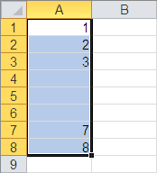
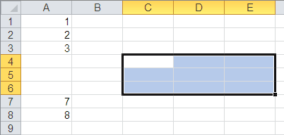
Использование диапазона CurrentRegion
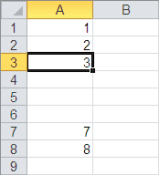
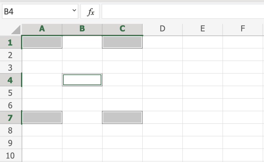
CurrentRegion возвращает диапазон всех соседних ячеек в данный диапазон. На скриншоте ниже вы можете увидеть два CurrentRegion. Я добавил границы, чтобы прояснить CurrentRegion.

Строка или столбец пустых ячеек означает конец CurrentRegion.
Вы можете вручную проверить
CurrentRegion в Excel, выбрав диапазон и нажав Ctrl + Shift + *.
Если мы возьмем любой диапазон
ячеек в пределах границы и применим CurrentRegion, мы вернем диапазон ячеек во
всей области.
Например:
Range («B3»). CurrentRegion вернет диапазон B3:D14
Range («D14»). CurrentRegion вернет диапазон B3:D14
Range («C8:C9»). CurrentRegion вернет диапазон B3:D14 и так далее
Как пользоваться
Мы получаем CurrentRegion следующим образом
' CurrentRegion вернет B3:D14 из приведенного выше примера
Dim rg As Range
Set rg = Sheet1.Range("B3").CurrentRegion
Только чтение строк данных
Прочитать диапазон из второй строки, т.е. пропустить строку заголовка.
' CurrentRegion вернет B3:D14 из приведенного выше примера
Dim rg As Range
Set rg = Sheet1.Range("B3").CurrentRegion

' Начало в строке 2 - строка после заголовка
Dim i As Long
For i = 2 To rg.Rows.Count
    ' текущая строка, столбец 1 диапазона
    Debug.Print rg.Cells(i, 1).Value2
Next i
Удалить заголовок
Удалить строку заголовка (т.е. первую строку) из диапазона. Например, если диапазон — A1:D4, это возвратит A2:D4
' CurrentRegion вернет B3:D14 из приведенного выше примера
Dim rg As Range
Set rg = Sheet1.Range("B3").CurrentRegion

' Удалить заголовок
Set rg = rg.Resize(rg.Rows.Count - 1).Offset(1)

' Начните со строки 1, так как нет строки заголовка
Dim i As Long
For i = 1 To rg.Rows.Count
    ' текущая строка, столбец 1 диапазона
    Debug.Print rg.Cells(i, 1).Value2
Next i
Использование Rows и Columns в качестве Ranges
Если вы хотите что-то сделать со всей строкой или столбцом,
вы можете использовать свойство «Rows и
Columns» на рабочем листе. Они оба принимают один параметр — номер строки
или столбца, к которому вы хотите получить доступ.
Sub IspRowIColumns()

    ' Установите размер шрифта столбца B на 9
    Sheet1.Columns(2).Font.Size = 9

    ' Установите ширину столбцов от D до F
    Sheet1.Columns("D:F").ColumnWidth = 4

    ' Установите размер шрифта строки 5 до 18
    Sheet1.Rows(5).Font.Size = 18

End Sub
Использование Range вместо Worksheet
Вы также можете использовать Cella, Rows и Columns, как часть Range, а не как часть Worksheet. У вас может быть особая необходимость в этом, но в противном случае я бы избегал практики. Это делает код более сложным. Простой код — твой друг. Это уменьшает вероятность ошибок.
Код ниже выделит второй столбец диапазона полужирным. Поскольку диапазон имеет только две строки, весь столбец считается B1:B2
Sub IspColumnsVRange()

    ' Это выделит B1 и B2 жирным шрифтом.
    Sheet1.Range("A1:C2").Columns(2).Font.Bold = True

End Sub
Чтение значений из одной ячейки в другую
В большинстве примеров мы записали значения в ячейку. Мы
делаем это, помещая диапазон слева от знака равенства и значение для размещения
в ячейке справа. Для записи данных из одной ячейки в другую мы делаем то же
самое. Диапазон назначения идет слева, а диапазон источника — справа.
В следующем примере показано, как это сделать:
Sub ChitatZnacheniya()

    ' Поместите значение из B1 в A1
    Sheet1.Range("A1").Value2 = Sheet1.Range("B1").Value2

    ' Поместите значение из B3 в лист2 в ячейку A1
    Sheet1.Range("A1").Value2 = Sheet2.Range("B3").Value2

    ' Поместите значение от B1 в ячейки A1 до A5
    Sheet1.Range("A1:A5").Value2 = Sheet1.Range("B1").Value2

    ' Вам необходимо использовать свойство «Value», чтобы прочитать несколько ячеек
    Sheet1.Range("A1:A5").Value2 = Sheet1.Range("B1:B5").Value2

End Sub
Как видно из этого примера, невозможно читать из нескольких ячеек. Если вы хотите сделать это, вы можете использовать функцию копирования Range с параметром Destination.
Sub KopirovatZnacheniya()

    ' Сохранить диапазон копирования в переменной
    Dim rgCopy As Range
    Set rgCopy = Sheet1.Range("B1:B5")

    ' Используйте это для копирования из более чем одной ячейки
    rgCopy.Copy Destination:=Sheet1.Range("A1:A5")

    ' Вы можете вставить в несколько мест назначения
    rgCopy.Copy Destination:=Sheet1.Range("A1:A5,C2:C6")

End Sub
Функция Copy копирует все, включая формат ячеек. Это тот же результат, что и ручное копирование и вставка выделения. Подробнее об этом вы можете узнать в разделе «Копирование и вставка ячеек»
Использование метода Range.Resize
При копировании из одного диапазона в другой с использованием присваивания (т.е. знака равенства) диапазон назначения должен быть того же размера, что и исходный диапазон.
Использование функции Resize позволяет изменить размер
диапазона до заданного количества строк и столбцов.
Например:
Sub ResizePrimeri()

    ' Печатает А1
    Debug.Print Sheet1.Range("A1").Address

    ' Печатает A1:A2
    Debug.Print Sheet1.Range("A1").Resize(2, 1).Address

    ' Печатает A1:A5
    Debug.Print Sheet1.Range("A1").Resize(5, 1).Address

    ' Печатает A1:D1
    Debug.Print Sheet1.Range("A1").Resize(1, 4).Address

    ' Печатает A1:C3
    Debug.Print Sheet1.Range("A1").Resize(3, 3).Address

End Sub
Когда мы хотим изменить наш целевой диапазон, мы можем
просто использовать исходный размер диапазона.
Другими словами, мы используем количество строк и столбцов
исходного диапазона в качестве параметров для изменения размера:
Sub Resize()

    Dim rgSrc As Range, rgDest As Range

    ' Получить все данные в текущей области
    Set rgSrc = Sheet1.Range("A1").CurrentRegion

      ' Получить диапазон назначения
    Set rgDest = Sheet2.Range("A1")
    Set rgDest = rgDest.Resize(rgSrc.Rows.Count, rgSrc.Columns.Count)

    rgDest.Value2 = rgSrc.Value2

End Sub
Мы можем сделать изменение размера в одну строку, если нужно:
Sub Resize2()

    Dim rgSrc As Range

    ' Получить все данные в ткущей области
    Set rgSrc = Sheet1.Range("A1").CurrentRegion

    With rgSrc
        Sheet2.Range("A1").Resize(.Rows.Count, .Columns.Count) = .Value2
    End With

End Sub
Чтение Value в переменные
Мы рассмотрели, как читать из одной клетки в другую. Вы также можете читать из ячейки в переменную. Переменная используется для хранения значений во время работы макроса. Обычно вы делаете это, когда хотите манипулировать данными перед тем, как их записать. Ниже приведен простой пример использования переменной. Как видите, значение элемента справа от равенства записывается в элементе слева от равенства.
Sub IspVar()

    ' Создайте
    Dim val As Integer

    ' Читать число из ячейки
    val = Sheet1.Range("A1").Value2

    ' Добавить 1 к значению
    val = val + 1

    ' Запишите новое значение в ячейку
    Sheet1.Range("A2").Value2 = val

End Sub
Для чтения текста в переменную вы используете переменную
типа String.
Sub IspVarText()

    ' Объявите переменную типа string
    Dim sText As String

    ' Считать значение из ячейки
    sText = Sheet1.Range("A1").Value2

    ' Записать значение в ячейку
    Sheet1.Range("A2").Value2 = sText

End Sub
Вы можете записать переменную в диапазон ячеек. Вы просто
указываете диапазон слева, и значение будет записано во все ячейки диапазона.
Sub VarNeskol()

    ' Считать значение из ячейки
    Sheet1.Range("A1:B10").Value2 = 66

End Sub
Вы не можете читать из нескольких ячеек в переменную. Однако
вы можете читать массив, который представляет собой набор переменных. Мы
рассмотрим это в следующем разделе.
Как копировать и вставлять ячейки
Если вы хотите скопировать и вставить диапазон ячеек, вам не
нужно выбирать их. Это распространенная ошибка, допущенная новыми пользователями
VBA.
Вы можете просто скопировать ряд ячеек, как здесь:
Range("A1:B4").Copy Destination:=Range("C5")
При использовании этого метода копируется все — значения,
форматы, формулы и так далее. Если вы хотите скопировать отдельные элементы, вы
можете использовать свойство PasteSpecial
диапазона.
Работает так:
Range("A1:B4").Copy
Range("F3").PasteSpecial Paste:=xlPasteValues
Range("F3").PasteSpecial Paste:=xlPasteFormats
Range("F3").PasteSpecial Paste:=xlPasteFormulas
В следующей таблице приведен полный список всех типов вставок.
| Виды вставок |
| xlPasteAll |
| xlPasteAllExceptBorders |
| xlPasteAllMergingConditionalFormats |
| xlPasteAllUsingSourceTheme |
| xlPasteColumnWidths |
| xlPasteComments |
| xlPasteFormats |
| xlPasteFormulas |
| xlPasteFormulasAndNumberFormats |
| xlPasteValidation |
| xlPasteValues |
| xlPasteValuesAndNumberFormats |
Чтение диапазона ячеек в массив
Вы также можете скопировать значения, присвоив значение
одного диапазона другому.
Range("A3:Z3").Value2 = Range("A1:Z1").Value2
Значение диапазона в этом примере считается вариантом массива. Это означает, что вы можете легко читать из диапазона ячеек в массив. Вы также можете писать из массива в диапазон ячеек. Если вы не знакомы с массивами, вы можете проверить их в этой статье.
В следующем коде показан пример использования массива с
диапазоном.
Sub ChitatMassiv()

    ' Создать динамический массив
    Dim StudentMarks() As Variant

    ' Считать 26 значений в массив из первой строки
    StudentMarks = Range("A1:Z1").Value2

    ' Сделайте что-нибудь с массивом здесь

    ' Запишите 26 значений в третью строку
    Range("A3:Z3").Value2 = StudentMarks

End Sub
Имейте в виду, что массив, созданный для чтения, является
двумерным массивом. Это связано с тем, что электронная таблица хранит значения
в двух измерениях, то есть в строках и столбцах.
Пройти через все клетки в диапазоне
Иногда вам нужно просмотреть каждую ячейку, чтобы проверить значение.
Вы можете сделать это, используя цикл For Each, показанный в следующем коде.
Sub PeremeschatsyaPoYacheikam()

    ' Пройдите через каждую ячейку в диапазоне
    Dim rg As Range
    For Each rg In Sheet1.Range("A1:A10,A20")
        ' Распечатать адрес ячеек, которые являются отрицательными
        If rg.Value < 0 Then
            Debug.Print rg.Address + " Отрицательно."
        End If
    Next

End Sub
Вы также можете проходить последовательные ячейки, используя
свойство Cells и стандартный цикл For.
Стандартный цикл более гибок в отношении используемого вами
порядка, но он медленнее, чем цикл For Each.
Sub PerehodPoYacheikam()

    ' Пройдите клетки от А1 до А10
    Dim i As Long
    For i = 1 To 10
        ' Распечатать адрес ячеек, которые являются отрицательными
        If Range("A" & i).Value < 0 Then
            Debug.Print Range("A" & i).Address + " Отрицательно."
        End If
    Next

    ' Пройдите в обратном порядке, то есть от A10 до A1
    For i = 10 To 1 Step -1
        ' Распечатать адрес ячеек, которые являются отрицательными
        If Range("A" & i) < 0 Then
            Debug.Print Range("A" & i).Address + " Отрицательно."
        End If
    Next

End Sub
Форматирование ячеек
Иногда вам нужно будет отформатировать ячейки в электронной
таблице. Это на самом деле очень просто. В следующем примере показаны различные
форматы, которые можно добавить в любой диапазон ячеек.
Sub FormatirovanieYacheek()

    With Sheet1

        ' Форматировать шрифт
        .Range("A1").Font.Bold = True
        .Range("A1").Font.Underline = True
        .Range("A1").Font.Color = rgbNavy

        ' Установите числовой формат до 2 десятичных знаков
        .Range("B2").NumberFormat = "0.00"
        ' Установите числовой формат даты
        .Range("C2").NumberFormat = "dd/mm/yyyy"
        ' Установите формат чисел на общий
        .Range("C3").NumberFormat = "Общий"
        ' Установить числовой формат текста
        .Range("C4").NumberFormat = "Текст"

        ' Установите цвет заливки ячейки
        .Range("B3").Interior.Color = rgbSandyBrown

        ' Форматировать границы
        .Range("B4").Borders.LineStyle = xlDash
        .Range("B4").Borders.Color = rgbBlueViolet

    End With

End Sub
Основные моменты
Ниже приводится краткое изложение основных моментов
- Range возвращает диапазон ячеек
- Cells возвращают только одну клетку
- Вы можете читать из одной ячейки в другую
- Вы можете читать из диапазона ячеек в другой диапазон ячеек.
- Вы можете читать значения из ячеек в переменные и наоборот.
- Вы можете читать значения из диапазонов в массивы и наоборот
- Вы можете использовать цикл For Each или For, чтобы проходить через каждую ячейку в диапазоне.
- Свойства Rows и Columns позволяют вам получить доступ к диапазону ячеек этих типов
In this Article
- Set Cell Value
- Range.Value & Cells.Value
- Set Multiple Cells’ Values at Once
- Set Cell Value – Text
- Set Cell Value – Variable
- Get Cell Value
- Get ActiveCell Value
- Assign Cell Value to Variable
- Other Cell Value Examples
- Copy Cell Value
- Compare Cell Values
This tutorial will teach you how to interact with Cell Values using VBA.
Set Cell Value
To set a Cell Value, use the Value property of the Range or Cells object.
Range.Value & Cells.Value
There are two ways to reference cell(s) in VBA:
- Range Object – Range(“A2”).Value
- Cells Object – Cells(2,1).Value
The Range object allows you to reference a cell using the standard “A1” notation.
This will set the range A2’s value = 1:
Range("A2").Value = 1The Cells object allows you to reference a cell by it’s row number and column number.
This will set range A2’s value = 1:
Cells(2,1).Value = 1Notice that you enter the row number first:
Cells(Row_num, Col_num)Set Multiple Cells’ Values at Once
Instead of referencing a single cell, you can reference a range of cells and change all of the cell values at once:
Range("A2:A5").Value = 1Set Cell Value – Text
In the above examples, we set the cell value equal to a number (1). Instead, you can set the cell value equal to a string of text. In VBA, all text must be surrounded by quotations:
Range("A2").Value = "Text"If you don’t surround the text with quotations, VBA will think you referencing a variable…
Set Cell Value – Variable
You can also set a cell value equal to a variable
Dim strText as String
strText = "String of Text"

Range("A2").Value = strText
Get Cell Value
You can get cell values using the same Value property that we used above.
VBA Coding Made Easy
Stop searching for VBA code online. Learn more about AutoMacro — A VBA Code Builder that allows beginners to code procedures from scratch with minimal coding knowledge and with many time-saving features for all users!

Learn More
Get ActiveCell Value
To get the ActiveCell value and display it in a message box:
MsgBox ActiveCell.ValueAssign Cell Value to Variable
To get a cell value and assign it to a variable:
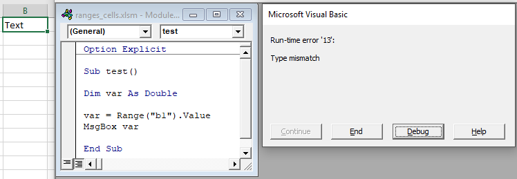
Dim var as Variant

var = Range("A1").Value
Here we used a variable of type Variant. Variant variables can accept any type of values. Instead, you could use a String variable type:
Dim var as String

var = Range("A1").Value
A String variable type will accept numerical values, but it will store the numbers as text.
If you know your cell value will be numerical, you could use a Double variable type (Double variables can store decimal values):
Dim var as Double

var = Range("A1").Value
However, if you attempt to store a cell value containing text in a double variable, you will receive an type mismatch error:
Other Cell Value Examples
VBA Programming | Code Generator does work for you!
Copy Cell Value
It’s easy to set a cell value equal to another cell value (or “Copy” a cell value):
Range("A1").Value = Range("B1").ValueYou can even do this with ranges of cells (the ranges must be the same size):
Range("A1:A5").Value = Range("B1:B5").ValueCompare Cell Values
You can compare cell values using the standard comparison operators.
Test if cell values are equal:
MsgBox Range("A1").Value = Range("B1").ValueWill return TRUE if cell values are equal. Otherwise FALSE.
You can also create an If Statement to compare cell values:
If Range("A1").Value > Range("B1").Value Then

  Range("C1").Value = "Greater Than"

Elseif Range("A1").Value = Range("B1").Value Then

  Range("C1").Value = "Equal"

Else

  Range("C1").Value = "Less Than"

End If
You can compare text in the same way (Remember that VBA is Case Sensitive)
Set Range in Excel VBA
Set range in VBA means we specify a given range to the code or the procedure to execute. If we do not provide a specific range to a code, it will automatically assume the range from the worksheet with the active cell. So, it is very important in the code to have a range variable set.
After working with Excel for so many years, you must have understood that all works we do are on the worksheet. In worksheets, it is cells containing the data. So when you want to play around with data, you must be a behavior pattern of cells in worksheets. So, when the multiple cells get together, it becomes a RANGE. Therefore, to learn VBA, you should know everything about cells and ranges. So in this article, we will show you how to set the range of cells we can use for VBA codingVBA code refers to a set of instructions written by the user in the Visual Basic Applications programming language on a Visual Basic Editor (VBE) to perform a specific task.read more in detail.
Table of contents
- Set Range in Excel VBA
- How to Access Range of Cells in Excel VBA?
- Accessing Multiple Cells & Setting Range Reference in VBA
- Things to Remember
- Recommended Articles
You are free to use this image on your website, templates, etc, Please provide us with an attribution linkArticle Link to be Hyperlinked
For eg:
Source: VBA Set Range (wallstreetmojo.com)
What is the Range Object?
Range in VBA refers to an object. A range can contain a single cell, multiple cells, a row or column, etc.
In VBA, we can classify the range as below.
“Application >>> Workbook >>> Worksheet >>> Range”
First, we need to access the Application. Then under this, we need to refer to which workbook we are referring to. Next, in the workbook, we are referring to which worksheet we are referring to. Then in the worksheet, we need to mention the range of cells.
Using the Range of cells, we can enter the value to the cell or cells, we can read or get values from the cell or cells, we can delete, we can format, and we can do many other things as well.
How to Access the Range of Cells in Excel VBA?
You can download this VBA Set Range Excel Template here – VBA Set Range Excel Template
In VBA coding, we can refer to the cell using the VBA CELLS propertyCells are cells of the worksheet, and in VBA, when we refer to cells as a range property, we refer to the same cells. In VBA concepts, cells are also the same, no different from normal excel cells.read more and RANGE object. So, for example, if you want to refer to cell A1, we will first see using the RANGE object.
Inside the subprocedure, we need first to open the RANGE object.
Code:
Sub Range_Examples()

 Range(

End Sub

As you can see above, the RANGE object asks what cell we are referring to. So, we need to enter the cell address in double quotes.
Code:
Sub Range_Examples()

 Range ("A1")

End Sub

Once we supply the cell address, we must decide what to do with this cell using properties and methods. Now, put a dot to see the properties and methods of the RANGE object.

If we want to insert the value into the cell, we must choose the “Value” property.
Code:
Sub Range_Examples()

 Range("A1").Value

End Sub

To set a value, we need to put an equal sign and enter the value we want to insert into cell A1.
Code:
Sub Range_Examples()

 Range("A1").Value = "Excel VBA Class"

End Sub

Run the code through the run option and see the magic in cell A1.

As the code mentioned, we have the value in cell A1.
Similarly, we can also refer to the cell using the CELLS property. Open the CELLS property and see the syntax.

It is unlike the RANGE object, where we can enter the cell address directly in double quotes. Rather, we need to give a row number and column to refer to the cell. For example, since we are referring to cell A1, we can say the row is 1, and the column is 1.

After mentioning the cell address, we can use properties and methods to work with cells. But the problem here is unlike the Range object after putting a dot. We do not get to see the IntelliSense list.

So, it would help if you were an expert to refer to the cells using the CELLS property.
Code:
Sub CELLS_Examples()

 Cells(1, 1).Value = "Excel VBA Class"

End Sub

Accessing Multiple Cells & Setting Range Reference in VBA
One of the big differences between CELLS and RANGE is using CELLS. We can access only one cell but using RANGE. We can access multiple cells, as well.
For example, for cells A1 to B5, if we want the value of 50, we can write the code below.
Code:
Sub Range_Examples()

 Range("A1:B5").Value = 50

End Sub

It will insert the value of 50 from cells A1 to B5.

Instead of referring to the cells directly, we can use the variable to hold the reference of specific cells.
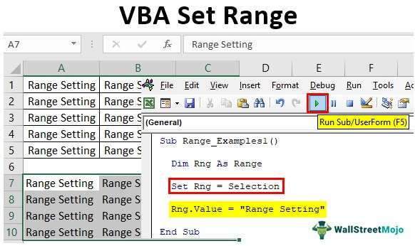
First, define the variable as the “Range” object.
Code:
Sub Range_Examples()

  Dim Rng As Range

End Sub

Once we define the variable as the “Range” object, we need to set the reference for this variable about what the cell addresses will hold the reference to.
To set the reference, we need to use the “SET” keyword and enter the cell addresses using the RANGE object.
Code:
Sub Range_Examples()

  Dim Rng As Range

  Set Rng = Range("A1:B5")

End Sub

The variable “Rng” refers to the cells A1 to B5.
Instead of writing the cell address Range (“A1:B5”), we can use the variable name “Rng.”
Code:
Sub Range_Examples()

  Dim Rng As Range

  Set Rng = Range("A1:B5")

  Rng.Value = "Range Setting"

End Sub

It will insert the mentioned value from the A1 to the B5 cells.

Assume you want whatever the selected cell should be a reference, then we can set the reference as follows.
Code:
Sub Range_Examples()

  Dim Rng As Range

  Set Rng = Selection

  Rng.Value = "Range Setting"

End Sub

This one is a beauty because if we select any of the cells and run it, it will also insert the value to those cells.
For example, we will select certain cells.

Now, we will execute the code and see what happens.

For all the selected cells, it has inserted the value.
Like this, we can set the range reference by declaring variables in VBAVariable declaration is necessary in VBA to define a variable for a specific data type so that it can hold values; any variable that is not defined in VBA cannot hold values.read more.
Things to Remember
- The range can select multiple cells, but CELLS can select one cell at a time.
- RANGE is an object, and CELLS is property.
- Any object variable should be the object’s reference using the SET keyword.
Recommended Articles
This article is a guide to VBA Set Range. Here, we discuss setting the range of Excel cells used for reference through VBA code, examples, and a downloadable Excel template. Below you can find some useful Excel VBA articles: –
- VBA Set
- VBA Sort Option
- Range Cells in VBA
- Using Range Objects in VBA
- VBA INT
Свойство Cells объекта Range в VBA Excel, представляющее коллекцию ячеек заданного диапазона. Обращение к ячейкам диапазона с помощью свойства Cells.
Range.Cells – свойство, возвращающее коллекцию всех ячеек указанного диапазона.
Свойство Cells объекта Worksheet
Обращение к ячейке «A1» активного рабочего листа с помощью свойства Cells:
|
‘по индексу (порядковому номеру) ячейки MsgBox Cells(1).Address ‘Результат: $A$1 ‘по номеру строки и номеру столбца MsgBox Cells(1, 1).Address ‘Результат: $A$1 ‘по номеру строки и буквенному обозначению столбца MsgBox Cells(1, «A»).Address ‘Результат: $A$1 |
В данном случае в качестве объекта Range выступает диапазон всего активного рабочего листа (ActiveSheet). Полный путь к ячейке «A1» можно записать так:
|
MsgBox ThisWorkbook.ActiveSheet.Cells(1).Address ‘Результат: $A$1 MsgBox ThisWorkbook.ActiveSheet.Cells(1, 1).Address ‘Результат: $A$1 MsgBox ThisWorkbook.ActiveSheet.Cells(1, «A»).Address ‘Результат: $A$1 |
Обращение в VBA Excel к ячейке «C5» с помощью свойства Cells по имени рабочего листа (Worksheet) в другой книге Excel:
|
MsgBox Workbooks(«Книга1.xlsm»).Worksheets(«Лист1»).Cells(65539).Address ‘Результат: $C$5 в Excel 2016 MsgBox Workbooks(«Книга1.xlsm»).Worksheets(«Лист1»).Cells(5, 3).Address ‘Результат: $C$5 MsgBox Workbooks(«Книга1.xlsm»).Worksheets(«Лист1»).Cells(5, «C»).Address ‘Результат: $C$5 |
Обращение к диапазону «C5:G10» с помощью свойства Cells активного рабочего листа:
|
MsgBox Range(Cells(5, 3), Cells(10, 7)).Address ‘Результат: $C$5:$G$10 |
Обращение в VBA Excel к ячейкам заданного диапазона с помощью свойства Cells рассмотрим на коллекции ячеек диапазона «C5:G10». Обращаться будем к ячейке «D8» активного листа:
|
MsgBox Range(«C5:G10»).Cells(17).Address ‘Результат: $D$8 MsgBox Range(«C5:G10»).Cells(4, 2).Address ‘Результат: $D$8 MsgBox Range(«C5:G10»).Cells(4, «B»).Address ‘Результат: $D$8 |
Обратите внимание, что отсчет номеров строк, номеров и буквенных обозначений столбцов для указания адреса ячейки внутри диапазона ведется от верхней левой ячейки данного диапазона.
Обход диапазона ячеек циклом
Обход ячеек циклом For Each… Next
Обход ячеек циклом For Each… Next — это самый простой способ обхода всех ячеек заданного диапазона. Он может быть применен, например, для присвоения ячейкам свойств и значений или поиска ячейки с определенным свойством или значением.
Присвоение ячейкам диапазона «B3:F10» числовых значений, соответствующих их порядковым номерам (индексам) в диапазоне:
|
Sub Primer1() Dim myCell As Range, n As Long For Each myCell In Range(«B3:F10») n = n + 1 myCell = n Next End Sub |
Поиск в диапазоне «B3:F10», заполненном предыдущим кодом VBA Excel значениями, ячейки со значением «27», окрашивание ее в зеленый цвет и выход из цикла:
|
Sub Primer2() Dim myCell As Range, n As Long For Each myCell In Range(«B3:F10») If myCell = 27 Then myCell.Interior.Color = vbGreen Exit For End If Next End Sub |
Обход диапазона циклом For… Next
Цикл For… Next позволяет указывать переменные в качестве индексов ячеек или номеров строк и столбцов для обхода ячеек заданного диапазона.
Присвоение ячейкам диапазона «B3:F10» числовых значений, соответствующих их порядковым номерам (индексам) в диапазоне, с помощью цикла For… Next:
|
Sub Primer3() Dim i As Long, n As Long With Range(«B3:F10») n = .Cells.Count For i = 1 To n .Cells(i) = i Next End With End Sub |
Если в блоке с оператором With вместо строки .Cells(i) = i указать строку без точки впереди — Cells(i) = i, то свойство Cells будет относиться не к диапазону Range("B3:F10"), а к рабочему листу (объекту ActiveSheet). В этом случае, порядковыми номерами будут заполнены первые 40 ячеек первой строки активного рабочего листа.
Применение в качестве параметров свойства Cells объекта Range переменных, задающих номера строк и номера столбцов указанного диапазона при обходе его ячеек циклом For… Next:
|
Sub Primer4() Dim i1 As Long, i2 As Long, r As Long, c As Long With Range(«B3:F10») r = .Rows.Count c = .Columns.Count For i1 = 1 To r For i2 = 1 To c .Cells(i1, i2) = (i1 — 1) * c + i2 Next Next End With End Sub |
Номер ячейки на рабочем листе
Определение порядкового номера (индекса) активной ячейки на рабочем листе Excel с помощью кода VBA:
|
Sub Primer5() Dim n As Double n = (ActiveCell.Row — 1) * CDbl(Cells.Columns.Count) + ActiveCell.Column MsgBox n End Sub |
Selecting a cell is one of the most basic things users do in Excel.
There are many different ways to select a cell in Excel – such as using the mouse or the keyboard (or a combination of both).
In this article, I would show you how to select multiple cells in Excel. These cells could all be together (contiguous) or separated (non-contiguous)
While this is quite simple, I’m sure you’ll pick up a couple of new tricks to help you speed up your work and be more efficient.
So let’s get started!
Select Multiple Cells (that are all contiguous)
If you know how to select one cell in Excel, I’m sure you also know how to select multiple cells.
But let me still cover this anyway.
Suppose you want to select cells A1:D10.
Below are the steps to do this:
- Place the cursor on cell A1
- Select cell A1 (by using the left mouse button). Keep the mouse button pressed.
- Drag the cursor till cell D10 (so that it covers all the cells between A1 and D10)
- Leave the mouse button

Easy-peasy, right?
Now let’s see some more cases.
Select Rows/Columns
A lot of times, you will be required to select an entire row or column (or even multiple rows or columns). These could be to hide or delete these rows/columns, move it around in the worksheet, highlight it, etc.
Just like you can select a cell in Excel by placing the cursor and clicking the mouse, you can also select a row or a column by simply clicking on the row number or column alphabet.
Let’s go through each of these cases.
Select a Single Row/Column
Here is how you can select an entire row in Excel:
- Bring the cursor over the row number of the row that you want to select

- Use the left mouse-click to select the entire row


When you select the entire row, you will see that the color of that selection changes (it becomes a bit darker as compared to the rest of the cell in the worksheet).
Just like we have selected a row in Excel, you can also select a column (where instead of clicking on the row number, you have to click on the column alphabet, which is at the top of the column).
Also read: Select Till End of Data in a Column in Excel (Shortcuts)
Select Multiple Rows/Columns
Now, what if you don’t want to select just one row.
What if you want to select multiple rows?
For example, let’s say that you want to select row number 2, 3, and 4 at the same time.
Here is how to do that:
- Place the cursor over row number 2 in the worksheet
- Press the mouse left button while your cursor is on row number two (keep the mouse button pressed)
- Keep the mouse left-button still pressed and drag the cursor down till row 4
- Leave the mouse button

You’ll see that this would select three adjacent rows that you covered through your mouse.
Just like we have selected three adjacent rows, you can follow the same steps to select multiple columns as well.
Select Multiple Non-Adjacent Rows/Columns
What if you want to select multiple rows, but these are not-adjacent.
For example, you may want to select row numbers 2, 4, 7.
In such a case you cannot use the mouse drag technique covered above because it would select all the rows in between.
To do this, you will have to use a combination of keyboard and mouse.
Here is how to select non-adjacent multiple rows in Excel:
- Place the cursor over row number 2 in the worksheet
- Hold the Control key on your keyboard
- Press the mouse left button while your cursor is on row number 2
- Leave the mouse button
- Place the cursor over the next row you want to select (row 4 in this case),
- Hold the Control key on your keyboard
- Press the mouse left button while your cursor is on row number 4. Once row 4 is also selected, leave the mouse button
- Repeat the same to select row 7 as well
- Leave the Control key

The above steps would select multiple non-adjacent rows in the worksheet.
You can use the same method to select multiple non-adjacent columns.
Select All the Cells in the Current Table/Data
Most of the time, when you have to select multiple cells in Excel, these would be the cells in a specific table or a dataset.
You can do this by using a simple keyboard shortcut.
Below are the steps to select all the cells in the current table:
- Select any cell within the data set

- Hold the Ctrl key and then press the A key


The above steps would select all the cells in the data set (where Excel considers this data set to extend until it encounters a blank row or column).
As soon as Excel encounters a blank row or blank column, it would consider this as the end of the data set (so anything beyond the blank row/column will not be selected)
Select All the Cells in the Worksheet
Another common task that is often done is to select all the cells in the worksheet.
I often work with data downloaded from different databases, and often this data is formatted in a certain way. And my first step as soon as I get this data is to select all the cells and remove all the formatting.
Here is how you can select all the cells in the active worksheet:
- Select the worksheet in which you want to select all the cells
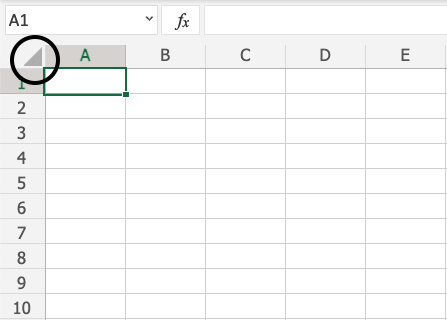
- Click on the small inverted triangle at the top left part of the worksheet


This would instantly select all the cells in the entire worksheet (note that this would not select any object such as a chart or shape in the worksheet).
And if you are a keyboard shortcut aficionado, you can use the below shortcut:
Control + A + A (hold the control key and press the A key twice)
If you have selected a blank cell that does not have any data around it, you don’t need to press the A key twice (just use Control-A).
Select Multiple Non-Contiguous Cells
The more you work with Excel, the more you would have a need to select multiple non-contiguous cells (such as A2, A4, A7, etc.)
Below I have an example where I only want to select the records for the US. And since these are not adjacent to each other, I somehow need to figure out how to select all these multiple cells at the same time.

Again, you can do this easily using a combination of keyboard and mouse.
Below are the steps to do this:
- Hold the Control key on the keyboard
- One by one, select all the non-contiguous cells (or range of cells) that you want to remain selected
- When done, leave the Control key

The above technique also works when you want to select non-contiguous rows or columns. You can simply hold the Control key and select the non-adjacent rows/columns.
Select Cells Using Name Box
So far we have seen examples where we could manually select the cells because they were close by.
But in some cases, you may have to select multiple cells or rows/columns that are far off in the worksheet.
Of course, you can do that manually, but you’ll soon realize that it’s time-consuming and error-prone.
If it’s something you have to do quite often (that is, select the same cells or rows/columns), you can use the Name Box to do it a lot faster.
Name Box is the small field that you have on the left of the formula bar in Excel.

When you type a cell reference (or a range reference) in the name box, it selects all the specified cells.
For example, let’s say I want to select cell A1, K3, and M20
Since these are quite far off, if I try and select these using the mouse, I would have to scroll a little bit.
This may be justified if you only have to do it once in a while, but in case you have to say select the same cells often, you can use the name box instead.
Below are the steps to select multiple cells using the name box:
- Click on the name box
- Enter the cell references that you want to select (separated by comma)

- Hit the enter key

The above steps would instantly select all the cells that you have entered in the name box.
Of these selected cells, one would be the active cell (and the cell reference of the active cell would now be visible in the name box).
Select a Named Range
If you have created a named range in Excel, you can also use the Name Box to refer to the entire named range (instead of using the cell references as shown in the method above)
If you don’t know what a Named Range is, it’s when you assign a name to a cell or a range of cells and then use the name instead of the cell reference in formulas.
Below are the steps to quickly create a Named Range in Excel:
- Select the cells that you want to be included in the Named Range
- Click on the Name box (which is the field adjacent to the formula bar)
- Enter the name that you want to assign to the selected range of cells (you can’t have spaces in the name)

- Hit the Enter key

The above steps would create a Named Range for the cells that you selected.
Now, if you want to quickly select these same cells, instead of doing that manually you can simply go to the Name box and enter the name of the named range (or click on the dropdown icon and select the name from there)

This would instantly select all the cells that are part of that Named Range.
So, these are some of the methods that you can use to select multiple cells in Excel.
I hope you found this tutorial useful.
Other Excel tutorials you may like:
- How to Select Non-adjacent cells in Excel?
- How to Deselect Cells in Excel
- 3 Quick Ways to Select Visible Cells in Excel
- How to Select Every Third Row in Excel (or select every Nth Row)
- How to Quickly Select Blank Cells in Excel
- How to Select Entire Column (or Row) in Excel
- How to Select Every Other Row in Excel
“It is a capital mistake to theorize before one has data”- Sir Arthur Conan Doyle
This post covers everything you need to know about using Cells and Ranges in VBA. You can read it from start to finish as it is laid out in a logical order. If you prefer you can use the table of contents below to go to a section of your choice.
Topics covered include Offset property, reading values between cells, reading values to arrays and formatting cells.
A Quick Guide to Ranges and Cells
| Function | Takes | Returns | Example | Gives |
|---|---|---|---|---|
|
Range |
cell address | multiple cells | .Range(«A1:A4») | $A$1:$A$4 |
| Cells | row, column | one cell | .Cells(1,5) | $E$1 |
| Offset | row, column | multiple cells | Range(«A1:A2») .Offset(1,2) |
$C$2:$C$3 |
| Rows | row(s) | one or more rows | .Rows(4) .Rows(«2:4») |
$4:$4 $2:$4 |
| Columns | column(s) | one or more columns | .Columns(4) .Columns(«B:D») |
$D:$D $B:$D |
Download the Code
The Webinar
If you are a member of the VBA Vault, then click on the image below to access the webinar and the associated source code.
(Note: Website members have access to the full webinar archive.)

Introduction
This is the third post dealing with the three main elements of VBA. These three elements are the Workbooks, Worksheets and Ranges/Cells. Cells are by far the most important part of Excel. Almost everything you do in Excel starts and ends with Cells.
Generally speaking, you do three main things with Cells
- Read from a cell.
- Write to a cell.
- Change the format of a cell.
Excel has a number of methods for accessing cells such as Range, Cells and Offset.These can cause confusion as they do similar things and can lead to confusion
In this post I will tackle each one, explain why you need it and when you should use it.
Let’s start with the simplest method of accessing cells – using the Range property of the worksheet.
Important Notes
I have recently updated this article so that is uses Value2.
You may be wondering what is the difference between Value, Value2 and the default:
' Value2
Range("A1").Value2 = 56

' Value
Range("A1").Value = 56

' Default uses value
Range("A1") = 56
Using Value may truncate number if the cell is formatted as currency. If you don’t use any property then the default is Value.
It is better to use Value2 as it will always return the actual cell value(see this article from Charle Williams.)
The Range Property
The worksheet has a Range property which you can use to access cells in VBA. The Range property takes the same argument that most Excel Worksheet functions take e.g. “A1”, “A3:C6” etc.
The following example shows you how to place a value in a cell using the Range property.
' https://excelmacromastery.com/
Public Sub WriteToCell()

    ' Write number to cell A1 in sheet1 of this workbook
    ThisWorkbook.Worksheets("Sheet1").Range("A1").Value2 = 67

    ' Write text to cell A2 in sheet1 of this workbook
    ThisWorkbook.Worksheets("Sheet1").Range("A2").Value2 = "John Smith"

    ' Write date to cell A3 in sheet1 of this workbook
    ThisWorkbook.Worksheets("Sheet1").Range("A3").Value2 = #11/21/2017#

End Sub
As you can see Range is a member of the worksheet which in turn is a member of the Workbook. This follows the same hierarchy as in Excel so should be easy to understand. To do something with Range you must first specify the workbook and worksheet it belongs to.
For the rest of this post I will use the code name to reference the worksheet.

The following code shows the above example using the code name of the worksheet i.e. Sheet1 instead of ThisWorkbook.Worksheets(“Sheet1”).
' https://excelmacromastery.com/
Public Sub UsingCodeName()

    ' Write number to cell A1 in sheet1 of this workbook
    Sheet1.Range("A1").Value2 = 67

    ' Write text to cell A2 in sheet1 of this workbook
    Sheet1.Range("A2").Value2 = "John Smith"

    ' Write date to cell A3 in sheet1 of this workbook
    Sheet1.Range("A3").Value2 = #11/21/2017#

End Sub
You can also write to multiple cells using the Range property
' https://excelmacromastery.com/
Public Sub WriteToMulti()

    ' Write number to a range of cells
    Sheet1.Range("A1:A10").Value2 = 67

    ' Write text to multiple ranges of cells
    Sheet1.Range("B2:B5,B7:B9").Value2 = "John Smith"

End Sub
You can download working examples of all the code from this post from the top of this article.
The Cells Property of the Worksheet
The worksheet object has another property called Cells which is very similar to range. There are two differences
- Cells returns a range of one cell only.
- Cells takes row and column as arguments.
The example below shows you how to write values to cells using both the Range and Cells property
' https://excelmacromastery.com/
Public Sub UsingCells()

    ' Write to A1
    Sheet1.Range("A1").Value2 = 10
    Sheet1.Cells(1, 1).Value2  = 10

    ' Write to A10
    Sheet1.Range("A10").Value2 = 10
    Sheet1.Cells(10, 1).Value2  = 10

    ' Write to E1
    Sheet1.Range("E1").Value2 = 10
    Sheet1.Cells(1, 5).Value2  = 10

End Sub
You may be wondering when you should use Cells and when you should use Range. Using Range is useful for accessing the same cells each time the Macro runs.
For example, if you were using a Macro to calculate a total and write it to cell A10 every time then Range would be suitable for this task.
Using the Cells property is useful if you are accessing a cell based on a number that may vary. It is easier to explain this with an example.
In the following code, we ask the user to specify the column number. Using Cells gives us the flexibility to use a variable number for the column.
' https://excelmacromastery.com/
Public Sub WriteToColumn()

    Dim UserCol As Integer

    ' Get the column number from the user
    UserCol = Application.InputBox(" Please enter the column...", Type:=1)

    ' Write text to user selected column
    Sheet1.Cells(1, UserCol).Value2 = "John Smith"

End Sub
In the above example, we are using a number for the column rather than a letter.
To use Range here would require us to convert these values to the letter/number cell reference e.g. “C1”. Using the Cells property allows us to provide a row and a column number to access a cell.
Sometimes you may want to return more than one cell using row and column numbers. The next section shows you how to do this.
Using Cells and Range together
As you have seen you can only access one cell using the Cells property. If you want to return a range of cells then you can use Cells with Ranges as follows
' https://excelmacromastery.com/
Public Sub UsingCellsWithRange()

    With Sheet1
        ' Write 5 to Range A1:A10 using Cells property
        .Range(.Cells(1, 1), .Cells(10, 1)).Value2 = 5

        ' Format Range B1:Z1 to be bold
        .Range(.Cells(1, 2), .Cells(1, 26)).Font.Bold = True

    End With

End Sub
As you can see, you provide the start and end cell of the Range. Sometimes it can be tricky to see which range you are dealing with when the value are all numbers. Range has a property called Address which displays the letter/ number cell reference of any range. This can come in very handy when you are debugging or writing code for the first time.
In the following example we print out the address of the ranges we are using:
' https://excelmacromastery.com/
Public Sub ShowRangeAddress()

    ' Note: Using underscore allows you to split up lines of code
    With Sheet1

        ' Write 5 to Range A1:A10 using Cells property
        .Range(.Cells(1, 1), .Cells(10, 1)).Value2 = 5
        Debug.Print "First address is : " _
            + .Range(.Cells(1, 1), .Cells(10, 1)).Address

        ' Format Range B1:Z1 to be bold
        .Range(.Cells(1, 2), .Cells(1, 26)).Font.Bold = True
        Debug.Print "Second address is : " _
            + .Range(.Cells(1, 2), .Cells(1, 26)).Address

    End With

End Sub
In the example I used Debug.Print to print to the Immediate Window. To view this window select View->Immediate Window(or Ctrl G)


You can download all the code for this post from the top of this article.
The Offset Property of Range
Range has a property called Offset. The term Offset refers to a count from the original position. It is used a lot in certain areas of programming. With the Offset property you can get a Range of cells the same size and a certain distance from the current range. The reason this is useful is that sometimes you may want to select a Range based on a certain condition. For example in the screenshot below there is a column for each day of the week. Given the day number(i.e. Monday=1, Tuesday=2 etc.) we need to write the value to the correct column.

We will first attempt to do this without using Offset.
' https://excelmacromastery.com/
' This sub tests with different values
Public Sub TestSelect()

    ' Monday
    SetValueSelect 1, 111.21
    ' Wednesday
    SetValueSelect 3, 456.99
    ' Friday
    SetValueSelect 5, 432.25
    ' Sunday
    SetValueSelect 7, 710.17

End Sub

' Writes the value to a column based on the day
Public Sub SetValueSelect(lDay As Long, lValue As Currency)

    Select Case lDay
        Case 1: Sheet1.Range("H3").Value2 = lValue
        Case 2: Sheet1.Range("I3").Value2 = lValue
        Case 3: Sheet1.Range("J3").Value2 = lValue
        Case 4: Sheet1.Range("K3").Value2 = lValue
        Case 5: Sheet1.Range("L3").Value2 = lValue
        Case 6: Sheet1.Range("M3").Value2 = lValue
        Case 7: Sheet1.Range("N3").Value2 = lValue
    End Select

End Sub
As you can see in the example, we need to add a line for each possible option. This is not an ideal situation. Using the Offset Property provides a much cleaner solution
' https://excelmacromastery.com/
' This sub tests with different values
Public Sub TestOffset()

    DayOffSet 1, 111.01
    DayOffSet 3, 456.99
    DayOffSet 5, 432.25
    DayOffSet 7, 710.17

End Sub

Public Sub DayOffSet(lDay As Long, lValue As Currency)

    ' We use the day value with offset specify the correct column
    Sheet1.Range("G3").Offset(, lDay).Value2 = lValue

End Sub
As you can see this solution is much better. If the number of days in increased then we do not need to add any more code. For Offset to be useful there needs to be some kind of relationship between the positions of the cells. If the Day columns in the above example were random then we could not use Offset. We would have to use the first solution.
One thing to keep in mind is that Offset retains the size of the range. So .Range(“A1:A3”).Offset(1,1) returns the range B2:B4. Below are some more examples of using Offset
' https://excelmacromastery.com/
Public Sub UsingOffset()

    ' Write to B2 - no offset
    Sheet1.Range("B2").Offset().Value2 = "Cell B2"

    ' Write to C2 - 1 column to the right
    Sheet1.Range("B2").Offset(, 1).Value2 = "Cell C2"

    ' Write to B3 - 1 row down
    Sheet1.Range("B2").Offset(1).Value2 = "Cell B3"

    ' Write to C3 - 1 column right and 1 row down
    Sheet1.Range("B2").Offset(1, 1).Value2 = "Cell C3"

    ' Write to A1 - 1 column left and 1 row up
    Sheet1.Range("B2").Offset(-1, -1).Value2 = "Cell A1"

    ' Write to range E3:G13 - 1 column right and 1 row down
    Sheet1.Range("D2:F12").Offset(1, 1).Value2 = "Cells E3:G13"

End Sub
Using the Range CurrentRegion
CurrentRegion returns a range of all the adjacent cells to the given range.
In the screenshot below you can see the two current regions. I have added borders to make the current regions clear.

A row or column of blank cells signifies the end of a current region.
You can manually check the CurrentRegion in Excel by selecting a range and pressing Ctrl + Shift + *.
If we take any range of cells within the border and apply CurrentRegion, we will get back the range of cells in the entire area.
For example
Range(“B3”).CurrentRegion will return the range B3:D14
Range(“D14”).CurrentRegion will return the range B3:D14
Range(“C8:C9”).CurrentRegion will return the range B3:D14
and so on
How to Use
We get the CurrentRegion as follows
' Current region will return B3:D14 from above example
Dim rg As Range
Set rg = Sheet1.Range("B3").CurrentRegion
Read Data Rows Only
Read through the range from the second row i.e.skipping the header row
' Current region will return B3:D14 from above example
Dim rg As Range
Set rg = Sheet1.Range("B3").CurrentRegion

' Start at row 2 - row after header
Dim i As Long
For i = 2 To rg.Rows.Count
    ' current row, column 1 of range
    Debug.Print rg.Cells(i, 1).Value2
Next i
Remove Header
Remove header row(i.e. first row) from the range. For example if range is A1:D4 this will return A2:D4
' Current region will return B3:D14 from above example
Dim rg As Range
Set rg = Sheet1.Range("B3").CurrentRegion

' Remove Header
Set rg = rg.Resize(rg.Rows.Count - 1).Offset(1)

' Start at row 1 as no header row
Dim i As Long
For i = 1 To rg.Rows.Count
    ' current row, column 1 of range
    Debug.Print rg.Cells(i, 1).Value2
Next i
Using Rows and Columns as Ranges
If you want to do something with an entire Row or Column you can use the Rows or Columns property of the Worksheet. They both take one parameter which is the row or column number you wish to access
' https://excelmacromastery.com/
Public Sub UseRowAndColumns()

    ' Set the font size of column B to 9
    Sheet1.Columns(2).Font.Size = 9

    ' Set the width of columns D to F
    Sheet1.Columns("D:F").ColumnWidth = 4

    ' Set the font size of row 5 to 18
    Sheet1.Rows(5).Font.Size = 18

End Sub
Using Range in place of Worksheet
You can also use Cells, Rows and Columns as part of a Range rather than part of a Worksheet. You may have a specific need to do this but otherwise I would avoid the practice. It makes the code more complex. Simple code is your friend. It reduces the possibility of errors.
The code below will set the second column of the range to bold. As the range has only two rows the entire column is considered B1:B2
' https://excelmacromastery.com/
Public Sub UseColumnsInRange()

    ' This will set B1 and B2 to be bold
    Sheet1.Range("A1:C2").Columns(2).Font.Bold = True

End Sub
You can download all the code for this post from the top of this article.
Reading Values from one Cell to another
In most of the examples so far we have written values to a cell. We do this by placing the range on the left of the equals sign and the value to place in the cell on the right. To write data from one cell to another we do the same. The destination range goes on the left and the source range goes on the right.
The following example shows you how to do this:
' https://excelmacromastery.com/
Public Sub ReadValues()

    ' Place value from B1 in A1
    Sheet1.Range("A1").Value2 = Sheet1.Range("B1").Value2

    ' Place value from B3 in sheet2 to cell A1
    Sheet1.Range("A1").Value2 = Sheet2.Range("B3").Value2

    ' Place value from B1 in cells A1 to A5
    Sheet1.Range("A1:A5").Value2 = Sheet1.Range("B1").Value2

    ' You need to use the "Value" property to read multiple cells
    Sheet1.Range("A1:A5").Value2 = Sheet1.Range("B1:B5").Value2

End Sub
As you can see from this example it is not possible to read from multiple cells. If you want to do this you can use the Copy function of Range with the Destination parameter
' https://excelmacromastery.com/
Public Sub CopyValues()

    ' Store the copy range in a variable
    Dim rgCopy As Range
    Set rgCopy = Sheet1.Range("B1:B5")

    ' Use this to copy from more than one cell
    rgCopy.Copy Destination:=Sheet1.Range("A1:A5")

    ' You can paste to multiple destinations
    rgCopy.Copy Destination:=Sheet1.Range("A1:A5,C2:C6")

End Sub
The Copy function copies everything including the format of the cells. It is the same result as manually copying and pasting a selection. You can see more about it in the Copying and Pasting Cells section.
Using the Range.Resize Method
When copying from one range to another using assignment(i.e. the equals sign), the destination range must be the same size as the source range.
Using the Resize function allows us to resize a range to a given number of rows and columns.
For example:
' https://excelmacromastery.com/
Sub ResizeExamples()

    ' Prints A1
    Debug.Print Sheet1.Range("A1").Address

    ' Prints A1:A2
    Debug.Print Sheet1.Range("A1").Resize(2, 1).Address

    ' Prints A1:A5
    Debug.Print Sheet1.Range("A1").Resize(5, 1).Address

    ' Prints A1:D1
    Debug.Print Sheet1.Range("A1").Resize(1, 4).Address

    ' Prints A1:C3
    Debug.Print Sheet1.Range("A1").Resize(3, 3).Address

End Sub
When we want to resize our destination range we can simply use the source range size.
In other words, we use the row and column count of the source range as the parameters for resizing:
' https://excelmacromastery.com/
Sub Resize()

    Dim rgSrc As Range, rgDest As Range

    ' Get all the data in the current region
    Set rgSrc = Sheet1.Range("A1").CurrentRegion

      ' Get the range destination
    Set rgDest = Sheet2.Range("A1")
    Set rgDest = rgDest.Resize(rgSrc.Rows.Count, rgSrc.Columns.Count)

    rgDest.Value2 = rgSrc.Value2

End Sub
We can do the resize in one line if we prefer:
' https://excelmacromastery.com/
Sub ResizeOneLine()

    Dim rgSrc As Range

    ' Get all the data in the current region
    Set rgSrc = Sheet1.Range("A1").CurrentRegion

    With rgSrc
        Sheet2.Range("A1").Resize(.Rows.Count, .Columns.Count).Value2 = .Value2
    End With

End Sub
Reading Values to variables
We looked at how to read from one cell to another. You can also read from a cell to a variable. A variable is used to store values while a Macro is running. You normally do this when you want to manipulate the data before writing it somewhere. The following is a simple example using a variable. As you can see the value of the item to the right of the equals is written to the item to the left of the equals.
' https://excelmacromastery.com/
Public Sub UseVariables()

    ' Create
    Dim number As Long

    ' Read number from cell
    number = Sheet1.Range("A1").Value2

    ' Add 1 to value
    number = number + 1

    ' Write new value to cell
    Sheet1.Range("A2").Value2 = number

End Sub
To read text to a variable you use a variable of type String:
' https://excelmacromastery.com/
Public Sub UseVariableText()

    ' Declare a variable of type string
    Dim text As String

    ' Read value from cell
    text = Sheet1.Range("A1").Value2

    ' Write value to cell
    Sheet1.Range("A2").Value2 = text

End Sub
You can write a variable to a range of cells. You just specify the range on the left and the value will be written to all cells in the range.
' https://excelmacromastery.com/
Public Sub VarToMulti()

    ' Read value from cell
    Sheet1.Range("A1:B10").Value2 = 66

End Sub
You cannot read from multiple cells to a variable. However you can read to an array which is a collection of variables. We will look at doing this in the next section.
How to Copy and Paste Cells
If you want to copy and paste a range of cells then you do not need to select them. This is a common error made by new VBA users.
Note: We normally use Range.Copy when we want to copy formats, formulas, validation. If we want to copy values it is not the most efficient method.
I have written a complete guide to copying data in Excel VBA here.
You can simply copy a range of cells like this:
Range("A1:B4").Copy Destination:=Range("C5")
Using this method copies everything – values, formats, formulas and so on. If you want to copy individual items you can use the PasteSpecial property of range.
It works like this
Range("A1:B4").Copy
Range("F3").PasteSpecial Paste:=xlPasteValues
Range("F3").PasteSpecial Paste:=xlPasteFormats
Range("F3").PasteSpecial Paste:=xlPasteFormulas
The following table shows a full list of all the paste types
| Paste Type |
|---|
| xlPasteAll |
| xlPasteAllExceptBorders |
| xlPasteAllMergingConditionalFormats |
| xlPasteAllUsingSourceTheme |
| xlPasteColumnWidths |
| xlPasteComments |
| xlPasteFormats |
| xlPasteFormulas |
| xlPasteFormulasAndNumberFormats |
| xlPasteValidation |
| xlPasteValues |
| xlPasteValuesAndNumberFormats |
Reading a Range of Cells to an Array
You can also copy values by assigning the value of one range to another.
Range("A3:Z3").Value2 = Range("A1:Z1").Value2
The value of range in this example is considered to be a variant array. What this means is that you can easily read from a range of cells to an array. You can also write from an array to a range of cells. If you are not familiar with arrays you can check them out in this post.
The following code shows an example of using an array with a range:
' https://excelmacromastery.com/
Public Sub ReadToArray()

    ' Create dynamic array
    Dim StudentMarks() As Variant

    ' Read 26 values into array from the first row
    StudentMarks = Range("A1:Z1").Value2

    ' Do something with array here

    ' Write the 26 values to the third row
    Range("A3:Z3").Value2 = StudentMarks

End Sub
Keep in mind that the array created by the read is a 2 dimensional array. This is because a spreadsheet stores values in two dimensions i.e. rows and columns
Going through all the cells in a Range
Sometimes you may want to go through each cell one at a time to check value.
You can do this using a For Each loop shown in the following code
' https://excelmacromastery.com/
Public Sub TraversingCells()

    ' Go through each cells in the range
    Dim rg As Range
    For Each rg In Sheet1.Range("A1:A10,A20")
        ' Print address of cells that are negative
        If rg.Value < 0 Then
            Debug.Print rg.Address + " is negative."
        End If
    Next

End Sub
You can also go through consecutive Cells using the Cells property and a standard For loop.
The standard loop is more flexible about the order you use but it is slower than a For Each loop.
' https://excelmacromastery.com/
Public Sub TraverseCells()

    ' Go through cells from A1 to A10
    Dim i As Long
    For i = 1 To 10
        ' Print address of cells that are negative
        If Range("A" & i).Value < 0 Then
            Debug.Print Range("A" & i).Address + " is negative."
        End If
    Next

    ' Go through cells in reverse i.e. from A10 to A1
    For i = 10 To 1 Step -1
        ' Print address of cells that are negative
        If Range("A" & i) < 0 Then
            Debug.Print Range("A" & i).Address + " is negative."
        End If
    Next

End Sub
Formatting Cells
Sometimes you will need to format the cells the in spreadsheet. This is actually very straightforward. The following example shows you various formatting you can add to any range of cells
' https://excelmacromastery.com/
Public Sub FormattingCells()

    With Sheet1

        ' Format the font
        .Range("A1").Font.Bold = True
        .Range("A1").Font.Underline = True
        .Range("A1").Font.Color = rgbNavy

        ' Set the number format to 2 decimal places
        .Range("B2").NumberFormat = "0.00"
        ' Set the number format to a date
        .Range("C2").NumberFormat = "dd/mm/yyyy"
        ' Set the number format to general
        .Range("C3").NumberFormat = "General"
        ' Set the number format to text
        .Range("C4").NumberFormat = "Text"

        ' Set the fill color of the cell
        .Range("B3").Interior.Color = rgbSandyBrown

        ' Format the borders
        .Range("B4").Borders.LineStyle = xlDash
        .Range("B4").Borders.Color = rgbBlueViolet

    End With

End Sub
Main Points
The following is a summary of the main points
- Range returns a range of cells
- Cells returns one cells only
- You can read from one cell to another
- You can read from a range of cells to another range of cells.
- You can read values from cells to variables and vice versa.
- You can read values from ranges to arrays and vice versa
- You can use a For Each or For loop to run through every cell in a range.
- The properties Rows and Columns allow you to access a range of cells of these types
What’s Next?
Free VBA Tutorial If you are new to VBA or you want to sharpen your existing VBA skills then why not try out the The Ultimate VBA Tutorial.
Related Training: Get full access to the Excel VBA training webinars and all the tutorials.
(NOTE: Planning to build or manage a VBA Application? Learn how to build 10 Excel VBA applications from scratch.)
One of the basic things you need to do in Excel VBA is to select a specific range to do something with it. This article will show you how to use Range, Cells, Offset and Resize to select a range in Excel VBA.
Select all the cells of a worksheet
Cells.SelectSelect a cell
Cells(4, 5).Select=
Range("E4").SelectIt seems Range() is much easier to read and Cells() is easier to use inside a loop.
Select a set of contiguous cells
Range("C3:G8").Select=
Range(Cells(3, 3), Cells(8, 7)).Select=
Range("C3", "G8").SelectSelect a set of non contiguous cells
Range("A2,A4,B5").SelectSelect a set of non contiguous cells and a range
Range("A2,A4,B5:B8").SelectSelect a named range
Range("MyRange").Select=
Application.Goto "MyRange"Select an entire row
Range("1:1").SelectSelect an entire column
Range("A:A").SelectSelect the last cell of a column of contiguous data
Range("A1").End(xlDown).SelectWhen this code is used with the following example table, cell A3 will be selected.
Select the blank cell at bottom of a column of contiguous data
Range("A1").End(xlDown).Offset(1,0).SelectWhen this code is used with the following example table, cell A4 will be selected.
Select an entire range of contiguous cells in a column
Range("A1", Range("A1").End(xlDown)).SelectWhen this code is used with the following example table, range A1:A3 will be selected.
Select an entire range of non-contiguous cells in a column
Range("A1", Range("A" & Rows.Count).End(xlUp)).SelectNote: This VBA code supports Excel 2003 to 2013.
When this code is used with the following example table, range A1:A8 will be selected.
Select a rectangular range of cells around a cell
Range("A1").CurrentRegion.SelectSelect a cell relative to another cell
ActiveCell.Offset(5, 5).SelectRange("D3").Offset(5, -1).SelectSelect a specified range, offset It, and then resize It
Range("A1").Offset(3, 2).Resize(3, 3).SelectWhen this code is used with the following example table, range C4:E6 will be selected.
Ranges
Range is an important part of Excel because it allows you to work with selections of cells.
There are four different operations for selection;
- Selecting a cell
- Selecting multiple cells
- Selecting a column
- Selecting a row
Before having a look at the different operations for selection, we will introduce the Name Box.
The Name Box
The Name Box shows you the reference of which cell or range you have selected. It can also be used to select cells or ranges by typing their values.
You will learn more about the Name Box later in this chapter.
Selecting a Cell
Cells are selected by clicking them with the left mouse button or by navigating to them with the keyboard arrows.
It is easiest to use the mouse to select cells.
To select cell A1, click on it:
Selecting Multiple Cells
More than one cell can be selected by pressing and holding down CTRL or Command and left clicking the cells. Once finished with selecting, you can let go of CTRL or Command.
Lets try an example: Select the cells A1, A7, C1, C7 and B4.
Did it look like the picture below?
Selecting a Column
Columns are selected by left clicking it. This will select all cells in the sheet related to the column.
To select column A, click on the letter A in the column bar:
Selecting a Row
Rows are selected by left clicking it. This will select all the cells in the sheet related to that row.
To select row 1, click on its number in the row bar:
Selecting the Entire Sheet
The entire spreadsheet can be selected by clicking the triangle in the top-left corner of the spreadsheet: ![]()
Now, the whole spreadsheet is selected:
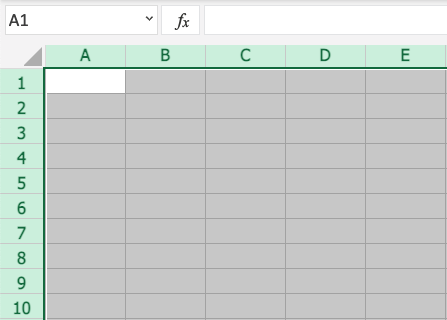
Note: You can also select the entire spreadsheet by pressing Ctrl+A for Windows, or Cmd+A for MacOS.
Selection of Ranges
Selection of cell ranges has many use areas and it is one of the most important concepts of Excel. Do not think too much about how it is used with values. You will learn about this in a later chapter. For now let’s focus on how to select ranges.
There are two ways to select a range of cells
- Name Box
- Drag to mark a range.
The easiest way is drag and mark. Let’s keep it simple and start there.
How to drag and mark a range, step-by-step:
- Select a cell
- Left click it and hold the mouse button down
- Move your mouse pointer over the range that you want selected. The range that is marked will turn grey.
- Let go of the mouse button when you have marked the range
Let’s have a look at an example for how to mark the range A1:E10.
Note: You will learn about why the range is called A1:E10 after this example.
Select cell A1:
Press and hold A1 with the left mouse button. Move to the mouse pointer to mark the selection range. The grey area helps us to see the covered range.
Let go of the left mouse button when you have marked the range A1:E10:
You have successfully selected the range A1:E10. Well done!
The second way to select a range is to enter the range values in the Name Box. The range is set by first entering the cell reference for the top left corner, then the bottom right corner. The range is made using those two as coordinates. That is why the cell range has the reference of two cells and the
: in between.
Top left corner reference : Right bottom corner reference
The range shown in the picture has the value of A1:E10:
The best way for now is to use the drag and mark method as it is easier and more visual.
In the next chapter you will learn about filling and how this applies to the ranges that we have just learned.