
Excel for Microsoft 365 Excel for Microsoft 365 for Mac Excel for the web Excel 2021 Excel 2021 for Mac Excel 2019 Excel 2019 for Mac Excel 2016 Excel 2016 for Mac Excel 2013 Excel 2010 Excel 2007 Excel for Mac 2011 Excel Starter 2010 More…Less
This article describes the formula syntax and usage of the OFFSET function in Microsoft Excel.
Description
Returns a reference to a range that is a specified number of rows and columns from a cell or range of cells. The reference that is returned can be a single cell or a range of cells. You can specify the number of rows and the number of columns to be returned.
Syntax
OFFSET(reference, rows, cols, [height], [width])
The OFFSET function syntax has the following arguments:
-
Reference Required. The reference from which you want to base the offset. Reference must refer to a cell or range of adjacent cells; otherwise, OFFSET returns the #VALUE! error value.
-
Rows Required. The number of rows, up or down, that you want the upper-left cell to refer to. Using 5 as the rows argument specifies that the upper-left cell in the reference is five rows below reference. Rows can be positive (which means below the starting reference) or negative (which means above the starting reference).
-
Cols Required. The number of columns, to the left or right, that you want the upper-left cell of the result to refer to. Using 5 as the cols argument specifies that the upper-left cell in the reference is five columns to the right of reference. Cols can be positive (which means to the right of the starting reference) or negative (which means to the left of the starting reference).
-
Height Optional. The height, in number of rows, that you want the returned reference to be. Height must be a positive number.
-
Width Optional. The width, in number of columns, that you want the returned reference to be. Width must be a positive number.
Remarks
-
If rows and cols offset reference over the edge of the worksheet, OFFSET returns the #REF! error value.
-
If height or width is omitted, it is assumed to be the same height or width as reference.
-
OFFSET doesn’t actually move any cells or change the selection; it just returns a reference. OFFSET can be used with any function expecting a reference argument. For example, the formula SUM(OFFSET(C2,1,2,3,1)) calculates the total value of a 3-row by 1-column range that is 1 row below and 2 columns to the right of cell C2.
Example
Copy the example data in the following table, and paste it in cell A1 of a new Excel worksheet. For formulas to show results, select them, press F2, and then press Enter. If you need to, you can adjust the column widths to see all the data.
|
Formula |
Description |
Result |
|---|---|---|
|
=OFFSET(D3,3,-2,1,1) |
Displays the value in cell B6 (4) |
4 |
|
=SUM(OFFSET(D3:F5,3,-2, 3, 3)) |
Sums the range B6:D8 |
34 |
|
=OFFSET(D3, -3, -3) |
Returns an error, because the reference is to a non-existent range on the worksheet. |
#REF! |
|
Data |
Data |
|
|
4 |
10 |
|
|
8 |
3 |
|
|
3 |
6 |
Need more help?
The Excel OFFSET function returns a dynamic range constructed with five inputs: (1) a starting point, (2) a row offset, (3) a column offset, (4) a height in rows, (5) a width in columns.
OFFSET is a volatile function, and can cause performance issues in large or complex worksheets.
The starting point (the reference argument) can be one cell or a range of cells. The rows and cols arguments are the number of cells to «offset» from the starting point. The height and width arguments are optional and determine the size of the range that is created. When height and width are omitted, they default to the height and width of reference.
For example, to reference C5 starting at A1, reference is A1, rows is 4 and cols is 2:
=OFFSET(A1,4,2) // returns reference to C5
To reference C1:C5 from A1, reference is A1, rows is 0, cols is 2, height is 5, and width is 1:
=OFFSET(A1,0,2,5,1) // returns reference to C1:C5
Note: width could be omitted, since it will default to 1.
It is common to see OFFSET wrapped in another function that expects a range. For example, to SUM C1:C5, beginning at A1:
=SUM(OFFSET(A1,0,2,5,1)) // SUM C1:C5
The main purpose of OFFSET is to allow formulas to dynamically adjust to available data or to user input. The OFFSET function can be used to build a dynamic named range for charts or pivot tables, to ensure that source data is always up to date.
Note: Excel documentation states height and width can’t be negative, but negative values appear to have worked fine since the early 1990’s. The OFFSET function in Google Sheets won’t allow a negative value for height or width arguments.
Examples
The examples below show how OFFSET can be configured to return different kinds of ranges. These screens were taken with Excel 365, so OFFSET returns a dynamic array when the result is more than one cell. In older versions of Excel, you can use the F9 key to check results returned from OFFSET.
Example #1
In the screen below, we use OFFSET to return the third value (March) in the second column (West). The formula in H4 is:
=OFFSET(B3,3,2) // returns D6

Example #2
In the screen below, we use OFFSET to return the last value (June) in the third column (North). The formula in H4 is:
=OFFSET(B3,6,3) // returns E9

Example #3
Below, we use OFFSET to return all values in the third column (North). The formula in H4 is:
=OFFSET(B3,1,3,6) // returns E4:E9

Example #4
Below, we use OFFSET to return all values for May (fifth row). The formula in H4 is:
=OFFSET(B3,5,1,1,4) // returns C8:F8

Example #5
Below, we use OFFSET to return April, May, and June values for the West region. The formula in H4 is:
=OFFSET(B3,4,2,3,1) // returns D7:D9

Example #6
Below, we use OFFSET to return April, May, and June values for West and North. The formula in H4 is:
=OFFSET(B3,4,2,3,2) // returns D7:E9

Notes
- OFFSET only returns a reference, no cells are moved.
- Both rows and cols can be supplied as negative numbers to reverse their normal offset direction — negative cols offset to the left, and negative rows offset above.
- OFFSET is a «volatile function». Volatile functions can make larger and more complex workbooks run slowly.
- OFFSET will display the #REF! error value if the offset is outside the edge of the worksheet.
- When height or width is omitted, the height and width of reference is used.
- OFFSET can be used with any other function that expects to receive a reference.
- Excel documentation says height and width can’t be negative, but negative values do work.
Функция СМЕЩ в Excel используется, когда вы хотите получить ссылку, которая смещается на указанное число строк и столбцов от начального положения.
Содержание
- Что возвращает функция
- Синтаксис
- Аргументы функции
- Основной принцип работы функции
- Примеры использования функции СМЕЩ в Excel
- Пример 1. Ищем последнюю заполненную ячейку в колонке
- Пример 2. Создаем динамический выпадающий список с автоматическим дополнением новых данных
- Дополнительная информация
- Альтернативы функции OFFSET (СМЕЩ) в Excel
Что возвращает функция
Возвращает ссылку, которая смещается на заданное количество ячеек.
Синтаксис
=OFFSET(reference, rows, cols, [height], [width]) — английская версия
=СМЕЩ(ссылка;смещ_по_строкам;смещ_по_столбцам;[высота];[ширина]) — русская версия
Аргументы функции
- reference (ссылка) — ссылка на ячейку, от которой вы хотите сделать смещение. Это может быть ссылка на ячейку или диапазон смежных ячеек;
- rows (смещ_по_строкам) — количество строк для смещения от изначальной позиции. Если вы укажете положительное число, то произойдет смещение строк ниже, если отрицательное — выше;
- cols (смещ_по_столбцам) — количество колонок для смещения от изначальной позиции. Если вы укажете положительное число, то произойдет смещение колонок вправо, если отрицательное число, то влево;
- [height] ([высота]) — количество строк в указанном диапазоне функции;
- [width] ([ширина]) — количество колонок в указанном диапазоне функции.
Основной принцип работы функции
Функция СМЕЩ, пожалуй, самая запутанная функция в Excel.
Давайте разберем ее работу на простом примере игры в шахматы. В шахматах есть фигура Ладья.

Источник фото: Wikipedia
По правилам игры в шахматы, Ладья может ходить только вправо, влево, вниз и вверх. Фигура не может передвигаться по диагонали.

Теперь давайте представим, что нашей Ладье нужно переместиться не строго влево или вправо, а на ячейку, находящуюся по диагонали от изначальной позиции. Что мы будем делать этом случае?
Правильно, мы будем использовать несколько шагов, для того чтобы привести Ладью к цели. Тот же принцип действует и в функции OFFSET (СМЕЩ).
Рассмотрим перемещение Ладьи на примере в Excel. Мы хотим начать с ячейки D5 (где находится ладья), а затем перейти на две строки вниз и два столбца вправо и извлечь значение из ячейки. Для этого будем использовать формулу:
=OFFSET(стартовая позиция, на сколько строк сместиться вниз, на сколько столбцов сместиться вправо) — английская версия
=СМЕЩ(стартовая позиция, на сколько строк сместиться вниз, на сколько столбцов сместиться вправо) — русская версия
Как вы видите формула по нашему примеру выглядит так:
=OFFSET(D5,2,2) — английская версия
=СМЕЩ(D5;2;2) — русская версия
Функции задан аргумент старта отсчета с ячейки «D5», затем смещение на две строки вниз, после этого на две колонки вправо. Так мы переместимся с ячейки «D5» на ячейку «F7». По завершении перемещения функция выдает значение ячейки «F7».
На примере выше мы рассмотрели функцию OFFSET (СМЕЩ) с тремя аргументами. Но есть еще два необязательных аргумента, которые можно использовать.
Давайте рассмотрим простой пример:
Больше лайфхаков в нашем Telegram Подписаться
Предположим, вы хотите использовать ссылку на ячейку «A1» (желтую), и хотите сослаться на весь диапазон, выделенный синим (C2:E4) в формуле.
Как бы вы это сделали с помощью клавиатуры? Сначала нужно перейти к ячейке C2, а затем выбрать все ячейки в диапазоне «C2:E4».
Теперь посмотрим, как это сделать, используя формулу OFFSET (СМЕЩ):
=OFFSET(A1,1,2,3,3) — английская версия
=СМЕЩ(A1;1;2;3;3) — русская версия
Если вы используете эту формулу в ячейке, она вернет #VALUE! Но если вы перейдете в режим редактирования, выберете формулу и нажмите клавишу «F9», вы увидите, что она возвращает все значения, выделенные синим цветом.
Надеюсь, теперь у вас есть базовое понимание использования функции OFFSET (СМЕЩ) в Excel.
Примеры использования функции СМЕЩ в Excel
Пример 1. Ищем последнюю заполненную ячейку в колонке
Представим, что у вас есть данные в колонке. Для того чтобы отобразить последнее значение в колонке используйте формулу:

=OFFSET(A1,COUNT(A:A)-1,0) — английская версия
=СМЕЩ(A1;СЧЁТ(A:A)-1;0) — русская версия
Эта формула предполагает, что кроме указанных значений нет никаких других, и в этой колонке нет пустых ячеек. Функция работает, подсчитывая общее количество заполненных ячеек и соответствующим образом смещает ячейку «A1».
Например, в указанном примере есть 8 значений, поэтому функция COUNT(A:A) или СЧЁТ(A:A) возвращает 8. Мы смещаем ячейку «A1» на 7, чтобы получить последнее значение.
Пример 2. Создаем динамический выпадающий список с автоматическим дополнением новых данных
Вы можете использовать принцип из Примера 1 для создания динамического выпадающего списка с автоматическим дополнением новых данных. Например, вы создали выпадающий список и хотите, чтобы при добавлении новых строк, значения автоматически подгружались в выпадающий список.
Обратите внимание, что на примере выше, значения автоматически появляются и исчезают из выпадающего списка, как только вы вносите изменения в диапазон ячеек, указанный для выпадающего списка.
Это происходит, поскольку формула, которая используется для создания раскрывающегося списка, является динамической и определяет любое добавление или удаление и соответствующим образом корректирует диапазон.
Как сделать такой список:
- Выберите ячейку, в которой вы хотите создать выпадающий список;
- Нажмите на вкладку Data => Data Tools => Data Validation;
- В диалоговом окне Data Validation, в разделе Настройки выберите List из выпадающего списка;
- В параметрах Source укажите формулу =OFFSET(A1,0,0,COUNT(A:A),1) или =СМЕЩ(A1;0;0;СЧЁТ(A:A);1)
- Нажмите ОК
Как эта формула работает:
Первые три аргумента функции OFFSET (СМЕЩ) A1, 0, 0. Это означает что начальное значение в ячейке «A1», которое не смещается ни по строкам и по колонкам (0, 0);
Четвертый аргумент функции указывает на высоту, и здесь функция COUNT (СЧЁТ) возвращает суммарное количество ячеек в диапазоне данных для выпадающего списка. Главное условие — отсутствие пустых ячеек в диапазоне.
Пятый аргумент функции “1”, обозначает ширину диапазона данных, которая в нашем случае равна одной колонке.
Дополнительная информация
- Функция OFFSET (СМЕЩ) — волатильная функция. Она пересчитывается каждый раз, как только вы открываете Excel файл. Работа этой функции может сильно сказываться на скорости работы всего файла.
- Если значения высоты и ширины не указаны, функция учитывает только первые три аргумента;
- Если значения аргументов rows (смещ_по_строкам) и cols (смещ_по_столбцам) отрицательны, то смещение будет происходить в обратную сторону.
Альтернативы функции OFFSET (СМЕЩ) в Excel
Ввиду некоторых ограничений функции, многие из вас рассматривают альтернативные методы:
- Функция INDEX (ИНДЕКС) также может использоваться для возврата ссылки на ячейку.
- Excel таблицы: если вы используете структурированные ссылки в таблице Excel, вам не нужно беспокоиться о добавлении новых данных и необходимости корректировки формул.
The OFFSET function in excel returns the value of a cell or a range (of adjacent cells) which is a particular number of rows and columns from the reference point. This reference point is the starting cell supplied as an argument to the function. Beginning from the reference point, the function works out an end point (ending cell or range) whose value is returned.
For example, a dataset is given as follows:
- Column A consists of 2, 4, and 3 in the range A1:A3.
- Column B consists of 1, 5, and 6 in the range B1:B3.
The formula “=OFFSET(A1,2,1)” returns 6. The OFFSET excel function begins to calculate the cell reference from cell A1 (starting point). Next, it moves two rows down (to cell A3) and 1 column to the right (to cell B3).
The end point is cell B3. So, the OFFSET function returns the value of cell B3, i.e., 6.
The purpose of using the OFFSET function is to find the value of the cell whose starting point is known. This function is specifically helpful in cases where the dataset is regularly updated.
The OFFSET function is a part of the Lookup and Reference functions of Excel.
Table of contents
- The Syntax of the OFFSET Excel Function
- How to use the OFFSET Function in Excel?
- Example #1–End Point is a Data Cell
- Example #2–End Point is an Empty Cell
- Example #3–End Point is a Non-existent Cell
- Example #4–Sum of Values of the Returned Range Address
- Example #5–Average of Values of the Returned Range Address
- Range Returned by the OFFSET Excel Function
- Frequently Asked Questions
- Recommended Articles
The Syntax of the OFFSET Excel Function
The syntax of the function is shown in the following image:
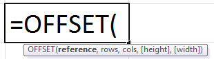
The function accepts the following mandatory arguments:
- Reference: This is the starting point from which the calculation of the ending cell (or range) address begins. It can be entered as a cell or a range of adjacent cells.
- Rows: This is the number of rows that the function needs to move. The movement can be either above or below the reference point (starting point). If this argument is positive, the function moves below the reference point. If this argument is negative, the function moves above the reference point.
- Cols: This is the number of columns that the function needs to move. The movement can be either to the right or the left of the reference point (starting point). If this argument is positive, the function moves to the right of the reference point. If this argument is negative, the function moves to the left of the reference point.
The function accepts the following optional arguments:
- Height: This is the height (number of rows) of the range to be returned.
- Width: This is the width (number of columns) of the range to be returned.
The “height” and the “width” arguments should always be positive numbers. If either of these arguments is omitted, the height and width of the reference (starting point) is assumed.
Note 1: The arguments “rows” and “cols” are specified using the reference point as the base.
Note 2: If both the “height” and “width” arguments are 1, the OFFSET excel function returns the value of a cell. This is because a 1-row by 1-column range is the dimension (size) of a single cell.
Note 3: The OFFSET function does not move any cell or range. It just returns the value of the cell (or range) address that it calculates.
How to use the OFFSET Function in Excel?
The OFFSET function is a built-in function of Excel. Let us understand its working with the help of a few examples.
Every example covers a different case of the OFFSET excel function, including an explanation of the same. In the last two examples (example #4 and #5), the OFFSET function has been combined with the arithmetic functions.
You can download this OFFSET Function Excel Template here – OFFSET Function Excel Template
Example #1–End Point is a Data Cell
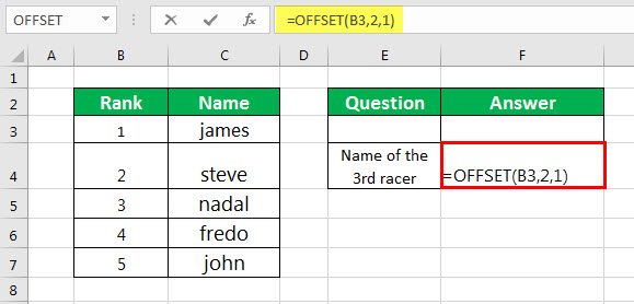
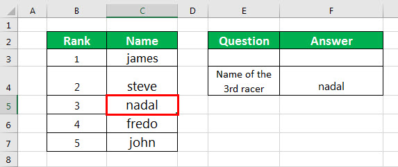
The following table shows the names of five racers and the corresponding ranks obtained by them. We want to find the name of the third racer with the help of the OFFSET function.
Step 1: Enter the following OFFSET formula in cell F4.
“=OFFSET(B3,2,1)”
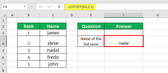
Step 2: Press the “Enter” key. The output appears in cell F4. Hence, “Nadal” is the racer who ranked third in the race.
Explanation: The first argument of the OFFSET excel function is cell B3, which is the reference point (starting point).
The “rows” argument is 2. So, the function moves two rows below cell B3, which is the cell B5. The “cols” argument is 1. So, the function moves one column to the right of cell B3, which is the cell C5.
The value of the resulting cell (end point) C5 is “Nadal.” Hence, the output in cell F4 is “Nadal.” The end point is shown in the following image.
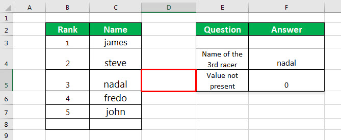
Example #2–End Point is an Empty Cell
Working on the data of example #1, we want the OFFSET function to return the value of the empty cell D5.
Step 1: Enter the following formula in cell F5.
“=OFFSET(B3,2,2)”

Step 2: Press the “Enter” key. The output 0 appears in cell F5. Hence, the OFFSET function returns the value of an empty cell as zero.

Explanation: In the given OFFSET excel formula, the reference point (starting point) is cell B3.
Since the “rows” argument is 2, the function moves two rows down to cell B5. The “cols” argument is also 2. So, the function moves two columns to the right of cell B3, which is the cell D5.
The resulting cell (end point) is D5. Since this cell is empty, the output returned by the OFFSET function is 0. The end point is shown in the following image.
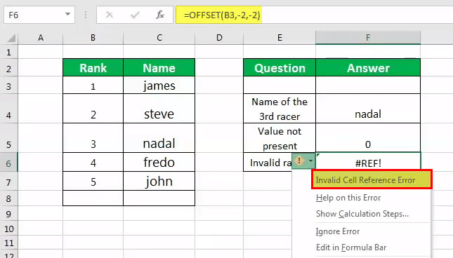
Example #3–End Point is a Non-existent Cell
Working on the data of example #1, we want the OFFSET function to return the value of a cell (to the immediate left of cell A1) that does not exist.
Step 1: Enter the following OFFSET excel formula in cell F6.
“=OFFSET(B3,-2,-2)”

Step 2: Press the “Enter” key. The output appears in cell F6. Hence, the value of a non-existent cell is a “#REF!” error.

Explanation: In this example, cell B3 is the reference point.
The “rows” argument is -2. So, the function moves two rows above the cell B3, which is the cell B1. The “cols” argument is also -2. So, the function moves two columns to the left of cell B3. However, there is no column to the left of column A.
Hence, there is no resulting cell (end point). So, the output is “#REF!” error, as shown in the following image. The icon in yellow shows “invalid cell reference error.”
Note: If the end point of the OFFSET function is a cell which is out-of-range or non-existent, it returns a “#REF” error.
Example #4–Sum of Values of the Returned Range Address
The following table shows five stocks with their maximum and minimum returns (in $). We want to sum the maximum returns of these stocks. Use the OFFSET excel function combined with the SUM functionThe SUM function in excel adds the numerical values in a range of cells. Being categorized under the Math and Trigonometry function, it is entered by typing “=SUM” followed by the values to be summed. The values supplied to the function can be numbers, cell references or ranges.read more.
Step 1: Enter the following formula in cell F3.
“=SUM(OFFSET(C2,0,0,5,1))”

Step 2: Press the “Enter” key. The output appears in cell F3. Hence, the sum of the maximum returns of the given stocks is $449.
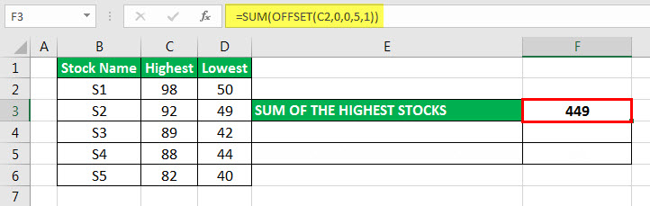
Explanation: The cell C2 is the reference point.
Both the arguments “rows” and “columns” are zero. This implies that the OFFSET function will neither move up and down nor to the left and right.
The “height” argument is 5, implying that the OFFSET function will sum five rows beginning from the cell C2. This is the range C2:C6.
The “width” argument is 1, implying that the OFFSET function will sum the values of one column (column C).
With the given “height” and “width” arguments, the preceding formula (entered in step 1) returns the sum of values of a 5-row by 1-column range. It sums the values of the returned range (5-row by 1-column) because the OFFSET is enclosed within the SUM function.
Hence, the sum of all values of column C is calculated as 98+92+89+88+82=449.
Example #5–Average of Values of the Returned Range Address
Working on the data of example #4, we want to calculate the average returns of stock “S1.” Use the OFFSET excle function combined with the AVERAGE functionThe AVERAGE function in Excel gives the arithmetic mean of the supplied set of numeric values. This formula is categorized as a Statistical Function. The average formula is =AVERAGE(read more.
Step 1: Enter the following formula in cell F5.
“=AVERAGE(OFFSET(C2,0,0,1,2))”
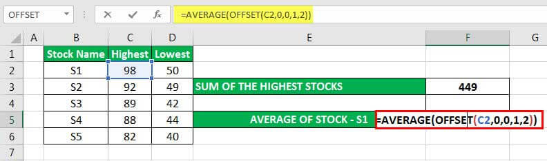
Step 2: Press the “Enter” key. The output appears in cell F5. Hence, the average return of stock “S1” is $74.
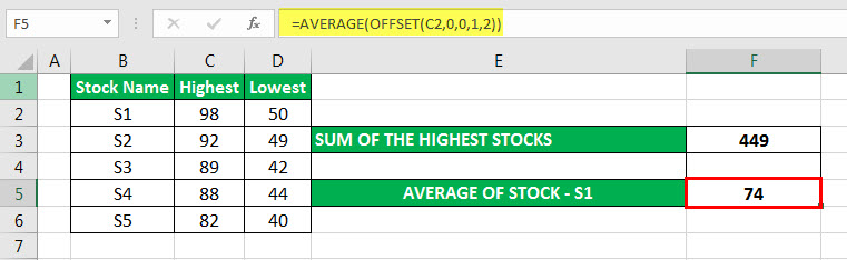
Explanation: The cell C2 is the reference point.
Both the arguments “rows” and “columns” are zero. This implies that the OFFSET function will not move in any direction.
The “height” argument is 1. This implies that the OFFSET function will consider only one row (row 2) for calculating the average.
The “width” argument is 2. This implies that the OFFSET excel function will calculate the average of two columns (columns C and D).
With the given “height” and “width” arguments, the preceding formula (entered in step 1) returns the average of a 1-row by 2-column range.
In the preceding formula, the OFFSET is enclosed within the AVERAGE function. So, the values of the returned range (1-row by 2-column) are used for calculating the average. Hence, the average of the values in the cells C2 and D2 is calculated as (98+50)/2=74.
Range Returned by the OFFSET Excel Function
The OFFSET function can also return the values of a range of adjacent cells. For this, the steps to be performed are listed as follows:
- Select a blank range of the size which is the same as specified by the “height” and “width” arguments of the OFFSET function in excel.
- Insert the OFFSET formula in the leftmost, top cell of the blank range.
- Press “Ctrl+Shift+Enter.” The curly brackets appear at the beginning and the end of the formula.
The values of the range of cells are obtained as the output of the OFFSET excel function.
Note: To obtain the values of a range of cells, it is essential to supply the “height” (number of rows) and “width” (number of columns) arguments.
Frequently Asked Questions
1. Define the OFFSET function of Excel.
The OFFSET function in excel returns the value of a single cell or a range of adjacent cells. The address of this cell (or range) is calculated from a reference point (starting cell) supplied as an argument. This reference point is taken as the base for specifying the “rows” and “cols” arguments.
The syntax of the OFFSET excel function is stated as follows:
“=OFFSET(reference,rows,cols,[height],[width])”
The OFFSET function accepts the following arguments:
Reference: This is the starting point or the base from which the calculation of the cell (or range) address begins. It can be either a single cell or a range of adjacent cells.
Rows: This is the number of rows the function needs to move. It is calculated from the starting point. A positive number implies a downward movement, while a negative number implies an upward movement.
Cols: This is the number of columns the function needs to move. This is also calculated from the starting point. A positive number implies a rightward movement, while a negative number implies a leftward movement.
Height: This is the height (number of rows) of the range that is to be returned.
Width: This is the width (number of columns) of the range that is to be returned.
The first three arguments are mandatory, while the last two are optional.
Note: To obtain the values of a range of cells, select a blank range of the same height and width as specified in the argument. Next, insert the OFFSET formula and press “Ctrl+Shift+Enter.”
2. What is the SUM OFFSET formula in Excel?
In the SUM OFFSET formula, the OFFSET is enclosed within the SUM function in the following way:
“=SUM(first cell:(OFFSET(cell containing total,-1,0)))”
The “first cell” is the first cell address whose value is to be added. The “cell containing total” is the output cell (containing the total) at the end of the numerical cells. The numbers -1 and 0 are the “rows” and “columns” arguments respectively.
The given formula helps in finding the sum of a range of adjacent cells. The OFFSET function calculates the address of the range. The SUM function sums the values of the range.
For example, let us sum the values of column B consisting of the values 20, 35, 42, and 11 in the range B1:B4. The steps are listed as follows:
• Enter the following formula in cell B5.
“=SUM(B1:(OFFSET(B5,-1,0)))”
• Press the “Enter” key.
The output in cell B5 is 108.
3. Why should the OFFSET function be used and when should it be used in Excel?
The reasons for using the OFFSET function are listed as follows:
• It helps find the value of a cell (or range) whose address is unknown, but the starting point is known.
• It works with data in which rows or columns are added regularly.
• It helps create a dynamic range for PivotTables and PivotCharts.
• It can be combined with other functions which require the cell address to work.
The OFFSET excel function is used in the following situations:
• To include the value of a newly inserted cell in the total of a range, the OFFSET is used with the SUM function.
• To find the mean, maximum, or minimum by including the additions or deletions of rows, the OFFSET is used with the AVERAGE, MAX, and MIN functions.
• To create a dynamic drop-down list (updates with the changes in the source list), the OFFSET is used with the COUNTA function.
• To overcome the limitations of the VLOOKUP (cannot look at the left) and HLOOKUP (cannot look upwards), the OFFSET is used with the MATCH function.
Recommended Articles
This has been a guide to OFFSET function in Excel. Here we discuss how to use the OFFSET excel formula along with step by step examples. You may also look at these useful functions of Excel–
- OFFSET in VBAVBA OFFSET function facilitates the user to move down or return to a particular cell at a specific range, i.e., at a distance of a certain number of rows and columns from the current cell.read more
- FIND Function in ExcelFind function in excel finds the location of a character or a substring in a text string. In other words it finds the occurrence of a text in another text, as it gives us the position, the output returned by this function is an integer.read more
- Bubble Chart in ExcelIn Excel, a bubble chart is a type of scatter plot that uses bubbles to display values and comparisons. Like scatter plots, bubble charts compare data on both horizontal and vertical axes.read more
- Tally Chart in ExcelA tally chart is one of the techniques for collecting valuable data through tally marks from the data set. Tally marks are numbers, occurrences, or total frequencies measured for a category from the grouped observations.read more
How to Use the OFFSET Function in Excel
– 3 Examples (2023)
The OFFSET function returns a range of cells that is located a specified number of rows/columns away from a specific cell.
While this has no use on its own, it’s extremely useful in specific scenarios when combined with other functions.
The OFFSET function can be hard to understand without visualizing it, so let’s just dive in💡
To follow along with this guide, I suggest you download my sample file here.
Step 1: The reference argument
Have a quick look at the OFFSET example in the picture below.

I want you to return the salary of the person 2 rows below Abigail. So, 2 rows below row #2 in column C. And put it in E2.
Let’s get started👍
The syntax of the OFFSET function consists of 5 arguments, and 2 of them are optional.
The first part of the syntax is the reference argument.
The reference argument is the starting cell from where you want to go X rows down/up or Y columns right/left.
Write:
=OFFSET(C2

So, to go 2 rows down from Abigail’s salary, you need to start in C2.
And as always, end the argument with a comma to let the OFFSET function know you’re moving to the next part of its syntax.
Step 2: The rows argument
The rows argument tells the OFFSET function the vertical location of the range you want to return (down/up)
You want to return something 2 rows below the starting reference.
So, write 2.

The rows argument works with both positive numbers and negative numbers.
– (minus) is up
+ (plus) is down
So, if you wanted to return something 1 row above the starting reference, you would write -2 instead.
Your OFFSET function should look like this by now:
=OFFSET(C2,2
Almost done already⏱️
Step 3: The columns argument
The columns argument tells the OFFSET function the horizontal location of the range you want to return.
In this example, the cell you want to return is located in the same column as the starting reference.
So, you actually don’t want to tell the OFFSET function to go any columns to the left or right.
But you do need to tell OFFSET that you want to stay in the same column.
So, write 0.

Your OFFSET function should look like this:
=OFFSET(C2,2,0
Now, if you wanted to return something that’s not in the same column as the starting reference you could write a positive or negative number instead.
– (negative) is left
+ (positive) is right
So, if you wanted to return the ‘Division’ from column B instead, you’d have to write -1.

Write and end parenthesis to close the function.
So the final function should look like this, for returning the salary 2 rows below Abigail’s (no column change).
=OFFSET(c2,2,0)

And that’s exactly what it does.
The OFFSET function returns the contents of the cell 2 cells below the starting cell.
Beautiful, right?
“But Kasper… What about the other 2 arguments?
They’re optional😊
Let me explain…
Step 4: Height and width arguments (optional)
The height and width arguments are only used to return a range of multiple adjacent cells.
In the above example, where you wanted to return the content of a single cell, the height and width arguments are useless.
For returning a range, the height and width arguments are for determining the size of that range.
Height = number of rows
Width = number of columns
The top left part of the range, is the ending point after the first 3 arguments.
And as earlier:
– (negative) is left
+ (positive) is right
Here are two OFFSET function examples that focus entirely on the height and width arguments:

The left OFFSET example
=OFFSET(A1,1,2,2,-2)
It starts in cell A1, then goes 1 row down and 3 columns to the right. We’ll call this point B.
From there it starts selecting a range that is 2 rows high (going down from the top of point B) and 2 columns wide (going left of B).
The right OFFSET example
=OFFSET(A1,2,3,1,-2)
It starts in cell A1, then goes 2 rows down and 3 columns to the right. We’ll call this point B.
From there it starts selecting a range that is 1 row high (going down from the top of point B) and 2 columns wide (going left of B).
“How’s that useful?”
That’s a good question.
On its own, it isn’t🤷
But you can use the offset function to return a range of cells into another function – and that’s where the magic starts.
Example: OFFSET dynamic range (COUNTA)
A dynamic range is a range that automatically expands to the amount of data within it.
When you combine the OFFSET function with the COUNTA function, you create a dynamic range.
This is especially useful when combined with a ‘named range’ to make a ‘dynamic named range’.
Let’s dive in🤿
Understanding dynamic named ranges
The normal syntax for the OFFSET function is:
=OFFSET(reference, rows, columns, [height], [width])
Replace the height argument and the width argument with the COUNTA function. Like this:
=OFFSET(reference, rows, columns, COUNTA(range), COUNTA(range))
As you can see, the 1st COUNTA function replaces the height argument, and the 2nd COUNTA function replaces the width argument.
But typically, you don’t need ranges wider than 1 column in dynamic named ranges.
So, this is the syntax you need to use:
=OFFSET(reference, rows, columns, COUNTA(range))
Step 1: Set starting reference
To start this OFFSET formula, make a cell reference to where the dynamic range should start:
=OFFSET($A$2

IMPORTANT:
Do remember to lock all references used in this OFFSET formula🔒
Step 2: Set rows and columns arguments to 0
Add 0 for the number of rows and columns.
=OFFSET($A$2,0,0
Step 3: Replace height argument with COUNTA function
Add the COUNTA function instead of the normal height argument.
=OFFSET(A$2$,0,0,COUNTA($A:$A))

This tells the OFFSET formula how tall the range should be to match the data in it.
It does so by counting the number of non-empty cells in the specified range using the COUNTA function. The count is returned to the OFFSET function as the height argument – the number of rows the range should include.
Step 4: Open Name Manager
Open the ‘Name Manager’ from the Formulas tab.

Step 5: Create a new named range
Click the ‘New’ button to create a new named range.

Step 6: Insert OFFSET formula
Copy the OFFSET formula you made before into the ‘Refers to’ field.

Click OK and close the Name Manager.
That’s it👏
Now, you can use your new dynamic named range in your Excel formulas.

A ‘dynamic named range’ is great for keeping your ranges tight, so they don’t include any empty cells that slow down your file.
But the ‘dynamic named range’ truly shines when used as the source in a drop-down list☀️
Example: OFFSET and MATCH function
The combination of OFFSET and MATCH is a lookup formula just like VLOOKUP or INDEX MATCH.
Especially like INDEX MATCH!
MATCH looks for a value and returns the row number of the found value to the OFFSET function. And the OFFSET function returns the cell content of a corresponding cell in the same row as the found value.
The syntax of the normal OFFSET function looks like this:
=OFFSET(starting cell, rows, columns, [height], [width])
We’re not using the last 2 arguments here, so we’ll use this and then insert the MATCH function later:
=OFFSET(starting cell, rows, columns)
Let’s look up a name and return that person’s salary.

Step 1: Set the starting cell reference
Start writing the OFFSET formula:
=OFFSET(A1,

Step 2: Replace rows argument with MATCH function
The 2nd argument of the OFFSET function determines how much down/up it should return something from. Instead of writing a value here, use the MATCH function to find it automatically.
=OFFSET(A1,MATCH(
Step 3: MATCH lookup value
You use the MATCH function as you normally would. So, start with making a cell reference to the value you want to look for (the lookup value).
=OFFSET(A1,MATCH(E2,

Step 4: MATCH lookup array
The lookup array is the column where you want to search for the lookup value.
When lookup for a name, it’s the “Name” column (column A).
=OFFSET(A1,MATCH(E2,A2:A100,

Step 5: MATCH type
The last argument of the MATCH function determines which type of match you want.
99% of the time, you want an exact match. So, write:
=OFFSET(A1,MATCH(E2,A2:A100,0),

Step 6: OFFSET function columns argument
The MATCH function found the lookup value and knows which row it is located in. It returns that row number to the OFFSET function.
But the last part of the OFFSET function determines which column, in the same row as the lookup value, to return the cell content from.

The “return column” is located 2 columns to the right of the starting cell (the first argument of the OFFSET function, A1).
Your final OFFSET formula should look like this:
=OFFSET(A1,MATCH(E2,A2:A100,0),2)
And that returns the salary for Samuel. Yay🎉

That’s it – What’s next?
That was how to use the OFFSET function in Excel – aaaaand a whole lot more😉
Like how to make dynamic ranges with OFFSET, how to use OFFSET from the current cell, and how to combine the OFFSET function and the MATCH function.
Although it is very handy – returning ranges with the OFFSET function is a very niche part of Microsoft Excel. It’s not something you need to use all the time.
However, there are other functions you actually do need all the time, like SUMIF, IF, and VLOOKUP.
Please, click here to sign up for my free 30-minute email course that teaches you these functions (and more!).
Other resources
OFFSET is a very unique function that’s almost only useful when combined with other Excel functions.
If you want to take it a step further with niche functions like OFFSET, I suggest you take a look at the INDEX function and INDIRECT function.
Frequently asked questions
Got any specific questions about the OFFSET function?
Read below and you may find your answer😊
The OFFSET function returns a range into another function. You determine the location and the size of that range by using the arguments of the OFFSET function syntax. The OFFSET function doesn’t work great on its own and should be combined with other functions.
=OFFSET(A1,2,3)
This OFFSET formula returns what’s in the cell 3 columns right and 2 rows down from cell A1. This can be used in combination with other functions such as COUNTA to make a dynamic range or MATCH to make a lookup formula.
Use this Excel formula to offset X rows and Y columns from the current cell (the cell that contains the formula):
=OFFSET(INDIRECT(ADDRESS(ROW(),COLUMN(),4)),X,Y)
Replace X and Y with numbers that indicate the location of the cell you want to return.
Kasper Langmann2023-02-23T15:06:14+00:00
Page load link