The monte carlo simulation in excel - Word и Excel - помощь в работе с программами

Excel for Microsoft 365 Excel 2021 Excel 2019 Excel 2016 Excel 2013 Excel 2010 Excel 2007 More…Less

This article was adapted from Microsoft Excel Data Analysis and Business Modeling by Wayne L. Winston.

Who uses Monte Carlo simulation?
What happens when you type =RAND() in a cell?
How can you simulate values of a discrete random variable?
How can you simulate values of a normal random variable?
How can a greeting card company determine how many cards to produce?

We would like to accurately estimate the probabilities of uncertain events. For example, what is the probability that a new product’s cash flows will have a positive net present value (NPV)? What is the risk factor of our investment portfolio? Monte Carlo simulation enables us to model situations that present uncertainty and then play them out on a computer thousands of times.

Note: The name Monte Carlo simulation comes from the computer simulations performed during the 1930s and 1940s to estimate the probability that the chain reaction needed for an atom bomb to detonate would work successfully. The physicists involved in this work were big fans of gambling, so they gave the simulations the code name Monte Carlo.

In the next five chapters, you will see examples of how you can use Excel to perform Monte Carlo simulations.

Many companies use Monte Carlo simulation as an important part of their decision-making process. Here are some examples.

General Motors, Proctor and Gamble, Pfizer, Bristol-Myers Squibb, and Eli Lilly use simulation to estimate both the average return and the risk factor of new products. At GM, this information is used by the CEO to determine which products come to market.
GM uses simulation for activities such as forecasting net income for the corporation, predicting structural and purchasing costs, and determining its susceptibility to different kinds of risk (such as interest rate changes and exchange rate fluctuations).
Lilly uses simulation to determine the optimal plant capacity for each drug.
Proctor and Gamble uses simulation to model and optimally hedge foreign exchange risk.
Sears uses simulation to determine how many units of each product line should be ordered from suppliers—for example, the number of pairs of Dockers trousers that should be ordered this year.
Oil and drug companies use simulation to value «real options,» such as the value of an option to expand, contract, or postpone a project.
Financial planners use Monte Carlo simulation to determine optimal investment strategies for their clients’ retirement.

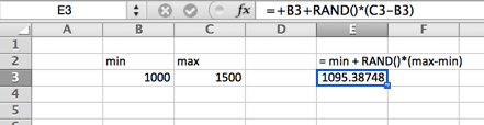
When you type the formula =RAND() in a cell, you get a number that is equally likely to assume any value between 0 and 1. Thus, around 25 percent of the time, you should get a number less than or equal to 0.25; around 10 percent of the time you should get a number that is at least 0.90, and so on. To demonstrate how the RAND function works, take a look at the file Randdemo.xlsx, shown in Figure 60-1.

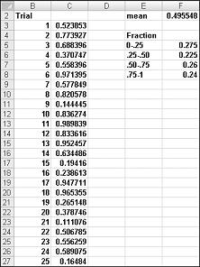
Note: When you open the file Randdemo.xlsx, you will not see the same random numbers shown in Figure 60-1. The RAND function always automatically recalculates the numbers it generates when a worksheet is opened or when new information is entered into the worksheet.

First, copy from cell C3 to C4:C402 the formula =RAND(). Then you name the range C3:C402 Data. Then, in column F, you can track the average of the 400 random numbers (cell F2) and use the COUNTIF function to determine the fractions that are between 0 and 0.25, 0.25 and 0.50, 0.50 and 0.75, and 0.75 and 1. When you press the F9 key, the random numbers are recalculated. Notice that the average of the 400 numbers is always approximately 0.5, and that around 25 percent of the results are in intervals of 0.25. These results are consistent with the definition of a random number. Also note that the values generated by RAND in different cells are independent. For example, if the random number generated in cell C3 is a large number (for example, 0.99), it tells us nothing about the values of the other random numbers generated.

Suppose the demand for a calendar is governed by the following discrete random variable:

Demand	Probability
10,000	0.10
20,000	0.35
40,000	0.3
60,000	0.25

How can we have Excel play out, or simulate, this demand for calendars many times? The trick is to associate each possible value of the RAND function with a possible demand for calendars. The following assignment ensures that a demand of 10,000 will occur 10 percent of the time, and so on.

Demand	Random number assigned
10,000	Less than 0.10
20,000	Greater than or equal to 0.10, and less than 0.45
40,000	Greater than or equal to 0.45, and less than 0.75
60,000	Greater than or equal to 0.75

To demonstrate the simulation of demand, look at the file Discretesim.xlsx, shown in Figure 60-2 on the next page.

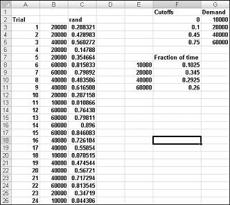
The key to our simulation is to use a random number to initiate a lookup from the table range F2:G5 (named lookup). Random numbers greater than or equal to 0 and less than 0.10 will yield a demand of 10,000; random numbers greater than or equal to 0.10 and less than 0.45 will yield a demand of 20,000; random numbers greater than or equal to 0.45 and less than 0.75 will yield a demand of 40,000; and random numbers greater than or equal to 0.75 will yield a demand of 60,000. You generate 400 random numbers by copying from C3 to C4:C402 the formula RAND(). You then generate 400 trials, or iterations, of calendar demand by copying from B3 to B4:B402 the formula VLOOKUP(C3,lookup,2). This formula ensures that any random number less than 0.10 generates a demand of 10,000, any random number between 0.10 and 0.45 generates a demand of 20,000, and so on. In the cell range F8:F11, use the COUNTIF function to determine the fraction of our 400 iterations yielding each demand. When we press F9 to recalculate the random numbers, the simulated probabilities are close to our assumed demand probabilities.

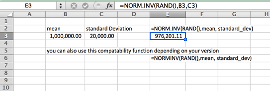
If you type in any cell the formula NORMINV(rand(),mu,sigma), you will generate a simulated value of a normal random variable having a mean mu and standard deviation sigma. This procedure is illustrated in the file Normalsim.xlsx, shown in Figure 60-3.

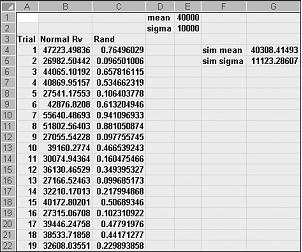
Let’s suppose we want to simulate 400 trials, or iterations, for a normal random variable with a mean of 40,000 and a standard deviation of 10,000. (You can type these values in cells E1 and E2, and name these cells mean and sigma, respectively.) Copying the formula =RAND() from C4 to C5:C403 generates 400 different random numbers. Copying from B4 to B5:B403 the formula NORMINV(C4,mean,sigma) generates 400 different trial values from a normal random variable with a mean of 40,000 and a standard deviation of 10,000. When we press the F9 key to recalculate the random numbers, the mean remains close to 40,000 and the standard deviation close to 10,000.

Essentially, for a random number x, the formula NORMINV(p,mu,sigma) generates the pth percentile of a normal random variable with a mean mu and a standard deviation sigma. For example, the random number 0.77 in cell C4 (see Figure 60-3) generates in cell B4 approximately the 77th percentile of a normal random variable with a mean of 40,000 and a standard deviation of 10,000.

In this section, you will see how Monte Carlo simulation can be used as a decision-making tool. Suppose that the demand for a Valentine’s Day card is governed by the following discrete random variable:

Demand	Probability
10,000	0.10
20,000	0.35
40,000	0.3
60,000	0.25

The greeting card sells for $4.00, and the variable cost of producing each card is $1.50. Leftover cards must be disposed of at a cost of $0.20 per card. How many cards should be printed?

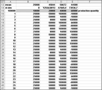
Basically, we simulate each possible production quantity (10,000, 20,000, 40,000, or 60,000) many times (for example, 1000 iterations). Then we determine which order quantity yields the maximum average profit over the 1000 iterations. You can find the data for this section in the file Valentine.xlsx, shown in Figure 60-4. You assign the range names in cells B1:B11 to cells C1:C11. The cell range G3:H6 is assigned the name lookup. Our sales price and cost parameters are entered in cells C4:C6.

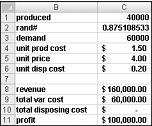
You can enter a trial production quantity (40,000 in this example) in cell C1. Next, create a random number in cell C2 with the formula =RAND(). As previously described, you simulate demand for the card in cell C3 with the formula VLOOKUP(rand,lookup,2). (In the VLOOKUP formula, rand is the cell name assigned to cell C3, not the RAND function.)

The number of units sold is the smaller of our production quantity and demand. In cell C8, you compute our revenue with the formula MIN(produced,demand)*unit_price. In cell C9, you compute total production cost with the formula produced*unit_prod_cost.

If we produce more cards than are in demand, the number of units left over equals production minus demand; otherwise no units are left over. We compute our disposal cost in cell C10 with the formula unit_disp_cost*IF(produced>demand,produced–demand,0). Finally, in cell C11, we compute our profit as revenue– total_var_cost-total_disposing_cost.

We would like an efficient way to press F9 many times (for example, 1000) for each production quantity and tally our expected profit for each quantity. This situation is one in which a two-way data table comes to our rescue. (See Chapter 15, «Sensitivity Analysis with Data Tables,» for details about data tables.) The data table used in this example is shown in Figure 60-5.

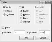
In the cell range A16:A1015, enter the numbers 1–1000 (corresponding to our 1000 trials). One easy way to create these values is to start by entering 1 in cell A16. Select the cell, and then on the Home tab in the Editing group, click Fill, and select Series to display the Series dialog box. In the Series dialog box, shown in Figure 60-6, enter a Step Value of 1 and a Stop Value of 1000. In the Series In area, select the Columns option, and then click OK. The numbers 1–1000 will be entered in column A starting in cell A16.

Next we enter our possible production quantities (10,000, 20,000, 40,000, 60,000) in cells B15:E15. We want to calculate profit for each trial number (1 through 1000) and each production quantity. We refer to the formula for profit (calculated in cell C11) in the upper-left cell of our data table (A15) by entering =C11.

We are now ready to trick Excel into simulating 1000 iterations of demand for each production quantity. Select the table range (A15:E1014), and then in the Data Tools group on the Data tab, click What If Analysis, and then select Data Table. To set up a two-way data table, choose our production quantity (cell C1) as the Row Input Cell and select any blank cell (we chose cell I14) as the Column Input Cell. After clicking OK, Excel simulates 1000 demand values for each order quantity.

To understand why this works, consider the values placed by the data table in the cell range C16:C1015. For each of these cells, Excel will use a value of 20,000 in cell C1. In C16, the column input cell value of 1 is placed in a blank cell and the random number in cell C2 recalculates. The corresponding profit is then recorded in cell C16. Then the column cell input value of 2 is placed in a blank cell, and the random number in C2 again recalculates. The corresponding profit is entered in cell C17.

By copying from cell B13 to C13:E13 the formula AVERAGE(B16:B1015), we compute average simulated profit for each production quantity. By copying from cell B14 to C14:E14 the formula STDEV(B16:B1015), we compute the standard deviation of our simulated profits for each order quantity. Each time we press F9, 1000 iterations of demand are simulated for each order quantity. Producing 40,000 cards always yields the largest expected profit. Therefore, it appears that producing 40,000 cards is the proper decision.

The Impact of Risk on Our Decision If we produced 20,000 instead of 40,000 cards, our expected profit drops approximately 22 percent, but our risk (as measured by the standard deviation of profit) drops almost 73 percent. Therefore, if we are extremely averse to risk, producing 20,000 cards might be the right decision. Incidentally, producing 10,000 cards always has a standard deviation of 0 cards because if we produce 10,000 cards, we will always sell all of them without any leftovers.

Note: In this workbook, the Calculation option is set to Automatic Except For Tables. (Use the Calculation command in the Calculation group on the Formulas tab.) This setting ensures that our data table will not recalculate unless we press F9, which is a good idea because a large data table will slow down your work if it recalculates every time you type something into your worksheet. Note that in this example, whenever you press F9, the mean profit will change. This happens because each time you press F9, a different sequence of 1000 random numbers is used to generate demands for each order quantity.

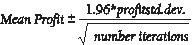
Confidence Interval for Mean Profit A natural question to ask in this situation is, into what interval are we 95 percent sure the true mean profit will fall? This interval is called the 95 percent confidence interval for mean profit. A 95 percent confidence interval for the mean of any simulation output is computed by the following formula:

In cell J11, you compute the lower limit for the 95 percent confidence interval on mean profit when 40,000 calendars are produced with the formula D13–1.96*D14/SQRT(1000). In cell J12, you compute the upper limit for our 95 percent confidence interval with the formula D13+1.96*D14/SQRT(1000). These calculations are shown in Figure 60-7.

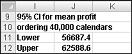
We are 95 percent sure that our mean profit when 40,000 calendars are ordered is between $56,687 and $62,589.

A GMC dealer believes that demand for 2005 Envoys will be normally distributed with a mean of 200 and standard deviation of 30. His cost of receiving an Envoy is $25,000, and he sells an Envoy for $40,000. Half of all the Envoys not sold at full price can be sold for $30,000. He is considering ordering 200, 220, 240, 260, 280, or 300 Envoys. How many should he order?

A small supermarket is trying to determine how many copies of People magazine they should order each week. They believe their demand for People is governed by the following discrete random variable:

Demand	Probability
15	0.10
20	0.20
25	0.30
30	0.25
35	0.15

The supermarket pays $1.00 for each copy of People and sells it for $1.95. Each unsold copy can be returned for $0.50. How many copies of People should the store order?

Need more help?

You can always ask an expert in the Excel Tech Community or get support in the Answers community.

Need more help?

Источник

A Monte Carlo simulation can be developed using Microsoft Excel and a game of dice. A Monte Carlo simulation is a method for modeling probabilities by using random numbers to approximate and simulate possible outcomes. Today, it is widely used as an analysis tool. It plays a key part in various fields such as finance, physics, chemistry, and economics.

Key Takeaways

The Monte Carlo method seeks to improve the analysis of data using random data sets and probability calculations.
A Monte Carlo simulation can be developed using Microsoft Excel and a game of dice.
A data table can be used to generate the results—a total of5,000 results are needed to prepare the Monte Carlo simulation.

Monte Carlo Simulation

The Monte Carlo method was invented by John von Neumann and Stanislaw Ulam in the 1940s and seeks to solve complex problems using random and probabilistic methods. The term Monte Carlo refers the administrative area of Monaco popularly known as a place where European elites gamble.

The Monte Carlo simulation method computes the probabilities for integrals and solves partial differential equations, thereby introducing a statistical approach to risk in a probabilistic decision. Although many advanced statistical tools exist to create Monte Carlo simulations, it is easier to simulate the normal law and the uniform law using Microsoft Excel and bypass the mathematical underpinnings.

When to Use the Monte Carlo Simulation

We use the Monte Carlo method when a problem is too complex and difficult to do by direct calculation. Using the simulation can help provide solutions for situations that prove uncertain. A large number of iterations allows a simulation of the normal distribution. It can also be used to understand how risk works, and to comprehend the uncertainty in forecasting models.

As noted above, the simulation is often used in many different disciplines including finance, science, engineering, and supply chain management—especially in cases where there are far too many random variables in play. For example, analysts may use Monte Carlo simulations in order to evaluate derivatives including options or to determine risks including the likelihood that a company may default on its debts.

Game of Dice

For the Monte Carlo simulation, we isolate a number of key variables that control and describe the outcome of the experiment, then assign a probability distribution after a large number of random samples is performed. In order to demonstrate, let’s take a game of dice as a model. Here’s how the dice game rolls:

• The player throws three dice that have six sides three times.

• If the total of the three throws is seven or 11, the player wins.

• If the total of the three throws is: three, four, five, 16, 17, or 18, the player loses.

• If the total is any other outcome, the player plays again and re-rolls the dice.

• When the player throws the dice again, the game continues in the same way, except that the player wins when the total is equal to the sum determined in the first round.

It is also recommended to use a data table to generate the results. Moreover, 5,000 results are needed to prepare the Monte Carlo simulation.

To prepare the Monte Carlo simulation, you need 5,000 results.

Step 1: Dice Rolling Events

First, we develop a range of data with the results of each of the three dice for 50 rolls. To do this, it is proposed to use the «RANDBETWEEN(1,6)» function. Thus, each time we click F9, we generate a new set of roll results. The «Outcome» cell is the sum total of the results from the three rolls.

Step 2: Range of Outcomes

Then, we need to develop a range of data to identify the possible outcomes for the first round and subsequent rounds. There is a three-column data range. In the first column, we have the numbers one to 18. These figures represent the possible outcomes following rolling the dice three times: The maximum being 3 x 6 = 18. You will note that for cells one and two, the findings are N/A since it is impossible to get a one or a two using three dice. The minimum is three.

In the second column, the possible conclusions after the first round are included. As stated in the initial statement, either the player wins (Win) or loses (Lose), or they replay (Re-roll), depending on the result (the total of three dice rolls).

In the third column, the possible conclusions to subsequent rounds are registered. We can achieve these results using the «IF» function. This ensures that if the result obtained is equivalent to the result obtained in the first round, we win, otherwise we follow the initial rules of the original play to determine whether we re-roll the dice.

Step 3: Conclusions

In this step, we identify the outcome of the 50 dice rolls. The first conclusion can be obtained with an index function. This function searches the possible results of the first round, the conclusion corresponding to the result obtained. For example, when we roll a six, we play again.

One can get the findings of other dice rolls, using an «OR» function and an index function nested in an «IF» function. This function tells Excel, «If the previous result is Win or Lose,» stop rolling the dice because once we have won or lost we are done. Otherwise, we go to the column of the following possible conclusions and we identify the conclusion of the result.

Step 4: Number of Dice Rolls

Now, we determine the number of dice rolls required before losing or winning. To do this, we can use a «COUNTIF» function, which requires Excel to count the results of «Re-roll» and add the number one to it. It adds one because we have one extra round, and we get a final result (win or lose).

Step 5: Simulation

We develop a range to track the results of different simulations. To do this, we will create three columns. In the first column, one of the figures included is 5,000. In the second column, we will look for the result after 50 dice rolls. In the third column, the title of the column, we will look for the number of dice rolls before obtaining the final status (win or lose).

Then, we will create a sensitivity analysis table by using the feature data or Table Data table (this sensitivity will be inserted in the second table and third columns). In this sensitivity analysis, the numbers of events of one to 5,000 must be inserted into cell A1 of the file. In fact, one could choose any empty cell. The idea is simply to force a recalculation each time and thus get new dice rolls (results of new simulations) without damaging the formulas in place.

Step 6: Probability

We can finally calculate the probabilities of winning and losing. We do this using the «COUNTIF» function. The formula counts the number of «win» and «lose» then divides by the total number of events, 5,000, to obtain the respective proportion of one and the other. We finally see that the probability of getting a Win outcome is 73.2% and getting a Lose outcome is therefore 26.8%.

Источник

What is Monte Carlo Simulation?

Monte Carlo Simulation is a process of using probability curves to determine the likelihood of an outcome. You may scratch your head here and say… “Hey Rick, a distribution curve has an array of values. So how exactly do I determine the likelihood of an outcome?” And better yet, how do I do that in Microsoft Excel without any special add-ins

Thought you would never ask.

This is done by running the simulation thousands of times and analyzing the distribution of the output. This is particularly important when you are analyzing the output of several distribution curves that feed into one another.

Example:

# of Units Sold may have a distribution curve
multiplied by Market price, which may have another distribution curve
minus variable wages which have another curve
etc., etc.

Once all these distributions are intermingled, the output can be quite complex. Running thousands of iterations (or simulations) of these curve may give you some insights. This is particularly useful in analyzing potential risk to a decision.

Describe Monte Carlo

When describing Monte Carlo Simulation, I often refer to the 1980’s movie War Games, where a young Mathew Broderick (before Ferris Bueller) is a hacker that uses his dial up modem to hack into the Pentagon computers and start World War 3. Kind of. He then had the Pentagon computers do many simulations of the games Tic Tac Toe to teach the computer that no one will will a nuclear war – and save the world in the process.

Thanks Ferris. You’re a hero.

Here’s a glimpse of the movie to show you big time Monte Carlo in action. I am assuming that you will overlook the politics, the awkward man hugging and of course, Dabney Coleman.

The Monte Carlo Simulation Formula

Distribution Curves

There are various distribution curves you can use to set up your Monte Carlo simulation. And these curves may be interchanged based on the variable. Microsoft doesn’t have a formula called “Do Monte Carlo Simulation” in the menu bar 🙂

Uniform Distribution

In a uniform distribution, there is equal likelihood anywhere between the minimum and a maximum. A uniform distribution looks like a rectangle.

Normal (Gaussian) Distribution

This is also your standard bell shaped curve. This Monte Carlo Simulation Formula is characterized by being evenly distributed on each side (median and mean is the same – and no skewness). The tails of the curve go on to infinity. So this may not be the ideal curve for house prices, where a few top end houses increase the average (mean) well above the median, or in instances where there is a hard minimum or maximum. An example of this may be the minimum wage in your locale. Please note that the name of the function varies depending on your version.

Lognormal Distribution

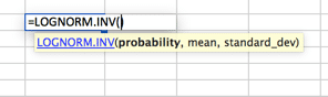
A distribution where the logarithm is normally distributed with the mean and standard deviation. So the setup is similar to the normal distribution, but please note that the mean and standard_dev variables are meant to represent the logarithm.

Poisson Distribution

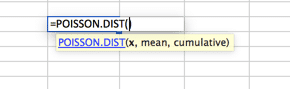
This is likely the most underutilized distribution. By default, many people use a normal distribution curve when Poisson is a better fit for their models. Poisson is best described when there is a large distribution near the very beginning that quickly dissipates to a long tail on one side. An example of this would be a call center, where no calls are answered before second ZERO. Followed by the majority of calls answered in the first 2 intervals (say 30 and 60 seconds) with a quick drop off in volume and a long tail, with very few calls answered in 20 minutes (allegedly).

The purpose here is not to show you every distribution possible in Excel, as that is outside the scope of this article. Rather to ensure that you know that there are many options available for your Monte Carlo Simulation. Do not fall into the trap of assuming that a normal distribution curve is the right fit for all your data modeling. To find more curves, to go the Statistical Functions within your Excel workbook and investigate. If you have questions, pose them in the comments section below.

Building The Model

For this set up we will assume a normal distribution and 1,000 iterations.

Input Variables

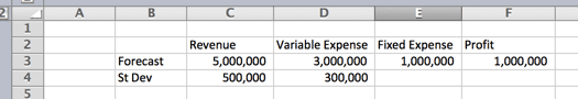
The setup assumes a normal distribution. A normal distribution requires three variables; probability, mean and standard deviation. We will tackle the mean and standard deviation in our first step. I assume a finance forecasting problem that consists of Revenue, Variable and Fixed Expenses. Where Revenue minus Variable Expenses minus Fixed Expenses equals Profit. The Fixed expenses are sunk cost in plant and equipment, so no distribution curve is assumed. Distribution curves are assumed for Revenue and Variable Expenses.

First Simulation

The example below indicates the settings for Revenue. The formula can be copy and pasted to cell D6 for variable expenses. For Revenue and expenses we you the function NORM.INV() where the parameters are:

Probability = the function RAND() to elicit a random number based on the other criteria within the distribution.
Mean = The mean used in the Step 1. For Revenue it is C3.
Standard Deviation = The Standard Deviation used in Step 1. For Revenue it is C4

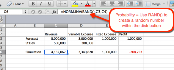
Since RAND() is used as the probability, a random probability is generated at refresh. We will use this to our advantage in the next step.

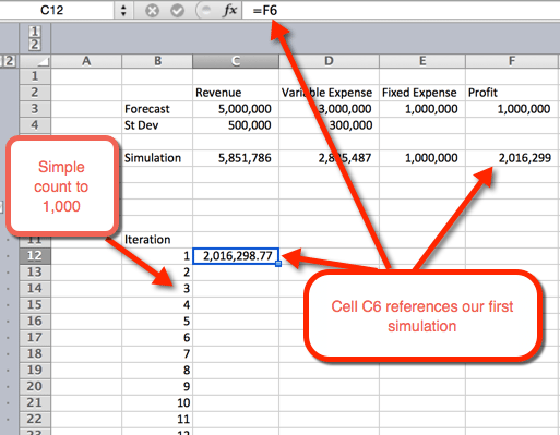
1,000 Simulations

There are several ways to do 1,000 or more variations. The simplest option is to take the formula from step #2 and make it absolute. Then copy and paste 1,000 times. That’s simple, but not very fancy. And if Ferris Bueller can save the world by showing a new Tic Tac Toe game to a computer, then we can spice up this analysis as well. Let’s venture into the world of tables.

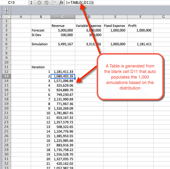
First we want to create an outline for a table. We do this by listing the numbers 1 to 1,000 in rows. In the example image below, the number list starts in B12.
in the next column, in cell C12, we will reference the first iteration.

Next highlight the area where we want to house the 1,000 iterations
Select Data > Data Tables
For Column input cell: Select a blank cell. In the download file, cell D11 is selected
Select OK

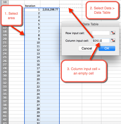
Once OK is selected from the previous step, a table is inserted that autopopulates the 1,000 simulations

Summary Statistics

Once the simulations are run, it is time to gather summary statistics. This can be done a number of ways. In this example I used the COUNTIF() function to determine the percentage of simulations that are unprofitable, and the likelihood of a profit greater than $1 Million. As expected, the likelihood of greater than $1M hovers around 50%. This is because we used normal distribution curves that are evenly distributed around the mean, which was $1M. The likelihood of losing money is 4.8%. This was gathered by using the COUNTIF() function to count the simulations that were less than zero, and dividing by the 1,000 total iterations.

Monte Carlo Simulation Formula

Get the Download

Now What?

In the video above, Oz asks about the various uses for Monte Carlo Simulation. What have you used it for? Are there any specific examples that you can share with the group? If so, leave a note below in the comments section. Also, feel free to sign up for our newsletter, so that you can stay up to date as new Excel.TV shows are announced. Leave me a message below to stay in contact.

Источник

All Time Hits, Analytics, Charts and Graphs, Excel Howtos, Featured, Huis, Learn Excel, Posts by Hui, simulation

Last updated on June 27, 2013

Chandoo

This is a Guest Post by Hui, an Excel Ninja and One of the Moderators of our Forums. Please note that this post is unusually large by Chandoo.org standards.

============================================================

If anybody asks me what is the best function in excel I am drawn between Sumproduct and Data Tables, Both make handling large amounts of data a breeze, the only thing missing is the Spandex Pants and Red Cape!

How often have you thought of or been asked “I’d like to know what our profit would be for a number of values of an input variable” or “Can I have a graph of Profit vs Cost vs …”

This post is going to detail the use of the Data Table function within Excel, which can help you answer those questions and then so so much more.

Introduction
1 Way Tables
2 Way Tables
Monitor Multiple Variables
Multiway Tables
Monte Carlo Analysis
Iterative Functions and Fractals
Download Example Workbooks

INTRODUCTION

How often have you thought “I’d like to know what our profit would be for a +/- 10, 20 and 30 % variance in the costs” ?

This post is going to detail the use of the Data Table function within Excel, which can help you answer that question.

The Data Table function is a function that allows a table of what if questions to be posed and answered simply, and is useful in simple what if questions, sensitivity analysis, variance analysis and even Monte Carlo (Stochastic) analysis of real life model within Excel.

The Data Table function should not be confused with the Insert Table function.

DATA TABLE BASICS

The Data Table function is hidden away in different locations within different versions of Excel but apart from the menu location the functionality is the same throughout.

Where is the Data Table Function

Excel 2007/10

In Excel 2007 & 2010 go to the Data Tab, What If Analysis panel and select Data Table

Excel 97-03

In Excel up to 2003 go to the Data Menu and select Table…

Both Excel 97-03 and 2007/10 then bring up the same Data Table dialog box.

… and this simple dialog box is all empowering ?

Yes !

Blue Sky Mine Co

For demonstration of the Data Table function I am going to use a simple profit model of a Gold Mine, “The Blue Sky Mine Co”. This is a fictitious mine but provides a simple model which we can use the data Table function to analyse.

It consists of 6 input variables and a simple cost and revenue model to produce a profit.

In our Blue Sky Gold Mine Co model, we can see that if we mine and treat 1,000,000 t of gold ore containing 1.68 g/t gold, we will make A$ 5.452M profit. But what if the inputs change ?

1 WAY DATA TABLES

Lets make a 1 Way Table with our Blue Sky Gold Mine Co example.

This is shown in the attached Excel Workbook on the “1 Way” Tab or 1 Way Example

In our Blue Sky Gold Mine profit calculation example, we can see that if we mine and treat 1,000,000 t of gold ore containing 1.68 g/t gold, we will make A$ 5.452M profit. But what if the grade is more or less than that value of 1.68 g/t ? After all it is only a geological estimate.

This is what the Data Table function is made for.

Next to the model add a couple of columns as shown in blue

Note: Throughout this post you will see the use of 1E6 in formulas which is simpler to write than 1,000,000.

The first column is a list of values that will be applied to each iteration of the Column Input Cell

The Top Cell of the second Column contains a formula which will retrieve the answer you want to watch, in this case Profit. It will be displayed as M$.

Now select the entire Blue Area and Select Data Table

This is the Data Table input screen.

The tricky/confusing part here is that in our example we are changing the input value to our Gold Mine Profit model using a Column of Numbers, so enter $C$6 in the Column Input Cell, Leave the Row Input Cell blank.

Click Ok

You can now see a Table of Profit Values for each Grade Value.

The variance in the Profit can easily be graphed against the Gold Grade and we can now see that if the Gold Grade is below about 1.55 g/t Au we will not make a profit and conversely if it is above 2.0 g/t Au we will make a large profit.

Before we move onto 2 Way Data Tables it is worth exploring small variations on One Way Tables.

What if my Data is in Rows?

Had our input data been arranged horizontally in Rows, we could have used a Row Input Cell to process the data.

What if I want to vary the inputs by a certain Percentage ?

Another Scenario is often where you want to vary an input by a Fixed Percentage.

This is easily done using Data Tables

Setup the input cells with the percentage variations you want to examine, noting that the values don’t have to be evenly spread.

Setup a Temporary Input Cell, This will hold the Percentage Variance briefly whilst calculations are happening. Set a default value of 0 (zero)

Change your Main Input Cell, Gold Grade in our case, to Multiply the fixed answer by 1+ the temp Input Cell.

Run the Data Table with a Column Input Cell, which will refer to the Temp Input Cell.

2 WAY DATA TABLES

So the Boss comes in and asks, what Happens if the Gold Grade changes as well as the A$/U$ Exchange Rate?

You guessed it, Two Way tables to the rescue.

This is shown in the attached Excel Workbook on the “2 Way” Tab or 2 Way Example

Two way data Tables work the same as One Way Data Tables except that you can vary 2 parameters at once.

With Two Way Data Tables you need to setup a Column of data for one Input and a Row of data for the second Input. The answer is returned at the intersection of the Row and Column.

Here we have setup a Column of Gold Grades ranging from 1.5 to 2.1 g/t Au and a Row of Exchange rates =varying from 0.70 to 1.00 A$/U$

Note at the intersection of the Row and Column there is a Reference to the variable you want to monitor in this case profit.

You can now see the variance in Profit for variations in Gold Grade and Exchange Rate.

What about varying by Percentages?

Once again we can re-arrange the input variables to examine percentage changes in the inputs via a Temporary Input Cell.

MONITORING MULTIPLE VARIABLES

So you have a complex model and want to monitor a number of input and output variables at once. No problems, Data Tables to the rescue.

In this example we are varying one input variable but monitoring 3 Output variables, 2 input variables and then doing a calculation all as part of the Data Table.

This is shown in the attached Excel Workbook on the “Monitor Multi variables” Tab or Monitor Multi Variables Example

The first 3 columns, Total Cost, Revenue and Profit are output variables even though Total Cost doesn’t change, we can still monitor it to make sure our model is working correctly

The next 2 columns, Gold Grade and Gold Price are input variables even though only Gold Grade is being varied.

The last column Cost per Oz is not calculated as part of the model (ok sometimes we forget don’t we), but it can be calculated on the fly as part of the Data Table.

The result is:

MULTIWAY DATA TABLES

But I hear you thinking, “If Data Tables are so good why can I only Change 2 variables at Once? I want to change more! “.

No Problems

Data Tables in fact allow you to Change any Number of input variables at once and monitor any number of input and output variables. It does however require a slight of hand.

This is shown in the attached Excel Workbook on the “Multi Way Tables” Tab or Multiway Table Example

First things first,

Setup a table of what scenarios you want to examine:

Setup the Data Table area to monitor Inputs, Outputs and Calculated Fields

Note that the Input Data Column will be used to select the Scenario No.

Also note that we have setup F2 to retrieve the Scenarios Name.

And in H6 we will put the Scenario name into the Data Table, who said Data Tables were only for Numbers!

Next Link the Model to the scenario

And run the Data Table

Note how the Description Column is populated with the Scenario’s Name (Text values)

So now when your boss asks you what effect the price of … has on the budget, you know where to turn.

MONTE CARLO SIMULATIONS IN EXCEL

Monte Carlo simulation (or analysis) as its name suggests puts an element of gambling into the scenarios, or more correctly allows you to measure the effect of variability on input parameters.

This is done by running scenarios against your model hundreds or thousands of times and changing the inputs each time and then measuring the effects at the end of the runs.

And Data Tables can do that? Absolutely!

First some statistics.

Everything in life has variability, from the size of Zebra’s Strips, The height of people and the Arrival times of trains, the time that people read this post, the time that it takes people to read this post.

Most things are variable around a central or mean (average) value. The spread of variability is commonly known as the distribution.

Distributions can have many names and shapes, but common ones are

Normal: Bell shaped around a mean
Uniform: All values have an even chance of selection
Exponential: Low or High values have a much higher probability that the other values

In life most distributions are Normal in nature indicating that the distribution is Bell shaped around a mean with a known method of describing the variability around this.

Excel has 2 functions that produce Random numbers, Rand() and Randbetween(). These 2 functions both have a Uniform Distribution, that is any value between the minimum and maximum values will have the same probability of being chosen.

We can convert a uniform distribution to a Normal distribution by some simple maths (simple to do, not simple to explain).

=norminv(rand(),mean,standard_dev)

Example =NORMINV(rand(),100,10)

Will generate a distribution of random numbers centred on 100 with a spread having a bell shaped curve with a standard deviation of 10. This means that the function will produce a number with a 99.7% probability of being between 70 and 130 and on average will have a mean of 100.

Monte Carlo simulations

So how can I use this and Data Tables to do Monte Carlo simulations.

Before we go any further the author wants to explicitly state that he is not suggesting that the use of Normal Distributions for the variables modeled below is appropriate, except for the purpose of demonstration of the principles behind Monte Carlo Modelling.

As with all models you need to have a good understanding of the distribution of inputs before you start playing with simulations or of which Monte Carlo is but one type. ie: Rubbish In Rubbish Out.

We can model an input vaiable, in this case Exchange rate with a distribution instead of a fixed value and then run the model a number of times and see what impact the variation has on the output.

This is shown in the attached Excel Workbook on the “Monte Carlo (Simple)” Tab or Monte Carlo (Simple) Example

The formula =NORMINV(RAND(),0.92,0.02), will generate a Random Exchange Rate with a distribution based on a mean on 0.92 A$/U$ and a spread of approximately 6 cents each way ie: there will be a 99.7% probability of the exchange rate being between 0.86 and 0.98 A$/U$.

Copying the formula down from H6 to H1005 will allow our data table to generate 1000 iterations of the model each with a randomly generated Exchange Rate.

In the model above, you can see that for a Base case exchange rate of 0.92 the profit is $M 5.452, however after running 1000 simulations the profit is actually $M 5.7134. More important is that you can now run statistics on the model to tell what is the probability of the profit being greater than 0.00 based on variance in the exchange rate etc.

Note 1: You will note that in the above data table that the Input Column (darker blue) has the formula for calculating a random input grade from a distribution. =NORMINV(RAND(),0.92,0.02)

This is a Volatile Formula , ie: It recalculates every time the worksheet changes.

What this means for the worksheet is that when the Data Table goes to Calculate Row 2 of the Data Table it will recalculate the Input value for Row 1.

On Calculation of Row 2, It doesn’t change the Table Values for Row 1, just the Input Column value.

So after 1,000 calculations of the Data Table, the Input Column values will have no relationship to the data from the original Calculations stored in the Data Table body area.

To make up for this we also add an Input variable to the Data Table.

Doing this allows the Data Table to capture and store both the Input variable and corresponding Output variable in the Data Table’s Body.

Note 2: Always run at least 1000 iterations of Monte Carlo models. This is to ensure that you have a statistical chance of getting sufficient outliers (extreme values) to make the variance analysis meaningful. This is important because as the number of iterations increases the variance of the average output decreases.

Press F9 a few times and watch the average H6:H1005 change.

Try changing the Data table from 1,000 rows to 10, 20 or 100,0000 rows. As the number of iterations increases the variance in the average of the output decreases.

Advanced Monte Carlo Simulations

We can now put our knowledge of Data Tables and Monte Carlo Simulation to the test by varying 4 input variables at the same time.

This is shown in the attached Excel Workbook on the “Monte Carlo (Advanced)” Tab or Monte Carlo (Adv) Example

In the example below we have inserted distributions for 4 input variables.

Ore Tonnes	Mean 1,000,000 tonnes	Standard Deviation of 100,000 tonnes
Gold Grade	Mean 1.68 g/t Au	Standard Deviation of 0.1 g/t Au
Gold Price	Mean 1,200 U$/Oz	Standard Deviation of 100 U$/Oz
Exchange rate	Mean 0.92 A$/U$	Standard Deviation of 0.02 A$/U$

And setup a data Table for the 4 Input Variables and main output variable, Profit.

Note: When this model is run through the Data Table, note that the Row or Column input cells can be set to anywhere. The Model is not using the value of the Input Cell (Row or Column) and isn’t even using the Run No (Column F) for the model, the data table is simply being used to run lots of iterations of the model, with the variability coming from the Random Numbers in the 4 input cells.

ITERATED FUNCTIONS INCLUDING FRACTALS

At a meeting in early 2005, the company I was working for was looking at an integrated Scheduling & Budgeting system.

The salesman gave a great demo except that the system would take approx. 30 mins to calculate our budget as opposed to a half a second in Excel.

Complaining I mentioned that our current, Excel based, system could do the job in seconds.

And he returned stating that “the system was doing a lot of things Excel couldn’t do”.

I responded “but Excel can do anything”

and he immediately shot back that “Excel can’t do a Mandelbrot”

To which I responded “Yes it can”

And he responded “Not without VB Code”

Without too much thinking I responded that I would accept the Challenge.

The attached file, which is described below is my response.

Excel Mandelbrot

The attached file is an implementation of the classic Mandelbrot implemented in Excel without the use of VBA code.

A Mandelbrot is a graphical display of the simple equation Z_n+1 = Z_n² + c, where Z is a complex number (x +iy).

Which is described at http://en.wikipedia.org/wiki/Mandelbrot_set

This can be solved in the real X-Y domain using:

Xnew = Xold² – Yold² + X_Orig and

Ynew = 2 * Yold * Xold+ Y_Orig

Study of iterated functions reveals that these functions will either converge on an answer or diverge once a boundary has been breached

In the case of the Mandelbrot, this function diverges after the function Z² > 4

So to construct a Mandelbrot a program needs simply to

Loop from Xmin to Xmax in small steps and
Loop from Ymin to Ymax in small steps and
For every X, Y Point in the above 2 loops, solve the above equations until the answer is > 4
Color the screen according to how many iterations it took to diverge or not

Simple…

Except that Excel doesn’t have any looping functions unless you use VBA Code

The calculation of the solution for any X, Y starting point is simple enough using a series of Rows and Columns where each Cells is the starting iteration of the solution for each various X, Y co-ordinate.

This is shown in the Calculations page in the Xnew, Ynew, Xold, Yold, Rsq and Count columns.

The iterations are simply done in the Xnew and Ynew columns

For each iteration we check that the Z² value hasn’t diverged (not > 4) (Xnew² + Ynew²)

And keep track of how many iterations it took to diverge, the Count Column

The above 5 lines I refer to below as the Calculator.

The trick to working out how to do this for a X-Y Grid was the use of the Table Function to send the starting positions to the Calculator and return the Count for that location.

This is the large Yellow Area.

The Large yellow area (Data Table Area) is flanked on the Top and Left by the X and Y co-ordinates for a grid encompassing the area which we want to plot.

The Table Function extracts the Top and Left values and puts them in the X Orig and Y Orig positions of the calculator.

The Calculator returns the Count of the Divergence of the Calculator to the H2 position (Top Left corner of the Grid) and that value is stored at the Grid Location.

The Data Table repeats this for each position in the X-Y Grid.

An Excel Surface Chart can then Chart the Large Yellow area in effect creating a Traditional Mandelbrot plot by joining up adjacent areas of equal value (Contouring).

The Chart can also be displayed as a 3D-Surface rather than a Contour Chart for a dramatic effect.

Zooming In can be added by adding code that allows the user to say Right click in the Large Yellow area and the code will then take the Co-ordinates and Zoom in by a fixed factor

Zooming Out can be added by adding code that allows the user to say Double click in the Large Yellow area and the code will then take the Co-ordinates and Zoom out by a fixed factor

DOWNLOAD EXAMPLE WORKBOOKS

Download the complete example workbooks described above and practice data tables on your own.

Click here to download Gold Mine Monte Carlo Simulations & Data Tables workbook. [XL 2003 version here]
Click here to download Excel Mandelbrot workbook.

Note: A few people have said the above files either Hang or Freeze there PC’s. This is probably because they have a number of large Data Tables within them.

I have uploaded each Tab as a separate Excel 2007 file, see below:

1. 1 Way.xlsx
2. 2 Way.xlsx
3. Monitor Multi Variables.xlsx
4. Multiway Table.xlsx
5. Monte Carlo Simple (updated)
6. Monte Carlo (Adv).xlsx

In the Example Files some of the Data Tables have been removed and there are instructions on how to re-instate them included in the file.

FINAL THOUGHTS

Speed

If you start adding a number of Data Tables to Complex Models you will rapidly cause even the fastest machines to grind to a halt.

VBA

The best way around the above speed issue is to setup a number of Data Tables for whatever analysis you wish to undertake. Then as you run each analysis copy the Data Table Data Area, The area between the Rows and Columns and paste it as values over itself. Then move onto the next data table and run it.

This allows the Data Tables to be quickly recalculated if required.

This process can be automated via 3 lines of VBA code for each Data Table.

‘Calculate Data Table in F5:H18, using Column Input cell C9
Range(“F5:H18”).Table ColumnInput:=Range(“C9”)

‘Copy Data Area as Values
Range(“G6:H18”).Copy
Range(“G6:H18”).PasteSpecial Paste:=xlPasteValues

‘Repeat Above for each Data Table

‘Deselect Current Range
Application.CutCopyMode = False

Cell Contents

If you look at a cell in a Data Table you will see something like:

{=TABLE(,E5)}: for a Column Input Cell
{=TABLE(E4,)}: for a Row Input Cell
{=TABLE(E4,E5)}: for a Row and Column Input Cell

Although these appear like Array Formula, they cannot be manually set.

So setting up a data table and typing =TABLE(,E5) Ctrl-Shift-Enter, only produces an error message.

Added by Chandoo

This post is by far one of the most comprehensive posts on Chandoo.org. And each of the 3100+ words in it show the passion and knowledge that Hui has. Thank you so much Hui for sharing this wealth of knowledge with our members.I have learned a lot of interesting and useful things from this article.

If you have enjoyed this article, please say thanks to Hui.

Share this tip with your colleagues

Excel and Power BI tips - Chandoo.org Newsletter

Get FREE Excel + Power BI Tips

Simple, fun and useful emails, once per week.

Learn & be awesome.

205 Comments
Ask a question or say something…
Tagged under

1way tables, 2way tables, Analytics, data tables, downloads, fractals, guest posts, hui, mandelbrot, Microsoft Excel Formulas, modeling, monte carlo simulations, multiway data tables, scenarios, simulation, spreadsheets, what-if analysis
Category:

All Time Hits, Analytics, Charts and Graphs, Excel Howtos, Featured, Huis, Learn Excel, Posts by Hui, simulation

Welcome to Chandoo.org

Thank you so much for visiting. My aim is to make you awesome in Excel & Power BI. I do this by sharing videos, tips, examples and downloads on this website. There are more than 1,000 pages with all things Excel, Power BI, Dashboards & VBA here. Go ahead and spend few minutes to be AWESOME.

Read my story • FREE Excel tips book

Excel School made me great at work.

 5/5

Excel formula list - 100+ examples and howto guide for you

From simple to complex, there is a formula for every occasion. Check out the list now.

Calendars, invoices, trackers and much more. All free, fun and fantastic.

Power Query, Data model, DAX, Filters, Slicers, Conditional formats and beautiful charts. It’s all here.

Still on fence about Power BI? In this getting started guide, learn what is Power BI, how to get it and how to create your first report from scratch.

Related Tips

205 Responses to “Data Tables & Monte Carlo Simulations in Excel – A Comprehensive Guide”

Hi
Looks like a grate post, I’ll need to give some time over to reading it fully, thanks Hui,
Ross
oldchippy says:

Hats off to Hui,

Can’t say i’ve ever used that in Excel before, but thanks for the introduction
Martin says:

Hui,

definitively, another post to print for the travel back home…Without all your knowledge, I am a convinced that Excel can do everything, but in my case it’s more a question of faith, rather than knowledge…

Thanks for sharing, and thanks Chandoo for giving him the space !

Rgds,

Martin
Excellent post describing a powerful yet unknown/underused feature of Excel.
Taf says:

1st of all thanks to Hui!

And great bost, maybe the most usefull i’ve seen here so far. I already knew of excels capabilities in this area but often couldn’t find it well described before…

Thanks for the crytal clear explanation!
Very thorough use of the tables functions! I wonder though, wouldn’t creating a Pivot table after the fact make rearranging these various scenarios a lot easier?

Also, have you tried using the Analysis ToolPack for the Monte Carlo simulations? I’m curious if it has any similar functionality (it’s disabled for some bizarre reason at my place of work).
lhm says:

Nice post, funny — there was a very similar discussion about monte carlo and mandelbrot a few days back, don’t know if that’s just coincidence?
See: http://www.excelhero.com/blog/2010/03/monte-carlo-pi.html

The linked workbook is in hi-res so takes a little while, but is worth the wait — maybe someone can help speed it up? (eg using IF(ISNA(…) in the iterations runs about 1/3 quicker)

As mentioned there, to improve performance of Monte Carlo, you need to find ways to reduce the variation. In fact, since convergence is order root n, every additional digit of precision requires 100 times more computations! Lori
Hui says:

@ All, Thanx for the words of appreciation.
@ LHM, although the Monte Carlo system is in use in both examples, Excel Hero is using the weight of numbers to zero in on an answer and yes the more iterations you do the more accurate it is, as it is a definaite formula that gets you closer to the answer the more you feed into it.

In Monte Carlo analysis of variability you never get the right answer, regardless of how many iterations you do. What you do need to do is do enough iterations that the results are statistically accurate. Generally for a Normal Distribution you need a minimum of 30 points to define a statistical population which will be representative of the real population.
Because you are generally interested on the probability of the results of the simulation being above/below a certain range, you are more interested in the outliers, than the mean. This means that you need enough outliers to be presented to be a representative population of outliers. For a Normal distribution where +/- 3 Standard Deviations is 99.7% of the population if you then want 30 samples in the remainder 0.3% you need 30 x 100/0.3 or about 10,000 iterations to guarantee a sufficient sample of outliers. This is starting to become a large number and most people run in the 1-10,000 iteration range and then check that sufficient outliers have been presented.
Kanti Chiba says:

Hui & Chandoo,
This was a very instructive post learned a great deal from it.

I split out the High and Low in the scenario description and creted a high and low field to hold a percentage and then linked the scenario data to these fileds so that I could change what High and Low meant. If you wanted to test for +10% for high you would put 10% in the High field, or if you wanted to test for a low of 8% you could put -8% in the low field.

The possibilities are endless.

Thanks once again for the post
Chris says:

Hui et. al.,

I dont’ really see the advantage of doing this in data tables and not running the iterations in vba? Certainly it isn’t any faster.
Seriously speaking MC Valuation need a few thousand iterations, i don’t think you’ll like to do that within the sheet. I’d prefer looping it in VBA for smaller projects, for larger ones you need to switch to oracles crystal ball or sth similar.

Never the less, i really liked the application of advanced excel methods.

Thy
Hui… says:

@Chris
I ran the Multi Way Tables example with 4 inputs and 5 output variables
with 1,000,000 iterations in the Data Table in about 8 seconds

Using VBA to do 100,000 iterations took about 230 seconds
I Deleted all the other sheets to speed it up in both cases

Excel easily handles 100,000+ iterations on modestly complex models with ease

I try and use the native functions of Excel as opposed to VBA as much as possible, they are just so much faster.

The low iteration count in the example models were for demonstration purposes only.
Abhishek says:

just one word for this «AWESOME»
Lucasini says:

Hui, great post, you and Chandoo really qualify as an =»Excel » & POWER(Ninja,99) — someday I will get there.
I have to say that I agree with your «Excel can do -almost- anything» statement, I prove it everyday in my workplace.
In all my years of working with Excel I´ve learned an important lesson, the very first and ultimate principle that determines the approach to take with an Excel problem: Whatever you can do with the built in Excel functions would run faster and better than if you do the same thing with macros. The problem is that the common mortal doesn´t know what tools he can use, or how to use them.
I have to admit that I dont use the Data Table feature but I like´d your way to do the fractal iterations!
There is another way to make iterations in Excel… you can use one of the most powerful but concealed feature (and often considered only as an error warning): circular references. Of course, you have to make more complex formulas, you have to be careful with the physical placement of your variables and calculations, but you can write really complex models with it!

Great work, keep the good posts coming!!!!

P.D.: Sorry about my english, It´s not my native language!
[…] He elegantly guides you through the wonderful process of what-if. […]
John N says:

Stunning!
Gene K says:

Hui, great article with a lot of insight. I will need more time to get everything out of it, but I have learned a great deal already. Thanks.
Kwesi says:

All of the inputs in my workbook are on a different sheet. When I try to create a data table I get the error message » Input Cell Reference Is Not Valid «. Is there a workaround?
Hui… says:

Kwesi
Setup an input area on the same sheet as where the data Tables will go
Link the real inputs to these values
Run the data tables on these values

It is a shame that you can’t use named ranges here to get around this issue, like you can elsewhere where inter-sheet formulas can’t be used.
Dilishan says:

Hi..

Montecarlo simulation using excel is amazing. I really appreciate you for sharing the knowledge.
I have this question for you.
Let us say I am trying to figure out the variation in profit for variable A. Using the method suggested I can run the montecarlo simulation. I want to draw a graph at each iteration (X axis- Different units of variable A), (Y axis — Different profit levels which corresponds to different variable units.)
So once the iterations are over a chart will be drawn where this could be used as an efficient frontier.

Please let me know whether it will be possible. If this can be done we all have to agree that Excel can do wonders.

Many thanks in advance for your support
Hui… says:

Dilishan
You have 2 easy options here:

1. Scatter Chart — As you have a table of Input Values and results next to it in the actual Data Table, it is a few clicks to chart the data as a scatter chart. You should see more symbols near the mean value and less as you get towards the outliers.

2. Cummulative Column Chart — The most common method of Charting Distributions is a Column Chart and associated Cummulative Line Chart (like http://i26.tinypic.com/34yo20k.png ) .
This will require you to setup an area where you have a list of result containers, ie: If your results go from 0 to 100, you may want to setup containers every 5, 0-4.99, 5-9.99,10-14.99 etc and then use a sumifs or sumproduct to count how many times these results are in the Solution part of the Data Table.
Ankit says:

i wanted to knw the procedure of sum the numeric value in one sentance
Hui… says:

Ankit
You can do something like:
=Sum(1,2,4,10) which will give you the answer of 17
or
=Sum(A1, A3, A5, A10) which will add up the values in those cells
or
=Sum(A1:A5) will add up all the values in the Range A1:A4
or a combination of the above
=Sum(2,4,A5, A7) which will add 6 (2 + 4 ) to the values in A5 + A7
Chris says:

Fantastic article, just helped me save hours of work!
Gary says:

Great article. Microsoft should be paying royalties!
Thanks.
junius says:

Excellent post. You should check out http://tukhi.com. One of the examples in the Mosteller workbook plays the game of craps!
james says:

this is pretty cool.

anyone know how to make a data table of a data table?

i.e. i want to run a model for N period where each period is dependent upon the previous period while varying multiple input variables.

then i want an outer loop running the above model for M iterations to find the optimal settings for the input variables based on summary statistics found for each iteration

when i try a data table referencing another data table the referenced data table does not change, so i only get iterations for 1 set of input variables
- @James
  
  I know it is 7 years late, But I have worked out how to achieve this.
  
  Post a question in the Forums and attach a sample file
  
  Hui…
Sesky says:

One of the best articles I have ever read on Excel.
Thank you very much Hui.
Rutgerius says:

Hello, please can I know how you created the Large yellow area (Data Table Area)?

Thanks
Rut
Bill says:

Is there any way to unsubscribe from comment posts? I think my last comment was a year ago….
@Bill.. you can unsubscribe from the email alert you get. There should be a link to managing your profile in that mail.
Hui… says:

@Rutgerius
The large yellow area is the Data Table area
You only need to populate the Top Row and Left Column
Then Use the Data Table command to fill it.
Select Cells D2:DE103 and goto Data Table
Select cells for the Row and Column Inputs as described in the text above
schizophrenia says:

hi,i need some help with the data table.Could please explain how you did the yellow data table for the Mandelbrot set in much details as possible and stepwise..thanks
Rutgerius says:

Hi

I tried it.. but it aint working 😐
Hui… says:

@Schizophrenia, Rutgerius
.
For a start thanx for taking the interest in this post.
.
1. Download the Mandelbrot Spreadsheet from: http://cid-b663e096d6c08c74.skydrive.live.com/self.aspx/Public/excel-mandelbrot.xls
Don’t click on the icon and open it in the web browser.
It is an .xls file and will work in all versions of Excel.
.
2. Goto the Calculations Page and select I3
3. Press Ctrl Shift Right, Ctrl Shift Down, Delete
This will select and delete the range I3:DE103
4. Go back to H2
5. Press Ctrl Shift Right, Ctrl Shift Down,
This will select the range H2:DE103
6. With your mouse got the Data Tab, What If Button and select Data Table
7. In the Data Table dialog enter
Row input cell: E5
Column input cell: E6
.
Voila
schizophrenia says:

thank you much..it works!:)..it was of a great help for my project at university..
james says:

@hui

any idea for my earlier posted problem?

thanks.
Hui… says:

@James

Do you have an example you can email or post for me to see what your trying to do?
@hui

couldn’t find your email, trying google docs
https://docs.google.com/leaf?id=0B00vs4RO2HKmN2I0OTRkNGEtMWYxNy00ODIzLWJhMjEtYmMyNTUwZDJjYjZi&hl=en&authkey=CI-XlFQ

the top middle portion show 1 iteration with 4 periods, the right data table is 1000 iterations of it

then, as you can see the bottom 2-way data table is referencing the data table on the right, but the different prices and supplies are not being used.

supposing that works, next i want to be able to change the prices from period to period for each iteration, (i.e. 60-45-55-70) [all possible permutations of price-period combinations]

Thanks!
Hui… says:

Why not just use the first Table and run for 20 -50,000 iterations
Change
F3: =CHOOSE(RANDBETWEEN(1,6),45,50,55,60,65,70)
C20: =CHOOSE(RANDBETWEEN(1,6),1500,2000,2500,3000,3500,4000)
Add 2 columns to the table
to show Price and Fleet size
and feed results into a pivot tabl
as per: http://rapidshare.com/files/432543642/data_table_referencing_another_data_table_Hui_ver.xls
james says:

thanks! that’s an interesting approach, never used pivot tables before,

if i’m understanding correctly from the file, this means the number of 45’s vs 50’s vs 55’s prices may differ, so I can’t compare across supplies for averages computed upon the same sample sizes

same goes for the number of iterations that use 1500, or 2000’s — they will differ.

anyway to have a fixed amount of all of them? ( i guess you could have 6 * 6 * 1000 iterations…)
Hui… says:

That’s why you do a large number of iterations
You can also do a count in the pivot table to see how many iterations fall into each category
james says:

say i need exactly 1000 45’s and 1000 50’s and 1000 55’s though?
is the way to private msg on this board without revealing email?
Rob says:

Great post, I would just comment that the formula you are using to calculate percentage change in the one way table should be =1.68*(1+E2)
Dionne says:

Hi Hui

I have a question about using a data table to do scenario analysis on a model I have built. The model has an INPUT tab/worksheet where I have placed my data table. However all the inputs pull onto a second tab (Profit and Loss) to calculate the output value which I want to use in my scenario data table. The data table is not producing the correct values. So my question is: for a data table to work, do all inputs AND calculations need to be on the same tab/worksheet?
Hui… says:

@Dionne
Yes, All inputs/ouputs have to be on the same sheet as the Data Table
But this can easily be done with an input/output area, which will be linked to other parts of your model as appropriate
Calculations can go across any number of sheets
Hi Chandoo,

Congratulations for the great work!
I have a couple of questions regarding excel.

1) How can I generate auto correlated numbers in excel – Suppose I have fixed the correlation to be 0.7 ( Corr(X,Y) =0.7) then how can I generate random X,Y for it? Is there any way to fix Intra class correlation and generate X,Y for it?

2) How a Monte Carlo simulation can be done to test Krippendorff’s Alpha ( statistical parameter) against Intra class Correlation?

It would be really thankful for your reply!

Thanks!
[…] Related Tip: Learn how to work with Data Tables & Monte-carlo Simulations in Excel […]
Natalia says:

Thank you sooooo much Hui!

A life changing post for me!

Happy Valentines too 🙂
Carlos Santana says:

Thank Hui, your contribution is excellent, and use to calculate the value of the premiums for helth insurance.
@ Natalia & Carlos
Thanx for your kind words
Hui…
Kathleen says:

Hui,
Thank you so much for this valuable information! I have a question regarding the Monte Carlo Simulation (Simple.) You state, «The formula =NORMINV(RAND(),0.92,0.02), will generate a Random Exchange Rate with a distribution based on a mean on 0.92 A$/U$ and a spread of approximately 6 cents each way ie: there will be a 99.7% probability of the exchange rate being between 0.86 and 0.98 A$/U$.» My question is: how did you determine the 0.02? I realize that 3 standard deviations will give us the range between 0.86 and 0.98, but how did you determine the 0.02 in the first place? Why not 0.01 or 0.03 or some other number?
Thanks!
@Kathleen
The Norminv function accepts 3 Parameters
=NORMINV(probability,mean,standard_dev)
.
The 0.92 and 0.02 are the Mean and Standard Deviation that the distribution I used had.
.
In this case the 2 numbers are made up for Demonstration ourposes only.
Had I used a SD of 0.02 or 0.2 or 0.3 the Ranges Distribution would change, but it will still have a 99.7% probability of being within the Mean +/- 3 SD’s.
.
In reality you will take a number of measurements of your data and then work out what the actual distribution (Mean and Standard Deviation) of the data is.
[…] One area where Random numbers is used is in Monte Carlo Simulation. This has been discussed at Chandoo.org at Data Tables and Monte-Carlo Simulations in Excel a Comprehensive Guide […]
Sam says:

Hi Hui

Very good work. I am just not too sure one one particular point. Why is it that the Exchange rate you generated using «=NORMINV(probability,mean,standard_dev)» be different to what you have in the «Ex Rate» column? Shouldn’t they be the same?

Thanks

Sam
Nitin says:

Hi Chandoo,

I downloaded both xls and xlsx versions of the file «gold-mine-monte-carlo-analysis» and attempted to open them twice. On both occasions, MS Excel simply hung up and I had restart it. Is there something wrong with my machine? I think it’s unlikely there can be something wrong with your two files…pls advise. Cheers!
@Nitin
Both files are still Ok
.
Click on the link and then select either
1. The Download Link which will open the Download as Dialog
or
2. Click on the large Spreadsheet Icon in the middle of the screen which will open the files in the browser, then File, Save a copy
Srini says:

good information is presented. Thanks
Srini says:

Chandoo, I need a help from you. Could you send the procedure of how to copy the values automatically into other cells using a macros? After completing the data table functions, I need to copy the STDEV of the generated numbers. I want to select the min STDEV. Kindly help me out of this.
Nitin says:

Hi Hui,

Thanks for responding. As mentioned earlier, I have complete faith in Chandoo.org. However I regret to state that in spite of following the process you mentioned, I continue to face the same problem — both files simply take too long to load and in the meantime, MS Excel hangs — this in spite of a machine with C2D processor and 2GB RAM. Apologies for bothering you time and again, but could you suggest some other course of action? Thanks!
[…] few people have told me that the example files in Data Tables & Monte Carlo Simulations in Excel – A Comprehensive Guide either Hangs or Freezes there […]
Dotcomsx says:

All good ,Top stuff

Keep the good work
Ambiguous Error says:

Wonderful work Hui & thanks for sharing :o)
I find the Madlebrot set fascinating, although my PC didn’t like the chart.
To get around this I applied xl 07 Graded Colour Scale Conditional formatting to the, once yellow, area. Zooming out this gives a very similar effect & less resource heavy.
Off to see if I can apply different distributions to the Monte Carlo exercise.

+ 1e6 Internets
Ghazanfar J says:

=kick(«ass»,»everybody’s»)
kim says:

anyone know why i am getting the same output for every cell in the table?
@Kim
You have probably put the Data Table link in the Row Input Cell instead of the Column Input Cell or vise versa
[…] Hui and Chandoo have been speaking a lot about the data tables. They are your best friends when it comes to doing the donkey work about changing the variables and noting the scenario results. One post that I love is here. […]
Elkhan says:

Hui,
first of all, thanks a lot for this post. it is great and what I have been looking for to understand how data tables work.
I have a question about 1 way (or 2 way) data tables using percentage variation of inputs. you recommend using formula for input cell (e.g. gold grade) as =INPUT*1+Temp.Input.Cell. So, using this logic, -50% as in your spreadsheet, gives -15.5 M$ profit which corresponds to 1.18 (i.e. 1.68-0.5). However, for some people, to me at least, -50% more logically means half of the original value, i.e. 1.68-50%=0.84. In this case the formula for the input cell should be =INPUT*(1+Temp.Input.Cell).
thanks again for the great help
@Elkhan
I’m glad that you liked the post.
I nearly use Data tables as much as Sumproduct, it is such a powerful function.
.
Great pickup on the formula
You are totally correct that the formula should be
=INPUT*(1+Temp.Input.Cell)
.
I will severely scold the proof reader…
anup says:

Hui
thank you very much for this wonderful post.

Regards
Anup
Ulrik says:

Excellent article Hui — thanks for unearthing such a beautiful and potent gem from the Excel vault!
[…] myself an expert by any measure. There were areas where I was very competent (Sumproduct & Data Tables) and I do consider myself very good at systems analysis, but I was no way an excel […]
Andy Holaday says:

In the first 1-Way Table (http://chandoo.org/wp/2010/05/06/data-tables-monte-carlo-simulations-in-excel-a-comprehensive-guide/#1way-tables) I tried using NormInv to vary the Gold Price using formula =NORMINV(RAND(),1.68,0.1). This produces profit results that are completely inconsistent with the input values.

The problem is easy to see if the input value is rounded to produce a few discrete values: =ROUND(NORMINV(RAND(),1.68,0.1),1). Here is a partial sample output from the table using rounded inputs:
5.45
1.70 2.10
1.80 10.48
1.80 6.29
1.70 2.10
1.80 6.29
1.80 10.48
…
How is it that the same input value can produce different outputs? I’m guessing that somehow the call to volatile Rand() causes the Table to evaluate a different value than what is shown. If you look at the output values, they are discrete as well (as expected), but it seems they are mismatched with the inputs.

As a test, I tried a different randomizing function for Gold Price =INT(RAND()*3)+168. The same problem occurs: the same input can yield different output in different trials.

I guess the moral of the story is not to use Rand() in the input variable formula. Has anyone else noticed this behavior?
@Andy
Thank you for pointing this out
.
There are two things that could be going on here.
.
1. Excel Version
In Excel versions up to XP Norminv returns errors from time to time
Refer: http://support.microsoft.com/kb/827358
.
2. Rand()
Your suggestion as to the Volatile Rand is correct
The Data Table recalculates after every iteration of each cell in the Input Row/Column.
So when the second row calculates, it forces the input cell in the first row to recalculate.
So in the example the Input Column is recalculated 9 times after the first iteration scrambling the input grades.
The Profit figures in that example are still correct as they haven’t been recalculated, its just the input column that is incorrect.
.
Workaround
Luckily there is an easy work around for this:
When setting up the data table at another column that will link to the Input Cell (C10)
in this example
Gold Grade Profit Grade 5.5 1.68 1.70 $6.3 1.70 1.80 $2.1 1.60 1.70 $2.1 1.60 1.70 $10.5 1.80 1.50 $6.3 1.70 1.70 -$2.1 1.50 1.60 $2.1 1.60 1.80 $6.3 1.70 1.60 $10.5 1.80 1.60 -$2.1 1.50
.
You can see above that the Profit is now consistent with the Grade Column, but not the input grade column.
Andy Holaday says:

@Hui
Great explanation, and the work-around is so simple I couldn’t see it. BTW, this is a great article! I’ve never seen the Excel Data Table function explained so well anywhere else.
Yun says:

Thank you so much for the information 🙂
Premalatha says:

In the first 1-Way Table (http://chandoo.org/wp/2010/05/06/data-tables-monte-carlo-simulations-in-excel-a-comprehensive-guide/#1way-tables),
I am trying out the second example of varying the input by percentage. I couldn’t quite follow and it doesn’t produce the result as you have shown.
I have set up the temp cell with a value zero.
Changed the Main Input Cell multiplied by 1+ the temp Input Cell.
created the data table by giving column input as $c$6. I am not seeing the result as you have shown above. Can you please explain me further? you can email me separately if this is too basic for others in this thread. Thanks.
Premalatha says:

Sorry, got it. Don’t know how, but tried again and now it works. Thanks. Now I can move on to the rest of this article. Thanks.
@Premalatha
Glad you fixed the issue
Questions are never «Too Basic» for others
I assume that only 1 in 10 people actually ask if they have a problem and so all questions are valid
I hope you enjoy the rest of the post
[…] Introduction to Data Tables & Monte Carlo Simulations […]
Premalatha says:

Hi Hui,

thanks for your reply. Very pleased to see you replying back. I have started liking data tables after reading this post. I haven’t completed reading it, but I have already started using it. I am very pleased to see the results.

Thanks. Will come back again and again. 🙂
Cheers
Premalatha
Thomas says:

Hui,
Thanks for an excellent tutorial with great examples. I have been using data tables a lot lately to produce an output page that shows the results from the multi-year model when certain inputs change. Ordinarily, we run the model in real time, demonstrating what happens when we change input #1, etc. Occasionally, we must rely on printouts, and we like a summary sheet of the six scenarios we usually run. Since this is a multi-year model, I generally use a one-variable table and include the profit/loss value for each year as «monitoring multiple variables» as you describe. However, I have one scenario where I change two values at once. Since this only happens once, and since I have only one alternate value for each variable, I would love to have a two-way table with monitoring multiple variables. I don’t want to use the scenario method you described, because I want to be able to change assumptions in real time — i.e., I don’t want to replace those cells with VLOOKUP formulae. Since my final scenario is a combination of two earlier scenarios, I tried what I would call a nested data table — i.e., the output cells are not my profit/loss row, but the results of an earlier data table. In other words, data table #1 changes revenue growth by 5%. I would like data table # 2 to point to that output and change salary expense to 5% and have the results of data table #2 be a combination of the two.

Thoughts?

Thomas
@Thomas
Unfortunately Data Tables cannot be nested or dependent.
Although they look like Array Formula, they do not recalculate when a subsequent Data Table is dependent on the output of a previous table.
.
I have assisted other posters here in redesigning there models to get around this.
Happy to have a look if you want to email me.
Lex says:

Would you mind if I use your examples or part of your datasheets to teach Montecarlo Simulation using Excel? Yours have been the most comprehensive I’ve found and it’s not because I’m lazy or anything… just pressed for time.
m_brejla says:

Really well explained.
Thank you.
Sean says:

Thanks Hui, help me a lot ! Very fancy function!
Bilsko says:

Hui,
I’m struggling to get my data tables to work properly; I’ve recreated the structure that you provide in the post above (and the same offered by Office.com and other sites) and I’ve also downloaded your files and tried recreating the data table using the exact structure you used, but I keep running up against the same problem.

To take your 1-Way file as my example. If I select the two columns necessary to create the table (G5:H16) and then select C6 as my column as the Column Input Cell, it populates the cells (H6:H16) with the same value as in H5. The cell contents show {=TABLE(,C6)} but it comes back with$5.5 in each and every cell.

Even if I change the Column Input to something else, like C5 — it stays with the same values.

Any chance I’ve tweaked some setting long ago that is interfering with the Data Table?

Otherwise I can’t make sense of why I can’t get it to work.
Bilsko says:

Followup — it only seems to be happening with some of my files.
They all carry out calcs on various other sheets and the I bring everything back to the same sheet (both inputs and outputs) for the data table, but for some reason it doesn’t work.
The only way to get it to work is if I close that entire excel window, start a new session with a blank file (or your example file) or a file that I know will work) and then do it that way.
Still not sure why its giving the error, but at least I know how to get around it.
FWIW, the scnerario manager works just fine as a stand-in.
Hui says:

@Bilsko

You may want to look at the Calculation settings
You have enabled Automatic Calculations except Data Tables!
So change it back to Automatic.
Bilsko says:

Hui,
Thanks for the suggestion — I had checked the options/settings to make sure everything was set properly.
It seems to have been a weird fluke (read: user error)
Got everything working properly now — both for single and double parameter Data Tables.

Thanks again for the walk-through
M H Uddin says:

I find this post as useful as I have ever found on Internet!

Thanks for this great job!!
Thibaut says:

This is a really great post. I must however point out a slight typo in the formulas used in the mandelbrot iteration :

the correct formula to calculate Ynew should be 2* Xold * Yold + Y_orig and not 2*Xold^2 * Yold^2 + y_orig (just remove the square)

I am truly amazed at the power of excel you unravel before us.
- Thibaut
  Great pickup after nearly 3 years of this post being live.
  I have corrected it above.
  
  Thanx
  
  Hui…
- by the way, the Formula used in the text in error (now corrected), still gives a rather nice Fractal pattern when used in the workbook.
Thibaut says:

Hui,

Didn’t someone say that «posts grow old but never die».

A simple modification of the formula gives you another interesting outcome :
Y new = 2* abs(Xold * Yold) + Y_orig
You get the burning ship fractal. (for better visualisation, place the series in reverse order, and use a Yrange of 2 starting at -2.5
Damien says:

Hi all — I have added two multi-variable tables to my file and although both work, they have slowed down my file signficantly. I added the VBA above, however, I keep getting a pop-up when I try to run it which highlights («C9»),
Range(«F5:H18»)).Table ColumnInput:=Range(«C9») and says «Invalid Outside Procedure.» Any idea why that might be occuring?
- @Damien
  Are you still looking for a solution ?
  Hui…
Kieran says:

If we were in jail together I would protect you in the showers….

Bestest, most helpful excel Tute I have come across!!!

~Kieran
Jeff Weir says:

This is truly outstanding, Hui. For some reason i’d missed this post until now.
THere is a great article at http://support.microsoft.com/kb/282851 about combining Data Tables with Advanced Filters and excel’s Database formulas (e.g. DSUM etc) . You can use datatables to ‘swap out’ the criteria in a DSUM or any other database function. Very very powerful indeed.
So you can set up amazing filtering run directly off the spreadsheet in a way that users can easily interact with, and do stuff that would otherwise require SQL. Blows pivots out of the water, on account that pivots only allow additive filtering. (Of course, you could always feed pivots with disconnected recordsets and generate the requisitie SQL on the fly, but that could get messy)
Again, hats off on this amazinf post
- Thanx for the feed back Jeff
  The web is a big place, it is difficult to check-out every corner
Chaitanya says:

Is it possible to change Data label in this way?
If the cell data is 145 , then the chart bar will extend till 145. But I want to display above this bar is «100%». (I mean the label should display «100%»).
[…] A comprehensive guide […]
Vivek says:

Chandoo,

Very impressive!

I knew data tables with two variables. You have made it a swiss knife by literallyusing only one input variable and getting what all one wants.

Thanks a lot.

Regards,
Vivek Sahasrabuddhey
adrian says:

Hui (Pronounced you) are a LEGEND!!!!!!!!!!!!!!!!
Tana says:

Hui, Great post on data tables the last section on Mandlebrot was way over my head as i am not mathematician and it the first time i heard that word..lol..but the rest of the article is realy useful for me.

Ques: is there a simple way to generate any other distribution funcs eg a skewed func.
Claudia says:

Hui, this is a very good post, easy to understand…

Q: exept where you have under the Monte Carlo when you run the data table and select $E$5 and this has a value of 2, I don’t understand where this 2 comes from… I am trying to run a contingency calculation with risk value and contingency wih a % on both and I don’t know what to input in the cell that will be what is your $E$2
Thank you very much!
- @Claudia
  
  Firstly, I’m glad you liked the post and I hope it helps you in its use.
  
  Cell E5 is just a place marker or holding cell
  
  Nothing uses it or is linked to it.
  
  WTF?
  
  The 4 Green cells C5:C9 all have formulas that will calculate Random value, based on its own distribution, for each run of the Data Table
  
  The Top row of the Data Table retrieves the values from these cells as wellas the solutions cells
  
  The Left Row of the Data Table has a simple run number 1 to 1000
  
  So when you select the Data table and put a value into either the Row or Column Link cell it doesn’t matter which you choose, lets assume you used a Row Link, what happens is that the DT will place the value of the Row’s value into cell E5 and then recalculate the Worksheet
  
  That will produce new values for the Inputs C5:C9 as well as new results
  
  The Data Table puts all these values into the table next to the Run No in that row and then moves to the next Row/Run No. and does it again
  
  So after 1000 iterations you will have a table of 1000 unique runs including 1000 uniques Input combinations of the 4 inputs C5:C9 and associated solutions.
  
  It is now up to you to analyse this and see what it all means
  
  Hope that helps in some small way.
  - Claudia says:
    
    for some reason after following the formulas, mine doen’t work,
    I have   Risk Value =NORMINV(RAND(),4300000,8%)      (4,300,000)
                Contingency =NORMINV(RAND(),430000,5%)      (430,000)
    then i created a chart :
          4,300,000   430,000   (=+C8   and =+C9 respectively)
    1
    2
    3
    …
    then I selected the table and open the data table and entered under the column imput cell a linked cell wich is empty?
    
    what am I doing wrong… I have never used excel for this kinds of calculations… any help will be greatly appreciated!
    - @Claudia
      
      Can you email it to me?
      
      Click on Hui above
      
      email at bottom of page
Claudia says:

Hui, I just got it… turns out that for my calculation I cannot use a % under =NORMINV(RAND(),4300000,8%) I have to multiply the % then give the value for the standard deviation… then I get resonable numbers…

thank you so much for ur help 🙂
- Well done
  
  I was going to suggest they were small’ish
Avadhut says:

Hi Hui,

I’m working on a sheet and using this Data Tables with 2 variables, I’ve kept the formulas setting to ‘Automatic’ and following every step, but still all the cells show the same figure.

Can you please give a solution?
- @Avadhut
  
  Can you email me the file:
  
  Click on Hui… above, email at Bottom of page
Juan Buenaventura says:

Unbelievably helpful, thank you!!
Abi says:

Hi Hui,

I was attempting to recreate the 1 way data table where the value increments by a certain percentage. I notice that the formula in C6 is
1.68*1 + F6
when I think it should be
1.68 + F6 * 1.68

—> This way the value of the cold grade is the varying percentage of the initial value (1.68).

Thanks for your post. It has helped me to understand what-if analysis.
- @Abi
  
  In fact we are both wrong
  
  It should be =1.68*(1+F6)
  
  That way when the value in the Column Input is -25%
  
  the value will be 75% of 1.68
  
  When it is 25% it will be 125% of 1.68
Andrew says:

Just a small thing: Is the A$/U$ backwards in the equation for revenue that you’re using? Wouldn’t dividing by these exchange rate — as you do in the spreadsheets — convert to U$ when what we want is dollars?
- Andrew says:
  
  I meant when what we want is A$*
Anil says:

Hi, This is wonderful work. Just one concern:

in the Very by Percentage section, the formula in the grade cell should use parentheses ie (1+E2) or (1+F6)
- @Anil
  
  Correct
  
  Please see Abi’s post 2 posts above this
  
  Hui…
Mitra says:

Day-dreaming on a lazy friday evening at work, thought of building a mandelbrot in excel. Found this site, on googling! Thank God, I am not the only crazy guy.. and thank god, for internet, google and people like you! Stay awesome!
Hui,

Thanks for the post. Is there a YouTube video of this? 🙂

Thanks!
- @Scott
  
  no there isn’t a YouTube video
  
  But it is on my list of things to do
  
  Hui…
dav beller says:

Thank you very much for the detailed and though-provoking guide.
I have a «what if» data table I am using to calculate marginal tax rates, using a column of amounts incrementing by, usually, $1000 and using as the what if column variable, different elements of the complete model such as deductions, capital gains, ordinary income, etc.
As far as I can see, the cell that was selected to be the column variable is not shown anywhere after the data table is run, or created. Is it possible for my spreadsheet to show what that variable was? More importantly, I would like some of the calculations I am making to be different (using if formulas) depending on whether the variable that is being incremented is ordinary income, capital gains etc. and to do that I think I need for the if formula to be able to refer to somehow to the cell that was the «seed» for the resulting data table.
Thanks for any help you might offer. Dave
- @Dave
  
  Thanks for the kind comments
  
  You can add any cells as links to be collected/returned as part of the Data Table
  If you look at the MONITORING MULTIPLE VARIABLES section you will see formulas for various measures across the top of the DT
  or in the Monte Carlo section once again you will see formulas that link to individual cells
  Any of these formulas can link to the cell that is the Column Link cell or any other cell or formula
  
  The second part of your question is about setting up your model how you want to run it.
  I would try and avoid changing too many variables at once, but if you decide that that is what you want to do, I would setup a DT that collects enough input and output variables so that you can analyse the results and make some sense out of them.
  
  The other way is to have a variable that is also used to define what type of model it is eg: Model_Type: with values of 1=ordinary income, 2=capital gains etc
  Then record that as part of the DT.
  
  The MULTIWAY DATA TABLES shows you a methodology for doing that.
Sami says:

Amazing Post Hui…Loved every bit of it..reminded me of a project i built during my Uni using Monte Carlo Simulation [Excel] for Determining the Number of Counter to be assigned based on service time and arrival of customer in a department store. I just used the rand() function there, i wish i cud have read the post earlier so that i could use the Normal Distribution Trick 🙁
You made it look so easy 🙂
On a serious note a must mention that you are hell of a teacher 🙂 Respect.
Note: Please do make a video tutorial of it…the society will be extremely benefited out of it..
- @Sami
  Thanx for the kind words
  A video is on my To Do list
Aero_Engr says:

Learning something new everyday… great post!! Thx!
One question… is it possible to make the Data Table for the What-If Analysis dynamically size? Reason being, I am running a lot scenarios and due to the complexity of the model takes a sufficient amount of time to run each update. To speed things up, I would like to par down the list of scenarios to run based on certain toggles in the model. Of course, this would only be useful, if the DataTable used for the What-If Analysis can shrink down accordingly. I have already tried turning off the output variables using an if statement if a certain scenario was not applicable but it is still quite slow.
Your thoughts are appreciated. Thx.
- @Aero_Engr
  Thanx for the positive feedback
  
  It isn’t possible to make Data Tables resize automatically
  
  I nearly always run Data Tables via macros to set them up and then copy them as values when complete
  This saves recalculation time in complex models
  
  It is possible via VBA to resize the Data tables if required.
Jeff Weir says:

@ Aero_Engr: «is it possible to make the Data Table for the What-If Analysis dynamically size…I would like to par down the list of scenarios to run based on certain toggles in the model. «
Ever had exposure to SQL? I think using SQL to do the number crunching is a good option here, as the result set is dynamic. And SQL is fast. But this can be tricky if you’re not quite sure where to start.
- Aero_Engr says:
  
  Thanks for your comments Jeff. Unfortunately, I’m not very familiar with SQL and, as you suggest, wouldn’t know where to start.
sreenix says:

Hi there

This is a valuable post.

I have a quick question — any inputs or suggestions would be valuable!
I am using a simple data table (1 variable). The variable has a low, base and high values, which are dependent on a user choice in another sheet. So I have used an index/match function to retrieve low/base/high for the variables. When I use either an index/match, index or offset functions to retrieve these values, the data tables does not update. is there a way to use volatile excel functions and still get the data tables to work?

thanks!
Chase Fisher says:

Hi,

Thank you very much for your post. I’ve been trying to figure out how to do a combination of your multiway tables with the advanced monte carlo simulation. What I would like is a scenario multiway datatable that returns aggregate functions of a monte carlo simulation datatable that runs 1000 or more iterations of said scenario. Can you link two data tables in such a way? I’ve been having trouble doing so.

Thanks
- @Chase
  Unfortunately, Data Tables can’t be daisy chained like that
  I think it is a deficiency in Excel and is probably made like that to stop Excel freezing on large models
  Even if they would allow 2 levels it would be useful in lots of circumstances.
  
  They easiest way around it is to setup a quick look in VBA to Setup the Data Table
  Copy the value/calculation off to the side
  recalculate the Data table
  Copy the value/calculation off to the side
  etc
  
  If your unfamiliar with VBA I’d be happy to do that for you
  Click on Hui… above, Email is at bottom of page
Abhinandan says:

Hui,

This is just toooo good. I want to do operations which imitate the functionality of Crystall ball/risk solver, those kind of tools. Is it possible to do them with data tables and monte carlo analysis ??
Pls guide me how to proceed

Thank you
- @Abhinandan
  
  Thanx for the kind words
  
  I’m not familiar with Crystal Ball but most of the @Risk modelling functionality can be replicated by using then techniques described in the post and then sending the output into Pivot Tables or other methods for further/statistical analysis.
  
  However if you are into serious modelling these techniques can negatively affect spreadsheet performance.
  Addin’s like @Risk etc are highly optimised and can often do these functions a lot faster than the techniques I have described.
  Note that I have a section dealing with performance in the post above and describe one way of mitigating poor performance.
  
  I haven’t used @Risk since learning these techniques over a decade ago
  I use these techniques due to portability, I know I can send a model to anyone and it will work as it requires no add-ins
  - Abhinandan says:
    
    Thanks for your help.I was able to come close to a model like how i wanted. I used a plug in which provides distributions for other functions as well.
    I wanted to know if data table can be controlled by VBA. Instead of pressing a F9 everytime with rand() function being used in data tables.
    Can VBA coding be used ?
    - @Abhinandan
      Yes, Data Tables can be controlled by VBA
      There are notes at the bottom of the post above about how to do that
nopian says:

hi Hui,

i’ve tried input with another figure of gold grade.
then i did the normal procedure, block the entire blue cells, and go to data — what if analysis — data table, click the gold grade on column input cell, click ok.
but the profit column figure won’t change.

could you help me on this.

thank you
- @Nopian
  Can you email me a copy of your model
  Click Hui… above
  my email is at the bottom of the page
  Hui…
Sam Excel says:

Thanks for the this thorough example Chandoo. Please keep them coming!
Sammy says:

Hi Hui,
Thanks for providing the great and thorough post above! I am fairly new to Excel in terms of these functions. I have a problem I’m working on and I’m unsure where to start due to the number of variables; I think data tables used in Monte Carlo simulation would be appropriate but I’d really appreciate your help.

I am trying to estimate/predict the effect of changing customer demand for each terminal of an aiport on the number of air traffic movements for each respective airport terminal, based on five years of previous data. Eventually, the aim is to see how the number of traffic movements translates into revenue and whether this is likely to increase in the future. I’d like to take into account the time value of money (NPV), both for the historical and future figures.
There is also a skew on data for one year due to a special event which I am unsure of how to account for.
In terms of generating the particular values for each variable based on past data, would the NORMINV(Rand()mu,sigma) command be appropriate, once a mean and standard deviation are calculated for the 5 years, or is this too generalised?

I would really appreciate any advice you could provide, even if it’s just where to start! Many thanks.
- Hi Sammy
  
  Once you collate your data the next thing to do is to look at the natural distribution for it.
  
  Then construct a model that uses the date to model what is happening now
  That can be validated against the natural data
  Then you modify the model to reflect what you want to change
  Then check/truth those results
  
  Sounds like an interesting project
[…] Originally Posted by shg Whuchoo talkin’ about, CC? Hey shg — talkin’ bout multiway data tables. Here’s are some examples, described in detail by the great man Hui himself: Data Tables & Monte Carlo Simulations in Excel – A Comprehensive Guide | Chandoo.org — Lea… […]
Hi All

Visit My Blog http://exceljoins.blogspot.in/to see all kinds Joins that can be performed on Excel Data. It has Inner Join, Left Outer Join, Right Outer Join and Full Outer Join Solutions

Pros

1) No Formuales writing

2) No Excel Macros preparation

3) Simply Download the Files, Input the Data, Run the Script and Check the Result

Cons

1) At present i have limited the Joins only for 2 Tables

Regards

Vijay

Edit (in 3 minu
MJ says:

Hi

I have a question on how to use nested IF functions instead of data tables where you may have more than 2 variables. For eg. say you are working in cell C9, you have inputs in cells C1:C3, C4 being the calculation. C8, B9 and D6 being the input assumptions used for the sensitivity.

I have seen formula like the below used before, but when I try and make one myself I cannot get it to refresh, it just shows 0.

=IF(AND($C$1=C$8,$C$2=$B9,$C$3=$D$6),$C$4,C9)

Anyone encountered these formulas before?
- @MJ
  
  You can use any formula’s you like but in this case you will only ever get two results, ie: When all conditions are True you will get the result for C4 and if any are false you will get a value using C9
  
  The issue is that you have to manually change a cell to get it to recalculate and then record the answer somewhere
  
  If calculation is set to Manual you will also have to force Calculation using F9
  
  Data tables get around this by being able to calculate your model for multiple cells with multiple inputs as well as recording the output of multiple cells all at the same time.
Roy Gent says:

Wow Hui, this is incredible.

I’ve been looking all over the internet for how to do this multiway data table, very very useful! I will make sure that your posts are the first place I look in future, I have a lot to still learn from you.

Thank you for being prepared to share your hard work and to teach others.
- @Roy
  
  Thanx for the comments
  
  Hui…
Jay says:

The article was really helpful
[…] In this example, taken from a blog post on the very interesting and useful Excel web site: chandoo.org, you can see that the MCS is not an intimidating as you may have first thought. This example simply […]
[…] In this example, taken from a blog post on the very interesting and useful Excel web site: chandoo.org, you can see that the MCS is not an intimidating as you may have first thought. This example simply […]
Chandoo…..

you’re awesome. Mandelbrot on excel…. plain wow.
Faisal Mushtaq says:

What if I want to vary the inputs by a certain Percentage

The above article not worked for me as you said formula is C6 -1.68*1+E2, but it was not provided the answer as it your website shown. And u said in your answer F6 in formula instead of E2, explain?
Can you send me better example at my above email address
Thanks
- @Faisal
  I think that should say: C6 -1.68*(1+E2) where E2 will contain the percentage you want to var it by
  eg: if E2 has 10%
  it will evaluate to C6 -1.68*(1.1)
  which is correct
Don says:

Hui,
Thanks for this fantastic post. I have been using multi-way data tables technique since 2001, and frankly, I thought I’d invented it as I hadn’t been able to find any evidence of other people doing it.
I use it in stress analysis of aircraft structures taking large numbers of finite element analysis results of aircraft structures and performing standard detail stress calculations for the many scenarios of internal loads applied to skin panels and beam members, etc.
I have explained it to people I work with, but generally kept this gem to myself.
It can save many man-months of work in a professional context, and stops people writing clunky and fragile macros to attempt the same thing with lots of recorded copy and pastes.
When people see excel sweep through tens of thousands of complex stress analyses with dozens of inputs each and producing dozens of results in only a few seconds in one workbook instead of hundreds of uniquely named workbooks, their eyes nearly pop.
Your concise explanation of the method is excellent. I have explained it to people and they find it hard to get their head around, but you have something that I can show to people and trust that they will get it. Great for getting a team of people to understand not only how to do the method, but to appreciate how to collect the problem inputs into a structured list of scenarios.
Thanks,
Don
- @Don
  
  I Appreciate the feedback
  
  It is strange that more isn’t written about use of Data Tables as they are hugely powerful.
Shalini says:

Can any body the share the example of monte carlo simulations for software engineering example with perspective of high maturity area of CMMI L5

Thanks for the needfull

Regards,
shalini
- @Shalini
  
  I am unfamiliar with Software Engineering or high maturity area of CMMI L5
  However the techniques in this post can be added to any system/model
  
  If you would like to explain or post a sample file with what you want we can see if we can help you.
Batu says:

Hi Hui,
Very interesting article. But could you please explain me why the values of exchange rate on column 1 and 2 on one input Monte Carlo simulations are with different meaning?

Thanks

Batu
- @Batu
  
  The Formula in Column F of the Data Table Column is: =NORMINV(RAND(),0.92,0.02)
  This calculates a new random value for every iteration of the data table
  
  The value that was used in the calculation of each Profit is stored in Column G with the profit in Column H
  
  It is because it is being recalculated every iteration, that we need to store it in a Data Table column like Column G
  
  The Final values in Column F has no relationship to the stored Values in Columns G & H
Qais says:

i have a simple sheet with data table and some slope issues, can you help if i send to you.
- @Qais
  Yes, of course I’ll help you
  please email me the file
  
  Click on Hui just above
  Email is at the bottom of the page
John Wilson says:

Hi,

Thank you so much for the great website. I have found it really useful in my finance classes at B school.

Anyway, I am having a problem running this MC sim in excel. After I run the what if analysis, the new values repeat themselves for the whole tables. The column under «Growth» is filled with the formula =norm.inv(rand(), .03, .04). Below they result in 2%, 5%, etc. The input row cell is hard coded at 3%. There is no column input. My calc settings are Automatic and enable iterative calculations. I have also tried it as Manual+F9 to no avail. I am using excel 2013 on Bootcamp.

Any ideas on how to prevent the IRR and criteria columns from repeating? Thank you in advance.
-John

Before
# Growth IRR Meets Criteria?
1.77% No
1 2%
2 5%
3 6%
4 1%

After
# Growth IRR Meets Criteria?
1.77% No
1 -3% 1.77% No
2 3% 1.77% No
3 0% 1.77% No
4 3% 1.77% No
. . .
- @John
  
  Firstly, I’m glad you like the post
  
  Can you either email me the file or post the question and file in the forums
  http://chandoo.org/forum/
  
  Hui…
Kamal says:

Hi! Everybody

I have created around 50 excel sheets and i want to create a single file on same variables. can anyone suggest me idea for the same.
Piyush says:

Hui,

Thanks for a truly great article. I am looking to introduce distributions other than Normal which are also stable, such as Cauchy or Levy in Excel for Monte-Carlo. Any suggestions on how to do it and how would they affect the simulation results?

Best wishes,

Piyush
Paolo says:

Thank you so much Hui for sharing your outstanding knowledge.
- @Paolo
  I’m glad you enjoyed it
Ravi says:

Hello Hui,

Your write-up is excellent!. One question: when I try running the Advanced Monte Carlo (with my own completely different model of course) with 5,000 iterations, not all the iterations seem to calculate, i.e. perhaps only the first hundred iterations calculate a result and all the rest are unchanging. Tried holding down the F9 key but no luck. Perhaps I am not waiting long enough for all 5,000 lines to refresh? Would appreciate any suggestions. Thank you. Ravi
- @Ravi
  
  I’ve never experienced that?
  
  Can you email me the file and I’ll have a look?
  ihuitson at gmail dot com
Songn says:

Hi Hui,

Thank you for this post. I was trying the data table to do monte carlo using VBA to control. The problem I encountered is the same as Ravi mentioned in the comment.

If you click anywhere in the excel or in VBE while the data table is running, not-yet-calculated cells will show as 0s (For large data-table or complex model, it’s obvious). The calculation resumed in the background and repopulate results until the calculation is done. I tested with the 6.-Monte-Carlo-Adv.xlsx but set the datatable to Range(«F5:K80005»).

It is hard to automate any processes after the datatable call (e.g., calculating the percentile) because this behavior is unpredictable.

Any thoughts on changing settings to force calculation? Would appreciate any suggestions. Thank you.

Songn
- @Songn
  
  Same answer as Ravi
  But Ravi never responded so I still haven’t seen it
  
  Can you email me the file and I’ll have a look?
  ihuitson at gmail dot com
  - Ravi says:
    
    Sorry Hui, I could not respond as I was traveling. I will try to send the model by this Friday (I need to santize it a bit first as it contains confidential company info).
    
    Ravi
    - @Ravi
      
      Using Songn as an example and he used Sample 6 as a test:
      
      Change the code to:
      
      Sub test()
      Dim rng As Range
      
      [m16] = «Don’t press anything!»
      
      Application.ScreenUpdating = False
      Application.EnableEvents = False
      
      Set rng = Range(«F5:K80005»)
      
      rng.Table ColumnInput:=Range(«E5»)
      
      rng.Offset(1, 0).Value = rng.Offset(1, 0).Value
      
      Application.ScreenUpdating = True
      Application.EnableEvents = True
      
      [m16] = «Complete»
      
      End Sub
      
      I would also stop users accessing the VBE
      So add a Button to the worksheet and link the Macro to that
      
      On my system it is taking less than half a second to run and so I am sure users can wait that long
      
      Hui…
      - @Ravi, Songn
        
        I suppose you could also make the worksheet hidden or display a text box with a warning «Don’t press anything» whilst it is recalculating
DWI says:

i’m curious, except about the speed of processing calculation, what is the different between @risk palisade and m.excel just like your post in conduct monte carlo simulation?
- @DWI
  
  Do you mean Apart from the $2000, $3000 or $4000 which @Risk costs?
  
  @Risk has many different input distributions and allows the use of custom input distributions a lot easier than with Excel
  It also has built in output options and output statistics, which can all be done in Excel, it is just built into their product
  
  I haven’t used @Risk since I learnt how to do this natively in Excel in 1998 and so I am probably not the best to give advice
  - Ravi says:
    
    Is there a simple way (without using VBA) to make the color of a line chart different for the section of the line that falls below the horizontal (zero) axis?
    
    I.e. this means the line has one color when the y-coordinates are positive but changes to a different color when y-coordinates are negative.
    
    Thank you,
    
    Ravi
[…] most cases. Microsoft gives a well written introduction to Monte Carlo in Excel. I recommend Chandoo‘s blog, who can use Monte Carlo in Excel for incredible things including building a […]
M says:

So cool! Wish I’d had it for an assay analysis we did a while ago. We have another coming up where I’m working out whether changing one variable ±0.5% and/or rounding up or not for another changes the significance of the results. Pretty certain I can make this work for that.

Also, really want to say thanks for the clear instructions and the sample worksheets.
- @M
  
  I appreciate the Kind Comments
Cesar C. says:

Thanks a lot man! This guide is absolutely awesome!!
Bone says:

Thanks for this article. I was looking for MC and fractals. Many thanks!
Thank you for some other excellent article. The place else may anybody get
that type of info in such a perfect means of writing?
I’ve a presentation next week, and I’m on the search for such information.
Peter LePiane says:

@Hui, thanks so much for this post. I stumbled upon it while searching for a way to represent error bars on an exponential line chart.

I’m still in search for a solution to my problem, so I’ll start at the start to get your expert opinion :).

I have a revenue formula for a business. Let’s assume it’s for a lemonade stand. To simplify, assume the revenue formula at any time = t is:

Revenue(t)
= Sum over i from 1 to t of ( Price of Cup of Lemonade(i) * # Cups of Lemonade Sold at that Price(i) )

Also assume this is a brand new business, so I have no history whatsoever.

I have used a monte carlo method from the book «How to Measure Anything» that uses 90% estimation intervals (EI), the fact that there are 3.29 standard deviations in 90% of the normal distribution, the formula: norminv(rand(), mean of 90% EI interval range, (upper 90% EI bound — lower 90% EI bound)/3.29)), 10000 monte carlo scenarios, and a histogram to display a normal distribution for any single point in time for the revenue formula.

That’s good but only part of the problem I want to solve. What I *really* want to graph is the mean of the function represented by the revenue formula through time (instead of at a single point in time via a histogram) where the y-axis is dollars of revenue and the x-axis is time. I then want to show the curve that represents 3 standard deviations above every point on the mean function and a second curve that represents 3 standard deviations below every point on the mean function.

Any suggestions for a solution or where to start looking for one would be greatly appreciated! I have a computer science background so don’t mind if the solution needs VBA or some other programming lang. That said, I haven’t checked in a production line of code in about 15 years so take it easy on me :).

Thanks!
Peter
Ram says:

Hi

I tried to work out an example with data tables but unfortunately entire column adjacent to «confirm input data» column i.e. column H is repeated with same profit numbers ($5.45m). Not sure if am doing anything wrong
- @Ram
  
  Try using the opposite of InputColumn/Row link that you choose previously
  
  Hui…
Roz says:

Jim uses the Monte Carlo Simulation in the Excel to play a game, he wins 56 out of 100 time, what is the probability of winning?
- annon says:
  
  0.56
Mohemmed says:

Most comprehensive article. Step by Step process is extremely helpful. And that this was done 11 years ago is even more exhilarating. Timeless knowledge shared.

Thank you Chandoo and Hui.

Eternally grateful.

Mohemmed.
- Thanx Mohemmed
  I Appreciate the kind words
Cindy says:

what is the formula in order to get revenue 70,452,018, i got different numbers, not sure what I did wrong here.

Источник

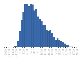
[ What is Monte Carlo Simulation? ]

Preface

There are many things that faster computers have made possible in recent years. For scientists, engineers, statisticians, managers, investors, and others, computers have made it possible to create models that simulate reality and aid in making predictions. One of the methods for simulating real systems is the ability to take into account randomness by investigating hundreds of thousands of different scenarios. The results are then compiled and used to make decisions. This is what Monte Carlo simulation is about.

Monte Carlo simulation is often used in business for risk and decision analysis, to help make decisions given uncertainties in market trends, fluctuations, and other uncertain factors. In the science and engineering communities, MC simulation is often used for uncertainty analysis, optimization, and reliability-based design. In manufacturing, MC methods are used to help allocate tolerances in order to reduce cost. There are certainly other fields that employ MC methods, and there are also times when MC is not practical (for extremely large problems, computer speed is still an issue). However, MC continues to gain popularity, and is often used as a benchmark for evaluating other statistical methods.

This article will guide you through the process of performing a Monte Carlo simulation using Microsoft Excel. Although Excel will not always be the best place to run a scientific simulation, the basics are easily explained with just a few simple examples. If you frequently use Excel for modeling, whether for engineering design or financial analysis, I highly suggest one of the Excel add-ins listed below.

MC Simulation Software

The popularity of Monte Carlo methods have led to a number of superb commercial tools. The programs listed below work directly with Excel as add-ins. Crystal Ball and @Risk are the two most popular and are very high quality (which you would expect from the price). Risk Solver is an amazing new add-in created by the makers of the famous Excel Solver add-in. Risk Solver runs at lightning speed and certainly rivals Crystal Ball and @Risk.

Excel Add-Ins
@Risk	$1,195
Crystal Ball	$995
Risk Solver	$995
DFSS Master	$399
RiskAMP Add-In for Excel	$129.95
Risk Analyzer	$49.95
Actual prices may vary from those listed.

[ What is Monte Carlo Simulation? ]

Books featuring Crystal Ball

Business Modeling

> Essentials of Business Statistics, 1/e, by: James R. Evans

> Quantitative Business Modeling, 1/e, by: Jack R. Meredith, Scott M. Shafer, Efraim Turban

> Quantitative Methods for Business, 8/e, by: David R. Anderson, Dennis J. Sweeney, Thomas A. Williams

> The Art of Modeling with Spreadsheets: Management Science, Spreadsheet Engineering, and Modeling Craft, by: Stephen G. Powell, Dartmouth College, and Kenneth R. Baker, Dartmouth College

Decision Analysis

> Statistics, Data Analysis, and Decision Modeling, 2/e, by: James R. Evans and David L. Olson

> Spreadsheet Modeling and Decision Analysis, 4/e, by: Cliff Ragsdale, Georgia Southern University

Risk Analysis

> Applied Risk Analysis: Moving Beyond Uncertainty, by: Johnathan Mun, Decisioneering

> Introduction to Simulation and Risk Analysis, 2/e, by: James R. Evans, University of Cincinnati, and David L. Olson, Texas A&M University

Management Science

> Management Science and Decision Technology, by: Jeff Camm and James Evans

> Managerial Decision Modeling with Spreadsheets, by: Barry Render, Ralph M. Stair Jr., and Nagraj Balakrishnan

> Management Decision Making: Spreadsheet Modeling, Analysis, and Applications, by: George E. Monahan

> An Introduction to Management Science: Quantitative Approaches to Decision Making, 10/e, by: David Ray Anderson, Dennis J. Sweeney, Thomas Arthur Williams

> Introduction to Management Science, 7/e, by: Bernard W. Taylor, III, Virginia Polytechnic Institute & State University

> Data Models and Decisions: The Fundamentals of Management Science, by: Dimitris Bertsimas, MIT Sloan School of Management, and Robert Freund, MIT Sloan School of Management

Project Management

> Project Management: A Managerial Approach, 5/e, by: Jack R. Meredith and Samuel J. Mantel

> Project Management in Practice, by: Samuel J. Mantel (Editor), Jack R. Meredith, Scott M. Shafer, Sutton, Margaret Sutton, Jr., Samuel J. Mantel

Real Options Analysis

> Real Options Analysis: Tools and Techniques for Valuing Strategic Investments & Decisions, by: Dr. Johnathan Mun

> Real Options Analysis Course: Business Cases and Software Applications, by: Dr. Johnathan Mun

Источник

Need more help?

Need more help?

Key Takeaways

Monte Carlo Simulation

When to Use the Monte Carlo Simulation

Game of Dice

Step 1: Dice Rolling Events

Step 2: Range of Outcomes

Step 3: Conclusions

Step 4: Number of Dice Rolls

Step 5: Simulation

Step 6: Probability

What is Monte Carlo Simulation?

Describe Monte Carlo

The Monte Carlo Simulation Formula

Distribution Curves

Uniform Distribution

Normal (Gaussian) Distribution

Lognormal Distribution

Poisson Distribution

Building The Model

Input Variables

First Simulation

1,000 Simulations

Summary Statistics

Get the Download

Now What?

Chandoo

INTRODUCTION

DATA TABLE BASICS

Where is the Data Table Function

Blue Sky Mine Co

1 WAY DATA TABLES

What if my Data is in Rows?

What if I want to vary the inputs by a certain Percentage ?

2 WAY DATA TABLES

What about varying by Percentages?

MONITORING MULTIPLE VARIABLES

MULTIWAY DATA TABLES

MONTE CARLO SIMULATIONS IN EXCEL

First some statistics.

Monte Carlo simulations

Advanced Monte Carlo Simulations

ITERATED FUNCTIONS INCLUDING FRACTALS

Excel Mandelbrot

DOWNLOAD EXAMPLE WORKBOOKS

FINAL THOUGHTS

Speed

VBA

Cell Contents

Further Reading & References

Added by Chandoo

Get FREE Excel + Power BI Tips

Welcome to Chandoo.org

Related Tips

205 Responses to “Data Tables & Monte Carlo Simulations in Excel – A Comprehensive Guide”

Leave a Reply

MC Simulation Software

Excel Add-Ins

Books featuring Crystal Ball