
«Algorithms» redirects here. For the subfield of computer science, see Analysis of algorithms.

Flow-chart of an algorithm (Euclides algorithm’s) for calculating the greatest common divisor (g.c.d.) of two numbers a and b in locations named A and B. The algorithm proceeds by successive subtractions in two loops: IF the test B ≥ A yields «yes» or «true» (more accurately, the number b in location B is greater than or equal to the number a in location A) THEN, the algorithm specifies B ← B − A (meaning the number b − a replaces the old b). Similarly, IF A > B, THEN A ← A − B. The process terminates when (the contents of) B is 0, yielding the g.c.d. in A. (Algorithm derived from Scott 2009:13; symbols and drawing style from Tausworthe 1977).

Ada Lovelace’s diagram from «note G», the first published computer algorithm
In mathematics and computer science, an algorithm () is a finite sequence of rigorous instructions, typically used to solve a class of specific problems or to perform a computation.[1] Algorithms are used as specifications for performing calculations and data processing. More advanced algorithms can use conditionals to divert the code execution through various routes (referred to as automated decision-making) and deduce valid inferences (referred to as automated reasoning), achieving automation eventually. Using human characteristics as descriptors of machines in metaphorical ways was already practiced by Alan Turing with terms such as «memory», «search» and «stimulus».[2]
In contrast, a heuristic is an approach to problem solving that may not be fully specified or may not guarantee correct or optimal results, especially in problem domains where there is no well-defined correct or optimal result.[3]
As an effective method, an algorithm can be expressed within a finite amount of space and time,[4] and in a well-defined formal language[5] for calculating a function.[6] Starting from an initial state and initial input (perhaps empty),[7] the instructions describe a computation that, when executed, proceeds through a finite[8] number of well-defined successive states, eventually producing «output»[9] and terminating at a final ending state. The transition from one state to the next is not necessarily deterministic; some algorithms, known as randomized algorithms, incorporate random input.[10]
History[edit]
Ancient algorithms[edit]
Since antiquity, step-by-step procedures for solving mathematical problems have been attested. This includes Babylonian mathematics (around 2500 BC),[11] Egyptian mathematics (around 1550 BC),[11] Indian mathematics (around 800 BC and later; e.g. Shulba Sutras, Kerala School, and Brāhmasphuṭasiddhānta),[12][13] Greek mathematics (around 240 BC, e.g. sieve of Eratosthenes and Euclidean algorithm),[14] and Arabic mathematics (9th century, e.g. cryptographic algorithms for code-breaking based on frequency analysis).[15]
Al-Khwarizmi and the term algorithm[edit]
Around 825, Muhammad ibn Musa al-Khwarizmi wrote kitāb al-ḥisāb al-hindī («Book of Indian computation») and kitab al-jam’ wa’l-tafriq al-ḥisāb al-hindī («Addition and subtraction in Indian arithmetic»). Both of these texts are lost in the original Arabic at this time. (However, his other book on algebra remains.)[16]
In the early 12th century, Latin translations of said al-Khwarizmi texts involving the Hindu–Arabic numeral system and arithmetic appeared: Liber Alghoarismi de practica arismetrice (attributed to John of Seville) and Liber Algorismi de numero Indorum (attributed to Adelard of Bath).[17] Hereby, alghoarismi or algorismi is the Latinization of Al-Khwarizmi’s name; the text starts with the phrase Dixit Algorismi («Thus spoke Al-Khwarizmi»).[18]
In 1240, Alexander of Villedieu writes a Latin text titled Carmen de Algorismo. It begins with:
Haec algorismus ars praesens dicitur, in qua / Talibus Indorum fruimur bis quinque figuris.
which translates to:
Algorism is the art by which at present we use those Indian figures, which number two times five.
The poem is a few hundred lines long and summarizes the art of calculating with the new styled Indian dice (Tali Indorum), or Hindu numerals.[19]
English evolution of the word[edit]
Around 1230, the English word algorism is attested and then by Chaucer in 1391. English adopted the French term.[20][21]
In the 15th century, under the influence of the Greek word ἀριθμός (arithmos, «number»; cf. «arithmetic»), the Latin word was altered to algorithmus.
In 1656, in the English dictionary Glossographia, it says:[22]
Algorism ([Latin] algorismus) the Art or use of Cyphers, or of numbering by Cyphers; skill in accounting.
Augrime ([Latin] algorithmus) skil in accounting or numbring.
In 1658, in the first edition of The New World of English Words, it says:[23]
Algorithme, (a word compounded of Arabick and Spanish,) the art of reckoning by Cyphers.
In 1706, in the sixth edition of The New World of English Words, it says:[24]
Algorithm, the Art of computing or reckoning by numbers, which contains the five principle Rules of Arithmetick, viz. Numeration, Addition, Subtraction, Multiplication and Division; to which may be added Extraction of Roots: It is also call’d Logistica Numeralis.
Algorism, the practical Operation in the several Parts of Specious Arithmetick or Algebra; sometimes it is taken for the Practice of Common Arithmetick by the ten Numeral Figures.
In 1751, in the Young Algebraist’s Companion, Daniel Fenning contrasts the terms algorism and algorithm as follows:[25]
Algorithm signifies the first Principles, and Algorism the practical Part, or knowing how to put the Algorithm in Practice.
Since at least 1811, the term algorithm is attested to mean a «step-by-step procedure» in English.[26][27]
In 1842, in the Dictionary of Science, Literature and Art, it says:
ALGORITHM, signifies the art of computing in reference to some particular subject, or in some particular way; as the algorithm of numbers; the algorithm of the differential calculus.[28]
Machine usage[edit]
In 1928, a partial formalization of the modern concept of algorithm began with attempts to solve the Entscheidungsproblem (decision problem) posed by David Hilbert. Later formalizations were framed as attempts to define «effective calculability»[29] or «effective method».[30] Those formalizations included the Gödel–Herbrand–Kleene recursive functions of 1930, 1934 and 1935, Alonzo Church’s lambda calculus of 1936, Emil Post’s Formulation 1 of 1936, and Alan Turing’s Turing machines of 1936–37 and 1939.
Informal definition[edit]
For a detailed presentation of the various points of view on the definition of «algorithm», see Algorithm characterizations.
An informal definition could be «a set of rules that precisely defines a sequence of operations»,[31][need quotation to verify] which would include all computer programs (including programs that do not perform numeric calculations), and (for example) any prescribed bureaucratic procedure[32]
or cook-book recipe.[33]
In general, a program is only an algorithm if it stops eventually[34]—even though infinite loops may sometimes prove desirable.
A prototypical example of an algorithm is the Euclidean algorithm, which is used to determine the maximum common divisor of two integers; an example (there are others) is described by the flowchart above and as an example in a later section.
Boolos, Jeffrey & 1974, 1999 offer an informal meaning of the word «algorithm» in the following quotation:
No human being can write fast enough, or long enough, or small enough† ( †»smaller and smaller without limit … you’d be trying to write on molecules, on atoms, on electrons») to list all members of an enumerably infinite set by writing out their names, one after another, in some notation. But humans can do something equally useful, in the case of certain enumerably infinite sets: They can give explicit instructions for determining the nth member of the set, for arbitrary finite n. Such instructions are to be given quite explicitly, in a form in which they could be followed by a computing machine, or by a human who is capable of carrying out only very elementary operations on symbols.[35]
An «enumerably infinite set» is one whose elements can be put into one-to-one correspondence with the integers. Thus Boolos and Jeffrey are saying that an algorithm implies instructions for a process that «creates» output integers from an arbitrary «input» integer or integers that, in theory, can be arbitrarily large. For example, an algorithm can be an algebraic equation such as y = m + n (i.e., two arbitrary «input variables» m and n that produce an output y), but various authors’ attempts to define the notion indicate that the word implies much more than this, something on the order of (for the addition example):
- Precise instructions (in a language understood by «the computer»)[36] for a fast, efficient, «good»[37] process that specifies the «moves» of «the computer» (machine or human, equipped with the necessary internally contained information and capabilities)[38] to find, decode, and then process arbitrary input integers/symbols m and n, symbols + and = … and «effectively»[39] produce, in a «reasonable» time,[40] output-integer y at a specified place and in a specified format.
The concept of algorithm is also used to define the notion of decidability—a notion that is central for explaining how formal systems come into being starting from a small set of axioms and rules. In logic, the time that an algorithm requires to complete cannot be measured, as it is not apparently related to the customary physical dimension. From such uncertainties, that characterize ongoing work, stems the unavailability of a definition of algorithm that suits both concrete (in some sense) and abstract usage of the term.
Most algorithms are intended to be implemented as computer programs. However, algorithms are also implemented by other means, such as in a biological neural network (for example, the human brain implementing arithmetic or an insect looking for food), in an electrical circuit, or in a mechanical device.
Formalization[edit]
Algorithms are essential to the way computers process data. Many computer programs contain algorithms that detail the specific instructions a computer should perform—in a specific order—to carry out a specified task, such as calculating employees’ paychecks or printing students’ report cards. Thus, an algorithm can be considered to be any sequence of operations that can be simulated by a Turing-complete system. Authors who assert this thesis include Minsky (1967), Savage (1987), and Gurevich (2000):
Minsky: «But we will also maintain, with Turing … that any procedure which could «naturally» be called effective, can, in fact, be realized by a (simple) machine. Although this may seem extreme, the arguments … in its favor are hard to refute».[41]
Gurevich: «… Turing’s informal argument in favor of his thesis justifies a stronger thesis: every algorithm can be simulated by a Turing machine … according to Savage [1987], an algorithm is a computational process defined by a Turing machine».[42]
Turing machines can define computational processes that do not terminate. The informal definitions of algorithms generally require that the algorithm always terminates. This requirement renders the task of deciding whether a formal procedure is an algorithm impossible in the general case—due to a major theorem of computability theory known as the halting problem.
Typically, when an algorithm is associated with processing information, data can be read from an input source, written to an output device and stored for further processing. Stored data are regarded as part of the internal state of the entity performing the algorithm. In practice, the state is stored in one or more data structures.
For some of these computational processes, the algorithm must be rigorously defined: and specified in the way it applies in all possible circumstances that could arise. This means that any conditional steps must be systematically dealt with, case by case; the criteria for each case must be clear (and computable).
Because an algorithm is a precise list of precise steps, the order of computation is always crucial to the functioning of the algorithm. Instructions are usually assumed to be listed explicitly, and are described as starting «from the top» and going «down to the bottom»—an idea that is described more formally by flow of control.
So far, the discussion on the formalization of an algorithm has assumed the premises of imperative programming. This is the most common conception—one which attempts to describe a task in discrete, «mechanical» means. Unique to this conception of formalized algorithms is the assignment operation, which sets the value of a variable. It derives from the intuition of «memory» as a scratchpad. An example of such an assignment can be found below.
For some alternate conceptions of what constitutes an algorithm, see functional programming and logic programming.
Expressing algorithms[edit]
Algorithms can be expressed in many kinds of notation, including natural languages, pseudocode, flowcharts, drakon-charts, programming languages or control tables (processed by interpreters). Natural language expressions of algorithms tend to be verbose and ambiguous, and are rarely used for complex or technical algorithms. Pseudocode, flowcharts, drakon-charts and control tables are structured ways to express algorithms that avoid many of the ambiguities common in the statements based on natural language. Programming languages are primarily intended for expressing algorithms in a form that can be executed by a computer, but are also often used as a way to define or document algorithms.
There is a wide variety of representations possible and one can express a given Turing machine program as a sequence of machine tables (see finite-state machine, state transition table and control table for more), as flowcharts and drakon-charts (see state diagram for more), or as a form of rudimentary machine code or assembly code called «sets of quadruples» (see Turing machine for more).
Representations of algorithms can be classed into three accepted levels of Turing machine description, as follows:[43]
- 1 High-level description
- «…prose to describe an algorithm, ignoring the implementation details. At this level, we do not need to mention how the machine manages its tape or head.»
- 2 Implementation description
- «…prose used to define the way the Turing machine uses its head and the way that it stores data on its tape. At this level, we do not give details of states or transition function.»
- 3 Formal description
- Most detailed, «lowest level», gives the Turing machine’s «state table».
For an example of the simple algorithm «Add m+n» described in all three levels, see Examples.
Design[edit]
See also: Algorithm § By design paradigm
Algorithm design refers to a method or a mathematical process for problem-solving and engineering algorithms. The design of algorithms is part of many solution theories, such as divide-and-conquer or dynamic programming within operation research. Techniques for designing and implementing algorithm designs are also called algorithm design patterns,[44] with examples including the template method pattern and the decorator pattern.
One of the most important aspects of algorithm design is resource (run-time, memory usage) efficiency; the big O notation is used to describe e.g. an algorithm’s run-time growth as the size of its input increases.
Typical steps in the development of algorithms:
- Problem definition
- Development of a model
- Specification of the algorithm
- Designing an algorithm
- Checking the correctness of the algorithm
- Analysis of algorithm
- Implementation of algorithm
- Program testing
- Documentation preparation[clarification needed]
Computer algorithms[edit]


Flowchart examples of the canonical Böhm-Jacopini structures: the SEQUENCE (rectangles descending the page), the WHILE-DO and the IF-THEN-ELSE. The three structures are made of the primitive conditional GOTO (IF test THEN GOTO step xxx, shown as diamond), the unconditional GOTO (rectangle), various assignment operators (rectangle), and HALT (rectangle). Nesting of these structures inside assignment-blocks results in complex diagrams (cf. Tausworthe 1977:100, 114).
«Elegant» (compact) programs, «good» (fast) programs : The notion of «simplicity and elegance» appears informally in Knuth and precisely in Chaitin:
- Knuth: » … we want good algorithms in some loosely defined aesthetic sense. One criterion … is the length of time taken to perform the algorithm …. Other criteria are adaptability of the algorithm to computers, its simplicity, and elegance, etc.»[45]
- Chaitin: » … a program is ‘elegant,’ by which I mean that it’s the smallest possible program for producing the output that it does»[46]
Chaitin prefaces his definition with: «I’ll show you can’t prove that a program is ‘elegant‘«—such a proof would solve the Halting problem (ibid).
Algorithm versus function computable by an algorithm: For a given function multiple algorithms may exist. This is true, even without expanding the available instruction set available to the programmer. Rogers observes that «It is … important to distinguish between the notion of algorithm, i.e. procedure and the notion of function computable by algorithm, i.e. mapping yielded by procedure. The same function may have several different algorithms».[47]
Unfortunately, there may be a tradeoff between goodness (speed) and elegance (compactness)—an elegant program may take more steps to complete a computation than one less elegant. An example that uses Euclid’s algorithm appears below.
Computers (and computors), models of computation: A computer (or human «computer»[48]) is a restricted type of machine, a «discrete deterministic mechanical device»[49] that blindly follows its instructions.[50] Melzak’s and Lambek’s primitive models[51] reduced this notion to four elements: (i) discrete, distinguishable locations, (ii) discrete, indistinguishable counters[52] (iii) an agent, and (iv) a list of instructions that are effective relative to the capability of the agent.[53]
Minsky describes a more congenial variation of Lambek’s «abacus» model in his «Very Simple Bases for Computability».[54] Minsky’s machine proceeds sequentially through its five (or six, depending on how one counts) instructions unless either a conditional IF-THEN GOTO or an unconditional GOTO changes program flow out of sequence. Besides HALT, Minsky’s machine includes three assignment (replacement, substitution)[55] operations: ZERO (e.g. the contents of location replaced by 0: L ← 0), SUCCESSOR (e.g. L ← L+1), and DECREMENT (e.g. L ← L − 1).[56] Rarely must a programmer write «code» with such a limited instruction set. But Minsky shows (as do Melzak and Lambek) that his machine is Turing complete with only four general types of instructions: conditional GOTO, unconditional GOTO, assignment/replacement/substitution, and HALT. However, a few different assignment instructions (e.g. DECREMENT, INCREMENT, and ZERO/CLEAR/EMPTY for a Minsky machine) are also required for Turing-completeness; their exact specification is somewhat up to the designer. The unconditional GOTO is convenient; it can be constructed by initializing a dedicated location to zero e.g. the instruction » Z ← 0 «; thereafter the instruction IF Z=0 THEN GOTO xxx is unconditional.
Simulation of an algorithm: computer (computor) language: Knuth advises the reader that «the best way to learn an algorithm is to try it . . . immediately take pen and paper and work through an example».[57] But what about a simulation or execution of the real thing? The programmer must translate the algorithm into a language that the simulator/computer/computor can effectively execute. Stone gives an example of this: when computing the roots of a quadratic equation the computer must know how to take a square root. If they don’t, then the algorithm, to be effective, must provide a set of rules for extracting a square root.[58]
This means that the programmer must know a «language» that is effective relative to the target computing agent (computer/computor).
But what model should be used for the simulation? Van Emde Boas observes «even if we base complexity theory on abstract instead of concrete machines, the arbitrariness of the choice of a model remains. It is at this point that the notion of simulation enters».[59] When speed is being measured, the instruction set matters. For example, the subprogram in Euclid’s algorithm to compute the remainder would execute much faster if the programmer had a «modulus» instruction available rather than just subtraction (or worse: just Minsky’s «decrement»).
Structured programming, canonical structures: Per the Church–Turing thesis, any algorithm can be computed by a model known to be Turing complete, and per Minsky’s demonstrations, Turing completeness requires only four instruction types—conditional GOTO, unconditional GOTO, assignment, HALT. Kemeny and Kurtz observe that, while «undisciplined» use of unconditional GOTOs and conditional IF-THEN GOTOs can result in «spaghetti code», a programmer can write structured programs using only these instructions; on the other hand «it is also possible, and not too hard, to write badly structured programs in a structured language».[60] Tausworthe augments the three Böhm-Jacopini canonical structures:[61] SEQUENCE, IF-THEN-ELSE, and WHILE-DO, with two more: DO-WHILE and CASE.[62] An additional benefit of a structured program is that it lends itself to proofs of correctness using mathematical induction.[63]
Canonical flowchart symbols[64]: The graphical aide called a flowchart offers a way to describe and document an algorithm (and a computer program corresponding to it). Like the program flow of a Minsky machine, a flowchart always starts at the top of a page and proceeds down. Its primary symbols are only four: the directed arrow showing program flow, the rectangle (SEQUENCE, GOTO), the diamond (IF-THEN-ELSE), and the dot (OR-tie). The Böhm–Jacopini canonical structures are made of these primitive shapes. Sub-structures can «nest» in rectangles, but only if a single exit occurs from the superstructure. The symbols and their use to build the canonical structures are shown in the diagram.
Examples[edit]
Algorithm example[edit]
One of the simplest algorithms is to find the largest number in a list of numbers of random order. Finding the solution requires looking at every number in the list. From this follows a simple algorithm, which can be stated in a high-level description in English prose, as:
High-level description:
- If there are no numbers in the set, then there is no highest number.
- Assume the first number in the set is the largest number in the set.
- For each remaining number in the set: if this number is larger than the current largest number, consider this number to be the largest number in the set.
- When there are no numbers left in the set to iterate over, consider the current largest number to be the largest number of the set.
(Quasi-)formal description:
Written in prose but much closer to the high-level language of a computer program, the following is the more formal coding of the algorithm in pseudocode or pidgin code:
Algorithm LargestNumber
Input: A list of numbers L.
Output: The largest number in the list L.
if L.size = 0 return null
largest ← L[0]
for each item in L, do
    if item > largest, then
        largest ← item
return largest
- «←» denotes assignment. For instance, «largest ← item» means that the value of largest changes to the value of item.
- «return» terminates the algorithm and outputs the following value.
Euclid’s algorithm[edit]
In mathematics, the Euclidean algorithm or Euclid’s algorithm, is an efficient method for computing the greatest common divisor (GCD) of two integers (numbers), the largest number that divides them both without a remainder. It is named after the ancient Greek mathematician Euclid, who first described it in his Elements (c. 300 BC).[65] It is one of the oldest algorithms in common use. It can be used to reduce fractions to their simplest form, and is a part of many other number-theoretic and cryptographic calculations.
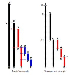
The example-diagram of Euclid’s algorithm from T.L. Heath (1908), with more detail added. Euclid does not go beyond a third measuring and gives no numerical examples. Nicomachus gives the example of 49 and 21: «I subtract the less from the greater; 28 is left; then again I subtract from this the same 21 (for this is possible); 7 is left; I subtract this from 21, 14 is left; from which I again subtract 7 (for this is possible); 7 is left, but 7 cannot be subtracted from 7.» Heath comments that «The last phrase is curious, but the meaning of it is obvious enough, as also the meaning of the phrase about ending ‘at one and the same number’.»(Heath 1908:300).
Euclid poses the problem thus: «Given two numbers not prime to one another, to find their greatest common measure». He defines «A number [to be] a multitude composed of units»: a counting number, a positive integer not including zero. To «measure» is to place a shorter measuring length s successively (q times) along longer length l until the remaining portion r is less than the shorter length s.[66] In modern words, remainder r = l − q×s, q being the quotient, or remainder r is the «modulus», the integer-fractional part left over after the division.[67]
For Euclid’s method to succeed, the starting lengths must satisfy two requirements: (i) the lengths must not be zero, AND (ii) the subtraction must be «proper»; i.e., a test must guarantee that the smaller of the two numbers is subtracted from the larger (or the two can be equal so their subtraction yields zero).
Euclid’s original proof adds a third requirement: the two lengths must not be prime to one another. Euclid stipulated this so that he could construct a reductio ad absurdum proof that the two numbers’ common measure is in fact the greatest.[68] While Nicomachus’ algorithm is the same as Euclid’s, when the numbers are prime to one another, it yields the number «1» for their common measure. So, to be precise, the following is really Nicomachus’ algorithm.
A graphical expression of Euclid’s algorithm to find the greatest common divisor for 1599 and 650
 1599 = 650×2 + 299
 650 = 299×2 + 52
 299 = 52×5 + 39
 52 = 39×1 + 13
 39 = 13×3 + 0
Computer language for Euclid’s algorithm[edit]
Only a few instruction types are required to execute Euclid’s algorithm—some logical tests (conditional GOTO), unconditional GOTO, assignment (replacement), and subtraction.
- A location is symbolized by upper case letter(s), e.g. S, A, etc.
- The varying quantity (number) in a location is written in lower case letter(s) and (usually) associated with the location’s name. For example, location L at the start might contain the number l = 3009.
An inelegant program for Euclid’s algorithm[edit]

«Inelegant» is a translation of Knuth’s version of the algorithm with a subtraction-based remainder-loop replacing his use of division (or a «modulus» instruction). Derived from Knuth 1973:2–4. Depending on the two numbers «Inelegant» may compute the g.c.d. in fewer steps than «Elegant».
The following algorithm is framed as Knuth’s four-step version of Euclid’s and Nicomachus’, but, rather than using division to find the remainder, it uses successive subtractions of the shorter length s from the remaining length r until r is less than s. The high-level description, shown in boldface, is adapted from Knuth 1973:2–4:
INPUT:
1 [Into two locations L and S put the numbers l and s that represent the two lengths]:
INPUT L, S
2 [Initialize R: make the remaining length r equal to the starting/initial/input length l]:
R ← L
E0: [Ensure r ≥ s.]
3 [Ensure the smaller of the two numbers is in S and the larger in R]:
IF R > S THEN
the contents of L is the larger number so skip over the exchange-steps 4, 5 and 6:
GOTO step 7
ELSE
swap the contents of R and S.
4 L ← R (this first step is redundant, but is useful for later discussion).
5 R ← S
6 S ← L
E1: [Find remainder]: Until the remaining length r in R is less than the shorter length s in S, repeatedly subtract the measuring number s in S from the remaining length r in R.
7 IF S > R THEN
done measuring so
GOTO 10
ELSE
measure again,
8 R ← R − S
9 [Remainder-loop]:
GOTO 7.
E2: [Is the remainder zero?]: EITHER (i) the last measure was exact, the remainder in R is zero, and the program can halt, OR (ii) the algorithm must continue: the last measure left a remainder in R less than measuring number in S.
10 IF R = 0 THEN
done so
GOTO step 15
ELSE
CONTINUE TO step 11,
E3: [Interchange s and r]: The nut of Euclid’s algorithm. Use remainder r to measure what was previously smaller number s; L serves as a temporary location.
11 L ← R
12 R ← S
13 S ← L
14 [Repeat the measuring process]:
GOTO 7
OUTPUT:
15 [Done. S contains the greatest common divisor]:
PRINT S
DONE:
16 HALT, END, STOP.
An elegant program for Euclid’s algorithm[edit]
The following version of Euclid’s algorithm requires only six core instructions to do what thirteen are required to do by «Inelegant»; worse, «Inelegant» requires more types of instructions.[clarify] The flowchart of «Elegant» can be found at the top of this article. In the (unstructured) Basic language, the steps are numbered, and the instruction LET [] = [] is the assignment instruction symbolized by ←.
  5 REM Euclid's algorithm for greatest common divisor
  6 PRINT "Type two integers greater than 0"
  10 INPUT A,B
  20 IF B=0 THEN GOTO 80
  30 IF A > B THEN GOTO 60
  40 LET B=B-A
  50 GOTO 20
  60 LET A=A-B
  70 GOTO 20
  80 PRINT A
  90 END
How «Elegant» works: In place of an outer «Euclid loop», «Elegant» shifts back and forth between two «co-loops», an A > B loop that computes A ← A − B, and a B ≤ A loop that computes B ← B − A. This works because, when at last the minuend M is less than or equal to the subtrahend S (Difference = Minuend − Subtrahend), the minuend can become s (the new measuring length) and the subtrahend can become the new r (the length to be measured); in other words the «sense» of the subtraction reverses.
The following version can be used with programming languages from the C-family:
// Euclid's algorithm for greatest common divisor
int euclidAlgorithm (int A, int B) {
     A = abs(A);
     B = abs(B);
     while (B != 0) {
          while (A > B) {
               A = A-B;
          }
          B = B-A;
     }
     return A;
}
Testing the Euclid algorithms[edit]
Does an algorithm do what its author wants it to do? A few test cases usually give some confidence in the core functionality. But tests are not enough. For test cases, one source[69] uses 3009 and 884. Knuth suggested 40902, 24140. Another interesting case is the two relatively prime numbers 14157 and 5950.
But «exceptional cases»[70] must be identified and tested. Will «Inelegant» perform properly when R > S, S > R, R = S? Ditto for «Elegant»: B > A, A > B, A = B? (Yes to all). What happens when one number is zero, both numbers are zero? («Inelegant» computes forever in all cases; «Elegant» computes forever when A = 0.) What happens if negative numbers are entered? Fractional numbers? If the input numbers, i.e. the domain of the function computed by the algorithm/program, is to include only positive integers including zero, then the failures at zero indicate that the algorithm (and the program that instantiates it) is a partial function rather than a total function. A notable failure due to exceptions is the Ariane 5 Flight 501 rocket failure (June 4, 1996).
Proof of program correctness by use of mathematical induction: Knuth demonstrates the application of mathematical induction to an «extended» version of Euclid’s algorithm, and he proposes «a general method applicable to proving the validity of any algorithm».[71] Tausworthe proposes that a measure of the complexity of a program be the length of its correctness proof.[72]
Measuring and improving the Euclid algorithms[edit]
Elegance (compactness) versus goodness (speed): With only six core instructions, «Elegant» is the clear winner, compared to «Inelegant» at thirteen instructions. However, «Inelegant» is faster (it arrives at HALT in fewer steps). Algorithm analysis[73] indicates why this is the case: «Elegant» does two conditional tests in every subtraction loop, whereas «Inelegant» only does one. As the algorithm (usually) requires many loop-throughs, on average much time is wasted doing a «B = 0?» test that is needed only after the remainder is computed.
Can the algorithms be improved?: Once the programmer judges a program «fit» and «effective»—that is, it computes the function intended by its author—then the question becomes, can it be improved?
The compactness of «Inelegant» can be improved by the elimination of five steps. But Chaitin proved that compacting an algorithm cannot be automated by a generalized algorithm;[74] rather, it can only be done heuristically; i.e., by exhaustive search (examples to be found at Busy beaver), trial and error, cleverness, insight, application of inductive reasoning, etc. Observe that steps 4, 5 and 6 are repeated in steps 11, 12 and 13. Comparison with «Elegant» provides a hint that these steps, together with steps 2 and 3, can be eliminated. This reduces the number of core instructions from thirteen to eight, which makes it «more elegant» than «Elegant», at nine steps.
The speed of «Elegant» can be improved by moving the «B=0?» test outside of the two subtraction loops. This change calls for the addition of three instructions (B = 0?, A = 0?, GOTO). Now «Elegant» computes the example-numbers faster; whether this is always the case for any given A, B, and R, S would require a detailed analysis.
Algorithmic analysis[edit]
It is frequently important to know how much of a particular resource (such as time or storage) is theoretically required for a given algorithm. Methods have been developed for the analysis of algorithms to obtain such quantitative answers (estimates); for example, an algorithm which adds up the elements of a list of n numbers would have a time requirement of O(n), using big O notation. At all times the algorithm only needs to remember two values: the sum of all the elements so far, and its current position in the input list. Therefore, it is said to have a space requirement of O(1), if the space required to store the input numbers is not counted, or O(n) if it is counted.
Different algorithms may complete the same task with a different set of instructions in less or more time, space, or ‘effort’ than others. For example, a binary search algorithm (with cost O(log n)) outperforms a sequential search (cost O(n) ) when used for table lookups on sorted lists or arrays.
Formal versus empirical[edit]
The analysis, and study of algorithms is a discipline of computer science, and is often practiced abstractly without the use of a specific programming language or implementation. In this sense, algorithm analysis resembles other mathematical disciplines in that it focuses on the underlying properties of the algorithm and not on the specifics of any particular implementation. Usually pseudocode is used for analysis as it is the simplest and most general representation. However, ultimately, most algorithms are usually implemented on particular hardware/software platforms and their algorithmic efficiency is eventually put to the test using real code. For the solution of a «one off» problem, the efficiency of a particular algorithm may not have significant consequences (unless n is extremely large) but for algorithms designed for fast interactive, commercial or long life scientific usage it may be critical. Scaling from small n to large n frequently exposes inefficient algorithms that are otherwise benign.
Empirical testing is useful because it may uncover unexpected interactions that affect performance. Benchmarks may be used to compare before/after potential improvements to an algorithm after program optimization.
Empirical tests cannot replace formal analysis, though, and are not trivial to perform in a fair manner.[75]
Execution efficiency[edit]
To illustrate the potential improvements possible even in well-established algorithms, a recent significant innovation, relating to FFT algorithms (used heavily in the field of image processing), can decrease processing time up to 1,000 times for applications like medical imaging.[76] In general, speed improvements depend on special properties of the problem, which are very common in practical applications.[77] Speedups of this magnitude enable computing devices that make extensive use of image processing (like digital cameras and medical equipment) to consume less power.
Classification[edit]
There are various ways to classify algorithms, each with its own merits.
By implementation[edit]
One way to classify algorithms is by implementation means.
int gcd(int A, int B) { if (B == 0) return A; else if (A > B) return gcd(A-B,B); else return gcd(A,B-A); } |
| Recursive C implementation of Euclid’s algorithm from the above flowchart |
- Recursion
- A recursive algorithm is one that invokes (makes reference to) itself repeatedly until a certain condition (also known as termination condition) matches, which is a method common to functional programming. Iterative algorithms use repetitive constructs like loops and sometimes additional data structures like stacks to solve the given problems. Some problems are naturally suited for one implementation or the other. For example, towers of Hanoi is well understood using recursive implementation. Every recursive version has an equivalent (but possibly more or less complex) iterative version, and vice versa.
- Logical
- An algorithm may be viewed as controlled logical deduction. This notion may be expressed as: Algorithm = logic + control.[78] The logic component expresses the axioms that may be used in the computation and the control component determines the way in which deduction is applied to the axioms. This is the basis for the logic programming paradigm. In pure logic programming languages, the control component is fixed and algorithms are specified by supplying only the logic component. The appeal of this approach is the elegant semantics: a change in the axioms produces a well-defined change in the algorithm.
- Serial, parallel or distributed
- Algorithms are usually discussed with the assumption that computers execute one instruction of an algorithm at a time. Those computers are sometimes called serial computers. An algorithm designed for such an environment is called a serial algorithm, as opposed to parallel algorithms or distributed algorithms. Parallel algorithms are algorithms that take advantage of computer architectures where multiple processors can work on a problem at the same time. Distributed algorithms are algorithms that use multiple machines connected with a computer network. Parallel and distributed algorithms divide the problem into more symmetrical or asymmetrical subproblems and collect the results back together. For example, a CPU would be an example of a parallel algorithm. The resource consumption in such algorithms is not only processor cycles on each processor but also the communication overhead between the processors. Some sorting algorithms can be parallelized efficiently, but their communication overhead is expensive. Iterative algorithms are generally parallelizable, but some problems have no parallel algorithms and are called inherently serial problems.
- Deterministic or non-deterministic
- Deterministic algorithms solve the problem with exact decision at every step of the algorithm whereas non-deterministic algorithms solve problems via guessing although typical guesses are made more accurate through the use of heuristics.
- Exact or approximate
- While many algorithms reach an exact solution, approximation algorithms seek an approximation that is closer to the true solution. The approximation can be reached by either using a deterministic or a random strategy. Such algorithms have practical value for many hard problems. One of the examples of an approximate algorithm is the Knapsack problem, where there is a set of given items. Its goal is to pack the knapsack to get the maximum total value. Each item has some weight and some value. Total weight that can be carried is no more than some fixed number X. So, the solution must consider weights of items as well as their value.[79]
- Quantum algorithm
- They run on a realistic model of quantum computation. The term is usually used for those algorithms which seem inherently quantum, or use some essential feature of Quantum computing such as quantum superposition or quantum entanglement.
By design paradigm[edit]
Another way of classifying algorithms is by their design methodology or paradigm. There is a certain number of paradigms, each different from the other. Furthermore, each of these categories includes many different types of algorithms. Some common paradigms are:
- Brute-force or exhaustive search
- Brute force is a method of problem-solving that involves systematically trying every possible option until the optimal solution is found. This approach can be very time consuming, as it requires going through every possible combination of variables. However, it is often used when other methods are not available or too complex. Brute force can be used to solve a variety of problems, including finding the shortest path between two points and cracking passwords.
- Divide and conquer
- A divide-and-conquer algorithm repeatedly reduces an instance of a problem to one or more smaller instances of the same problem (usually recursively) until the instances are small enough to solve easily. One such example of divide and conquer is merge sorting. Sorting can be done on each segment of data after dividing data into segments and sorting of entire data can be obtained in the conquer phase by merging the segments. A simpler variant of divide and conquer is called a decrease-and-conquer algorithm, which solves an identical subproblem and uses the solution of this subproblem to solve the bigger problem. Divide and conquer divides the problem into multiple subproblems and so the conquer stage is more complex than decrease and conquer algorithms. An example of a decrease and conquer algorithm is the binary search algorithm.
- Search and enumeration
- Many problems (such as playing chess) can be modeled as problems on graphs. A graph exploration algorithm specifies rules for moving around a graph and is useful for such problems. This category also includes search algorithms, branch and bound enumeration and backtracking.
- Randomized algorithm
- Such algorithms make some choices randomly (or pseudo-randomly). They can be very useful in finding approximate solutions for problems where finding exact solutions can be impractical (see heuristic method below). For some of these problems, it is known that the fastest approximations must involve some randomness.[80] Whether randomized algorithms with polynomial time complexity can be the fastest algorithms for some problems is an open question known as the P versus NP problem. There are two large classes of such algorithms:
- Monte Carlo algorithms return a correct answer with high-probability. E.g. RP is the subclass of these that run in polynomial time.
- Las Vegas algorithms always return the correct answer, but their running time is only probabilistically bound, e.g. ZPP.
- Reduction of complexity
- This technique involves solving a difficult problem by transforming it into a better-known problem for which we have (hopefully) asymptotically optimal algorithms. The goal is to find a reducing algorithm whose complexity is not dominated by the resulting reduced algorithm’s. For example, one selection algorithm for finding the median in an unsorted list involves first sorting the list (the expensive portion) and then pulling out the middle element in the sorted list (the cheap portion). This technique is also known as transform and conquer.
- Back tracking
- In this approach, multiple solutions are built incrementally and abandoned when it is determined that they cannot lead to a valid full solution.
Optimization problems[edit]
For optimization problems there is a more specific classification of algorithms; an algorithm for such problems may fall into one or more of the general categories described above as well as into one of the following:
- Linear programming
- When searching for optimal solutions to a linear function bound to linear equality and inequality constraints, the constraints of the problem can be used directly in producing the optimal solutions. There are algorithms that can solve any problem in this category, such as the popular simplex algorithm.[81] Problems that can be solved with linear programming include the maximum flow problem for directed graphs. If a problem additionally requires that one or more of the unknowns must be an integer then it is classified in integer programming. A linear programming algorithm can solve such a problem if it can be proved that all restrictions for integer values are superficial, i.e., the solutions satisfy these restrictions anyway. In the general case, a specialized algorithm or an algorithm that finds approximate solutions is used, depending on the difficulty of the problem.
- Dynamic programming
- When a problem shows optimal substructures—meaning the optimal solution to a problem can be constructed from optimal solutions to subproblems—and overlapping subproblems, meaning the same subproblems are used to solve many different problem instances, a quicker approach called dynamic programming avoids recomputing solutions that have already been computed. For example, Floyd–Warshall algorithm, the shortest path to a goal from a vertex in a weighted graph can be found by using the shortest path to the goal from all adjacent vertices. Dynamic programming and memoization go together. The main difference between dynamic programming and divide and conquer is that subproblems are more or less independent in divide and conquer, whereas subproblems overlap in dynamic programming. The difference between dynamic programming and straightforward recursion is in caching or memoization of recursive calls. When subproblems are independent and there is no repetition, memoization does not help; hence dynamic programming is not a solution for all complex problems. By using memoization or maintaining a table of subproblems already solved, dynamic programming reduces the exponential nature of many problems to polynomial complexity.
- The greedy method
- A greedy algorithm is similar to a dynamic programming algorithm in that it works by examining substructures, in this case not of the problem but of a given solution. Such algorithms start with some solution, which may be given or have been constructed in some way, and improve it by making small modifications. For some problems they can find the optimal solution while for others they stop at local optima, that is, at solutions that cannot be improved by the algorithm but are not optimum. The most popular use of greedy algorithms is for finding the minimal spanning tree where finding the optimal solution is possible with this method. Huffman Tree, Kruskal, Prim, Sollin are greedy algorithms that can solve this optimization problem.
- The heuristic method
- In optimization problems, heuristic algorithms can be used to find a solution close to the optimal solution in cases where finding the optimal solution is impractical. These algorithms work by getting closer and closer to the optimal solution as they progress. In principle, if run for an infinite amount of time, they will find the optimal solution. Their merit is that they can find a solution very close to the optimal solution in a relatively short time. Such algorithms include local search, tabu search, simulated annealing, and genetic algorithms. Some of them, like simulated annealing, are non-deterministic algorithms while others, like tabu search, are deterministic. When a bound on the error of the non-optimal solution is known, the algorithm is further categorized as an approximation algorithm.
By field of study[edit]
Every field of science has its own problems and needs efficient algorithms. Related problems in one field are often studied together. Some example classes are search algorithms, sorting algorithms, merge algorithms, numerical algorithms, graph algorithms, string algorithms, computational geometric algorithms, combinatorial algorithms, medical algorithms, machine learning, cryptography, data compression algorithms and parsing techniques.
Fields tend to overlap with each other, and algorithm advances in one field may improve those of other, sometimes completely unrelated, fields. For example, dynamic programming was invented for optimization of resource consumption in industry but is now used in solving a broad range of problems in many fields.
By complexity[edit]
Algorithms can be classified by the amount of time they need to complete compared to their input size:
- Constant time: if the time needed by the algorithm is the same, regardless of the input size. E.g. an access to an array element.
- Logarithmic time: if the time is a logarithmic function of the input size. E.g. binary search algorithm.
- Linear time: if the time is proportional to the input size. E.g. the traverse of a list.
- Polynomial time: if the time is a power of the input size. E.g. the bubble sort algorithm has quadratic time complexity.
- Exponential time: if the time is an exponential function of the input size. E.g. Brute-force search.
Some problems may have multiple algorithms of differing complexity, while other problems might have no algorithms or no known efficient algorithms. There are also mappings from some problems to other problems. Owing to this, it was found to be more suitable to classify the problems themselves instead of the algorithms into equivalence classes based on the complexity of the best possible algorithms for them.
Continuous algorithms[edit]
The adjective «continuous» when applied to the word «algorithm» can mean:
- An algorithm operating on data that represents continuous quantities, even though this data is represented by discrete approximations—such algorithms are studied in numerical analysis; or
- An algorithm in the form of a differential equation that operates continuously on the data, running on an analog computer.[82]
Legal issues[edit]
Algorithms, by themselves, are not usually patentable. In the United States, a claim consisting solely of simple manipulations of abstract concepts, numbers, or signals does not constitute «processes» (USPTO 2006), and hence algorithms are not patentable (as in Gottschalk v. Benson). However practical applications of algorithms are sometimes patentable. For example, in Diamond v. Diehr, the application of a simple feedback algorithm to aid in the curing of synthetic rubber was deemed patentable. The patenting of software is highly controversial, and there are highly criticized patents involving algorithms, especially data compression algorithms, such as Unisys’ LZW patent.
Additionally, some cryptographic algorithms have export restrictions (see export of cryptography).
History: Development of the notion of «algorithm»[edit]
Ancient Near East[edit]
The earliest evidence of algorithms is found in the Babylonian mathematics of ancient Mesopotamia (modern Iraq). A Sumerian clay tablet found in Shuruppak near Baghdad and dated to c. 2500 BC described the earliest division algorithm.[11] During the Hammurabi dynasty c. 1800 – c. 1600 BC, Babylonian clay tablets described algorithms for computing formulas.[83] Algorithms were also used in Babylonian astronomy. Babylonian clay tablets describe and employ algorithmic procedures to compute the time and place of significant astronomical events.[84]
Algorithms for arithmetic are also found in ancient Egyptian mathematics, dating back to the Rhind Mathematical Papyrus c. 1550 BC.[11] Algorithms were later used in ancient Hellenistic mathematics. Two examples are the Sieve of Eratosthenes, which was described in the Introduction to Arithmetic by Nicomachus,[85][14]: Ch 9.2 and the Euclidean algorithm, which was first described in Euclid’s Elements (c. 300 BC).[14]: Ch 9.1
Discrete and distinguishable symbols[edit]
Tally-marks: To keep track of their flocks, their sacks of grain and their money the ancients used tallying: accumulating stones or marks scratched on sticks or making discrete symbols in clay. Through the Babylonian and Egyptian use of marks and symbols, eventually Roman numerals and the abacus evolved (Dilson, p. 16–41). Tally marks appear prominently in unary numeral system arithmetic used in Turing machine and Post–Turing machine computations.
Manipulation of symbols as «place holders» for numbers: algebra[edit]
Muhammad ibn Mūsā al-Khwārizmī, a Persian mathematician, wrote the Al-jabr in the 9th century. The terms «algorism» and «algorithm» are derived from the name al-Khwārizmī, while the term «algebra» is derived from the book Al-jabr. In Europe, the word «algorithm» was originally used to refer to the sets of rules and techniques used by Al-Khwarizmi to solve algebraic equations, before later being generalized to refer to any set of rules or techniques.[86] This eventually culminated in Leibniz’s notion of the calculus ratiocinator (c. 1680):
A good century and a half ahead of his time, Leibniz proposed an algebra of logic, an algebra that would specify the rules for manipulating logical concepts in the manner that ordinary algebra specifies the rules for manipulating numbers.[87]
Cryptographic algorithms[edit]
The first cryptographic algorithm for deciphering encrypted code was developed by Al-Kindi, a 9th-century Arab mathematician, in A Manuscript On Deciphering Cryptographic Messages. He gave the first description of cryptanalysis by frequency analysis, the earliest codebreaking algorithm.[15]
Mechanical contrivances with discrete states[edit]
The clock: Bolter credits the invention of the weight-driven clock as «The key invention [of Europe in the Middle Ages]», in particular, the verge escapement[88] that provides us with the tick and tock of a mechanical clock. «The accurate automatic machine»[89] led immediately to «mechanical automata» beginning in the 13th century and finally to «computational machines»—the difference engine and analytical engines of Charles Babbage and Countess Ada Lovelace, mid-19th century.[90] Lovelace is credited with the first creation of an algorithm intended for processing on a computer—Babbage’s analytical engine, the first device considered a real Turing-complete computer instead of just a calculator—and is sometimes called «history’s first programmer» as a result, though a full implementation of Babbage’s second device would not be realized until decades after her lifetime.
Logical machines 1870 – Stanley Jevons’ «logical abacus» and «logical machine»: The technical problem was to reduce Boolean equations when presented in a form similar to what is now known as Karnaugh maps. Jevons (1880) describes first a simple «abacus» of «slips of wood furnished with pins, contrived so that any part or class of the [logical] combinations can be picked out mechanically … More recently, however, I have reduced the system to a completely mechanical form, and have thus embodied the whole of the indirect process of inference in what may be called a Logical Machine» His machine came equipped with «certain moveable wooden rods» and «at the foot are 21 keys like those of a piano [etc.] …». With this machine he could analyze a «syllogism or any other simple logical argument».[91]
This machine he displayed in 1870 before the Fellows of the Royal Society.[92] Another logician John Venn, however, in his 1881 Symbolic Logic, turned a jaundiced eye to this effort: «I have no high estimate myself of the interest or importance of what are sometimes called logical machines … it does not seem to me that any contrivances at present known or likely to be discovered really deserve the name of logical machines»; see more at Algorithm characterizations. But not to be outdone he too presented «a plan somewhat analogous, I apprehend, to Prof. Jevon’s abacus … [And] [a]gain, corresponding to Prof. Jevons’s logical machine, the following contrivance may be described. I prefer to call it merely a logical-diagram machine … but I suppose that it could do very completely all that can be rationally expected of any logical machine».[93]
Jacquard loom, Hollerith punch cards, telegraphy and telephony – the electromechanical relay: Bell and Newell (1971) indicate that the Jacquard loom (1801), precursor to Hollerith cards (punch cards, 1887), and «telephone switching technologies» were the roots of a tree leading to the development of the first computers.[94] By the mid-19th century the telegraph, the precursor of the telephone, was in use throughout the world, its discrete and distinguishable encoding of letters as «dots and dashes» a common sound. By the late 19th century the ticker tape (c. 1870s) was in use, as was the use of Hollerith cards in the 1890 U.S. census. Then came the teleprinter (c. 1910) with its punched-paper use of Baudot code on tape.
Telephone-switching networks of electromechanical relays (invented 1835) was behind the work of George Stibitz (1937), the inventor of the digital adding device. As he worked in Bell Laboratories, he observed the «burdensome’ use of mechanical calculators with gears. «He went home one evening in 1937 intending to test his idea… When the tinkering was over, Stibitz had constructed a binary adding device».[95]
The mathematician Martin Davis observes the particular importance of the electromechanical relay (with its two «binary states» open and closed):
- It was only with the development, beginning in the 1930s, of electromechanical calculators using electrical relays, that machines were built having the scope Babbage had envisioned.»[96]
Mathematics during the 19th century up to the mid-20th century[edit]
Symbols and rules: In rapid succession, the mathematics of George Boole (1847, 1854), Gottlob Frege (1879), and Giuseppe Peano (1888–1889) reduced arithmetic to a sequence of symbols manipulated by rules. Peano’s The principles of arithmetic, presented by a new method (1888) was «the first attempt at an axiomatization of mathematics in a symbolic language».[97]
But Heijenoort gives Frege (1879) this kudos: Frege’s is «perhaps the most important single work ever written in logic. … in which we see a «‘formula language’, that is a lingua characterica, a language written with special symbols, «for pure thought», that is, free from rhetorical embellishments … constructed from specific symbols that are manipulated according to definite rules».[98] The work of Frege was further simplified and amplified by Alfred North Whitehead and Bertrand Russell in their Principia Mathematica (1910–1913).
The paradoxes: At the same time a number of disturbing paradoxes appeared in the literature, in particular, the Burali-Forti paradox (1897), the Russell paradox (1902–03), and the Richard Paradox.[99] The resultant considerations led to Kurt Gödel’s paper (1931)—he specifically cites the paradox of the liar—that completely reduces rules of recursion to numbers.
Effective calculability: In an effort to solve the Entscheidungsproblem defined precisely by Hilbert in 1928, mathematicians first set about to define what was meant by an «effective method» or «effective calculation» or «effective calculability» (i.e., a calculation that would succeed). In rapid succession the following appeared: Alonzo Church, Stephen Kleene and J.B. Rosser’s λ-calculus[100] a finely honed definition of «general recursion» from the work of Gödel acting on suggestions of Jacques Herbrand (cf. Gödel’s Princeton lectures of 1934) and subsequent simplifications by Kleene.[101] Church’s proof[102] that the Entscheidungsproblem was unsolvable, Emil Post’s definition of effective calculability as a worker mindlessly following a list of instructions to move left or right through a sequence of rooms and while there either mark or erase a paper or observe the paper and make a yes-no decision about the next instruction.[103] Alan Turing’s proof of that the Entscheidungsproblem was unsolvable by use of his «a- [automatic-] machine»[104]—in effect almost identical to Post’s «formulation», J. Barkley Rosser’s definition of «effective method» in terms of «a machine».[105] Kleene’s proposal of a precursor to «Church thesis» that he called «Thesis I»,[106] and a few years later Kleene’s renaming his Thesis «Church’s Thesis»[107] and proposing «Turing’s Thesis».[108]
Emil Post (1936) and Alan Turing (1936–37, 1939)[edit]
Emil Post (1936) described the actions of a «computer» (human being) as follows:
- «…two concepts are involved: that of a symbol space in which the work leading from problem to answer is to be carried out, and a fixed unalterable set of directions.
His symbol space would be
- «a two-way infinite sequence of spaces or boxes … The problem solver or worker is to move and work in this symbol space, being capable of being in, and operating in but one box at a time. … a box is to admit of but two possible conditions, i.e., being empty or unmarked, and having a single mark in it, say a vertical stroke.
- «One box is to be singled out and called the starting point. … a specific problem is to be given in symbolic form by a finite number of boxes [i.e., INPUT] being marked with a stroke. Likewise, the answer [i.e., OUTPUT] is to be given in symbolic form by such a configuration of marked boxes…
- «A set of directions applicable to a general problem sets up a deterministic process when applied to each specific problem. This process terminates only when it comes to the direction of type (C ) [i.e., STOP]».[109] See more at Post–Turing machine

Alan Turing’s work[110] preceded that of Stibitz (1937); it is unknown whether Stibitz knew of the work of Turing. Turing’s biographer believed that Turing’s use of a typewriter-like model derived from a youthful interest: «Alan had dreamt of inventing typewriters as a boy; Mrs. Turing had a typewriter, and he could well have begun by asking himself what was meant by calling a typewriter ‘mechanical‘«.[111] Given the prevalence at the time of Morse code, telegraphy, ticker tape machines, and teletypewriters, it is quite possible that all were influences on Turing during his youth.
Turing—his model of computation is now called a Turing machine—begins, as did Post, with an analysis of a human computer that he whittles down to a simple set of basic motions and «states of mind». But he continues a step further and creates a machine as a model of computation of numbers.[112]
- «Computing is normally done by writing certain symbols on paper. We may suppose this paper is divided into squares like a child’s arithmetic book…I assume then that the computation is carried out on one-dimensional paper, i.e., on a tape divided into squares. I shall also suppose that the number of symbols which may be printed is finite…
- «The behavior of the computer at any moment is determined by the symbols which he is observing, and his «state of mind» at that moment. We may suppose that there is a bound B to the number of symbols or squares that the computer can observe at one moment. If he wishes to observe more, he must use successive observations. We will also suppose that the number of states of mind which need be taken into account is finite…
- «Let us imagine that the operations performed by the computer to be split up into ‘simple operations’ which are so elementary that it is not easy to imagine them further divided.»[113]
Turing’s reduction yields the following:
- «The simple operations must therefore include:
- «(a) Changes of the symbol on one of the observed squares
- «(b) Changes of one of the squares observed to another square within L squares of one of the previously observed squares.
«It may be that some of these change necessarily invoke a change of state of mind. The most general single operation must, therefore, be taken to be one of the following:
-
- «(A) A possible change (a) of symbol together with a possible change of state of mind.
- «(B) A possible change (b) of observed squares, together with a possible change of state of mind»
- «We may now construct a machine to do the work of this computer.»[113]
A few years later, Turing expanded his analysis (thesis, definition) with this forceful expression of it:
- «A function is said to be «effectively calculable» if its values can be found by some purely mechanical process. Though it is fairly easy to get an intuitive grasp of this idea, it is nevertheless desirable to have some more definite, mathematical expressible definition … [he discusses the history of the definition pretty much as presented above with respect to Gödel, Herbrand, Kleene, Church, Turing, and Post] … We may take this statement literally, understanding by a purely mechanical process one which could be carried out by a machine. It is possible to give a mathematical description, in a certain normal form, of the structures of these machines. The development of these ideas leads to the author’s definition of a computable function, and to an identification of computability † with effective calculability…
- «† We shall use the expression «computable function» to mean a function calculable by a machine, and we let «effectively calculable» refer to the intuitive idea without particular identification with any one of these definitions».[114]
J. B. Rosser (1939) and S. C. Kleene (1943)[edit]
J. Barkley Rosser defined an «effective [mathematical] method» in the following manner (italicization added):
- «‘Effective method’ is used here in the rather special sense of a method each step of which is precisely determined and which is certain to produce the answer in a finite number of steps. With this special meaning, three different precise definitions have been given to date. [his footnote #5; see discussion immediately below]. The simplest of these to state (due to Post and Turing) says essentially that an effective method of solving certain sets of problems exists if one can build a machine which will then solve any problem of the set with no human intervention beyond inserting the question and (later) reading the answer. All three definitions are equivalent, so it doesn’t matter which one is used. Moreover, the fact that all three are equivalent is a very strong argument for the correctness of any one.» (Rosser 1939:225–226)
Rosser’s footnote No. 5 references the work of (1) Church and Kleene and their definition of λ-definability, in particular, Church’s use of it in his An Unsolvable Problem of Elementary Number Theory (1936); (2) Herbrand and Gödel and their use of recursion, in particular, Gödel’s use in his famous paper On Formally Undecidable Propositions of Principia Mathematica and Related Systems I (1931); and (3) Post (1936) and Turing (1936–37) in their mechanism-models of computation.
Stephen C. Kleene defined as his now-famous «Thesis I» known as the Church–Turing thesis. But he did this in the following context (boldface in original):
- «12. Algorithmic theories… In setting up a complete algorithmic theory, what we do is to describe a procedure, performable for each set of values of the independent variables, which procedure necessarily terminates and in such manner that from the outcome we can read a definite answer, «yes» or «no,» to the question, «is the predicate value true?»» (Kleene 1943:273)
History after 1950[edit]
A number of efforts have been directed toward further refinement of the definition of «algorithm», and activity is on-going because of issues surrounding, in particular, foundations of mathematics (especially the Church–Turing thesis) and philosophy of mind (especially arguments about artificial intelligence). For more, see Algorithm characterizations.
See also[edit]
- Abstract machine
- ALGOL
- Algorithm engineering
- Algorithm characterizations
- Algorithmic bias
- Algorithmic composition
- Algorithmic entities
- Algorithmic synthesis
- Algorithmic technique
- Algorithmic topology
- Garbage in, garbage out
- Introduction to Algorithms (textbook)
- Government by algorithm
- List of algorithms
- List of algorithm general topics
- Regulation of algorithms
- Theory of computation
- Computability theory
- Computational complexity theory
- Computational mathematics
Notes[edit]
- ^ «Definition of ALGORITHM». Merriam-Webster Online Dictionary. Archived from the original on February 14, 2020. Retrieved November 14, 2019.
- ^ Blair, Ann, Duguid, Paul, Goeing, Anja-Silvia and Grafton, Anthony. Information: A Historical Companion, Princeton: Princeton University Press, 2021. p. 247
- ^ David A. Grossman, Ophir Frieder, Information Retrieval: Algorithms and Heuristics, 2nd edition, 2004, ISBN 1402030045
- ^ «Any classical mathematical algorithm, for example, can be described in a finite number of English words» (Rogers 1987:2).
- ^ Well defined with respect to the agent that executes the algorithm: «There is a computing agent, usually human, which can react to the instructions and carry out the computations» (Rogers 1987:2).
- ^ «an algorithm is a procedure for computing a function (with respect to some chosen notation for integers) … this limitation (to numerical functions) results in no loss of generality», (Rogers 1987:1).
- ^ «An algorithm has zero or more inputs, i.e., quantities which are given to it initially before the algorithm begins» (Knuth 1973:5).
- ^ «A procedure which has all the characteristics of an algorithm except that it possibly lacks finiteness may be called a ‘computational method‘» (Knuth 1973:5).
- ^ «An algorithm has one or more outputs, i.e. quantities which have a specified relation to the inputs» (Knuth 1973:5).
- ^ Whether or not a process with random interior processes (not including the input) is an algorithm is debatable. Rogers opines that: «a computation is carried out in a discrete stepwise fashion, without the use of continuous methods or analogue devices … carried forward deterministically, without resort to random methods or devices, e.g., dice» (Rogers 1987:2).
- ^ a b c d Chabert, Jean-Luc (2012). A History of Algorithms: From the Pebble to the Microchip. Springer Science & Business Media. pp. 7–8. ISBN 9783642181924.
- ^ Sriram, M. S. (2005). «Algorithms in Indian Mathematics». In Emch, Gerard G.; Sridharan, R.; Srinivas, M. D. (eds.). Contributions to the History of Indian Mathematics. Springer. p. 153. ISBN 978-93-86279-25-5.
- ^ Hayashi, T. (2023, January 1). Brahmagupta. Encyclopedia Britannica. https://www.britannica.com/biography/Brahmagupta
- ^ a b c Cooke, Roger L. (2005). The History of Mathematics: A Brief Course. John Wiley & Sons. ISBN 978-1-118-46029-0.
- ^ a b Dooley, John F. (2013). A Brief History of Cryptology and Cryptographic Algorithms. Springer Science & Business Media. pp. 12–3. ISBN 9783319016283.
- ^ Burnett, Charles (2017), «Arabic Numerals», in Thomas F. Glick (ed.), Routledge Revivals: Medieval Science, Technology and Medicine (2007): An Encyclopedia, Taylor & Francis, p. 39, ISBN 978-1-351-67617-5, archived from the original on March 28, 2023, retrieved May 5, 2019
- ^ «algorism». Oxford English Dictionary (Online ed.). Oxford University Press. (Subscription or participating institution membership required.)
- ^ Brezina, Corona (2006). Al-Khwarizmi: The Inventor Of Algebra. The Rosen Publishing Group. ISBN 978-1-4042-0513-0.
- ^ «Abu Jafar Muhammad ibn Musa al-Khwarizmi». members.peak.org. Archived from the original on August 21, 2019. Retrieved November 14, 2019.
- ^ Mehri, Bahman (2017). «From Al-Khwarizmi to Algorithm». Olympiads in Informatics. 11 (2): 71–74. doi:10.15388/ioi.2017.special.11.
- ^ «algorismic», The Free Dictionary, archived from the original on December 21, 2019, retrieved November 14, 2019
- ^ Blount, Thomas (1656). Glossographia or a Dictionary… London: Humphrey Moseley and George Sawbridge.
- ^ Phillips, Edward (1658). The new world of English words, or, A general dictionary containing the interpretations of such hard words as are derived from other languages…
- ^ Phillips, Edward; Kersey, John (1706). The new world of words: or, Universal English dictionary. Containing an account of the original or proper sense, and various significations of all hard words derived from other languages … Together with a brief and plain explication of all terms relating to any of the arts and sciences … to which is added, the interpretation of proper names. Printed for J. Phillips etc.
- ^ Fenning, Daniel (1751). The young algebraist’s companion, or, A new & easy guide to algebra; introduced by the doctrine of vulgar fractions: designed for the use of schools … illustrated with variety of numerical & literal examples … Printed for G. Keith & J. Robinson. p. xi.
- ^ The Electric Review 1811-07: Vol 7. Open Court Publishing Co. July 1811. p. [1].
Yet it wants a new algorithm, a compendious method by which the theorems may be established without ambiguity and circumlocution, […]
- ^ «algorithm». Oxford English Dictionary (Online ed.). Oxford University Press. (Subscription or participating institution membership required.)
- ^ Already 1684, in Nova Methodus pro Maximis et Minimis, Leibnitz used the Latin term «algorithmo».
- ^ Kleene 1943 in Davis 1965:274
- ^ Rosser 1939 in Davis 1965:225
- ^ Stone 1973:4
- ^
Simanowski, Roberto (2018). The Death Algorithm and Other Digital Dilemmas. Untimely Meditations. Vol. 14. Translated by Chase, Jefferson. Cambridge, Massachusetts: MIT Press. p. 147. ISBN 9780262536370. Archived from the original on December 22, 2019. Retrieved May 27, 2019.[…] the next level of abstraction of central bureaucracy: globally operating algorithms.
- ^
Dietrich, Eric (1999). «Algorithm». In Wilson, Robert Andrew; Keil, Frank C. (eds.). The MIT Encyclopedia of the Cognitive Sciences. MIT Cognet library. Cambridge, Massachusetts: MIT Press (published 2001). p. 11. ISBN 9780262731447. Retrieved July 22, 2020.An algorithm is a recipe, method, or technique for doing something.
- ^ Stone requires that «it must terminate in a finite number of steps» (Stone 1973:7–8).
- ^ Boolos and Jeffrey 1974,1999:19
- ^ cf Stone 1972:5
- ^ Knuth 1973:7 states: «In practice, we not only want algorithms, but we also want good algorithms … one criterion of goodness is the length of time taken to perform the algorithm … other criteria are the adaptability of the algorithm to computers, its simplicity, and elegance, etc.»
- ^ cf Stone 1973:6
- ^
Stone 1973:7–8 states that there must be, «…a procedure that a robot [i.e., computer] can follow in order to determine precisely how to obey the instruction». Stone adds finiteness of the process, and definiteness (having no ambiguity in the instructions) to this definition. - ^ Knuth, loc. cit
- ^ Minsky 1967, p. 105
- ^ Gurevich 2000:1, 3
- ^ Sipser 2006:157
- ^ Goodrich, Michael T.; Tamassia, Roberto (2002), Algorithm Design: Foundations, Analysis, and Internet Examples, John Wiley & Sons, Inc., ISBN 978-0-471-38365-9, archived from the original on April 28, 2015, retrieved June 14, 2018
- ^ Knuth 1973:7
- ^ Chaitin 2005:32
- ^ Rogers 1987:1–2
- ^ In his essay «Calculations by Man and Machine: Conceptual Analysis» Seig 2002:390 credits this distinction to Robin Gandy, cf Wilfred Seig, et al., 2002 Reflections on the foundations of mathematics: Essays in honor of Solomon Feferman, Association for Symbolic Logic, A.K. Peters Ltd, Natick, MA.
- ^ cf Gandy 1980:126, Robin Gandy Church’s Thesis and Principles for Mechanisms appearing on pp. 123–148 in J. Barwise et al. 1980 The Kleene Symposium, North-Holland Publishing Company.
- ^ A «robot»: «A computer is a robot that performs any task that can be described as a sequence of instructions.» cf Stone 1972:3
- ^ Lambek’s «abacus» is a «countably infinite number of locations (holes, wires, etc.) together with an unlimited supply of counters (pebbles, beads, etc.). The locations are distinguishable, the counters are not». The holes have unlimited capacity, and standing by is an agent who understands and is able to carry out the list of instructions» (Lambek 1961:295). Lambek references Melzak who defines his Q-machine as «an indefinitely large number of locations … an indefinitely large supply of counters distributed among these locations, a program, and an operator whose sole purpose is to carry out the program» (Melzak 1961:283). B-B-J (loc. cit.) add the stipulation that the holes are «capable of holding any number of stones» (p. 46). Both Melzak and Lambek appear in The Canadian Mathematical Bulletin, vol. 4, no. 3, September 1961.
- ^ If no confusion results, the word «counters» can be dropped, and a location can be said to contain a single «number».
- ^ «We say that an instruction is effective if there is a procedure that the robot can follow in order to determine precisely how to obey the instruction.» (Stone 1972:6)
- ^ cf Minsky 1967: Chapter 11 «Computer models» and Chapter 14 «Very Simple Bases for Computability» pp. 255–281, in particular,
- ^ cf Knuth 1973:3.
- ^ But always preceded by IF-THEN to avoid improper subtraction.
- ^ Knuth 1973:4
- ^ Stone 1972:5. Methods for extracting roots are not trivial: see Methods of computing square roots.
- ^ Leeuwen, Jan (1990). Handbook of Theoretical Computer Science: Algorithms and complexity. Volume A. Elsevier. p. 85. ISBN 978-0-444-88071-0.
- ^ John G. Kemeny and Thomas E. Kurtz 1985 Back to Basic: The History, Corruption, and Future of the Language, Addison-Wesley Publishing Company, Inc. Reading, MA, ISBN 0-201-13433-0.
- ^ Tausworthe 1977:101
- ^ Tausworthe 1977:142
- ^ Knuth 1973 section 1.2.1, expanded by Tausworthe 1977 at pages 100ff and Chapter 9.1
- ^ cf Tausworthe 1977
- ^ Heath 1908:300; Hawking’s Dover 2005 edition derives from Heath.
- ^ » ‘Let CD, measuring BF, leave FA less than itself.’ This is a neat abbreviation for saying, measure along BA successive lengths equal to CD until a point F is reached such that the length FA remaining is less than CD; in other words, let BF be the largest exact multiple of CD contained in BA» (Heath 1908:297)
- ^ For modern treatments using division in the algorithm, see Hardy and Wright 1979:180, Knuth 1973:2 (Volume 1), plus more discussion of Euclid’s algorithm in Knuth 1969:293–297 (Volume 2).
- ^ Euclid covers this question in his Proposition 1.
- ^ «Euclid’s Elements, Book VII, Proposition 2». Aleph0.clarku.edu. Archived from the original on May 24, 2012. Retrieved May 20, 2012.
- ^ While this notion is in widespread use, it cannot be defined precisely.
- ^ Knuth 1973:13–18. He credits «the formulation of algorithm-proving in terms of assertions and induction» to R W. Floyd, Peter Naur, C.A.R. Hoare, H.H. Goldstine and J. von Neumann. Tausworth 1977 borrows Knuth’s Euclid example and extends Knuth’s method in section 9.1 Formal Proofs (pp. 288–298).
- ^ Tausworthe 1997:294
- ^ cf Knuth 1973:7 (Vol. I), and his more-detailed analyses on pp. 1969:294–313 (Vol II).
- ^ Breakdown occurs when an algorithm tries to compact itself. Success would solve the Halting problem.
- ^ Kriegel, Hans-Peter; Schubert, Erich; Zimek, Arthur (2016). «The (black) art of run-time evaluation: Are we comparing algorithms or implementations?». Knowledge and Information Systems. 52 (2): 341–378. doi:10.1007/s10115-016-1004-2. ISSN 0219-1377. S2CID 40772241.
- ^ Gillian Conahan (January 2013). «Better Math Makes Faster Data Networks». discovermagazine.com. Archived from the original on May 13, 2014. Retrieved May 13, 2014.
- ^ Haitham Hassanieh, Piotr Indyk, Dina Katabi, and Eric Price, «ACM-SIAM Symposium On Discrete Algorithms (SODA) Archived July 4, 2013, at the Wayback Machine, Kyoto, January 2012. See also the sFFT Web Page Archived February 21, 2012, at the Wayback Machine.
- ^ Kowalski 1979
- ^ Kellerer, Hans; Pferschy, Ulrich; Pisinger, David (2004). Knapsack Problems | Hans Kellerer | Springer. Springer. doi:10.1007/978-3-540-24777-7. ISBN 978-3-540-40286-2. S2CID 28836720. Archived from the original on October 18, 2017. Retrieved September 19, 2017.
- ^ For instance, the volume of a convex polytope (described using a membership oracle) can be approximated to high accuracy by a randomized polynomial time algorithm, but not by a deterministic one: see Dyer, Martin; Frieze, Alan; Kannan, Ravi (January 1991), «A Random Polynomial-time Algorithm for Approximating the Volume of Convex Bodies», J. ACM, 38 (1): 1–17, CiteSeerX 10.1.1.145.4600, doi:10.1145/102782.102783, S2CID 13268711.
- ^
George B. Dantzig and Mukund N. Thapa. 2003. Linear Programming 2: Theory and Extensions. Springer-Verlag. - ^ Tsypkin (1971). Adaptation and learning in automatic systems. Academic Press. p. 54. ISBN 978-0-08-095582-7.
- ^ Knuth, Donald E. (1972). «Ancient Babylonian Algorithms» (PDF). Commun. ACM. 15 (7): 671–677. doi:10.1145/361454.361514. ISSN 0001-0782. S2CID 7829945. Archived from the original (PDF) on December 24, 2012.
- ^ Aaboe, Asger (2001), Episodes from the Early History of Astronomy, New York: Springer, pp. 40–62, ISBN 978-0-387-95136-2
- ^ Ast, Courtney. «Eratosthenes». Wichita State University: Department of Mathematics and Statistics. Archived from the original on February 27, 2015. Retrieved February 27, 2015.
- ^ Chabert, Jean-Luc (2012). A History of Algorithms: From the Pebble to the Microchip. Springer Science & Business Media. p. 2. ISBN 9783642181924.
- ^ Davis 2000:18
- ^ Bolter 1984:24
- ^ Bolter 1984:26
- ^ Bolter 1984:33–34, 204–206.
- ^ All quotes from W. Stanley Jevons 1880 Elementary Lessons in Logic: Deductive and Inductive, Macmillan and Co., London and New York. Republished as a googlebook; cf Jevons 1880:199–201. Louis Couturat 1914 the Algebra of Logic, The Open Court Publishing Company, Chicago and London. Republished as a googlebook; cf Couturat 1914:75–76 gives a few more details; he compares this to a typewriter as well as a piano. Jevons states that the account is to be found at January 20, 1870 The Proceedings of the Royal Society.
- ^ Jevons 1880:199–200
- ^ All quotes from John Venn 1881 Symbolic Logic, Macmillan and Co., London. Republished as a googlebook. cf Venn 1881:120–125. The interested reader can find a deeper explanation in those pages.
- ^ Bell and Newell diagram 1971:39, cf. Davis 2000
- ^ * Melina Hill, Valley News Correspondent, A Tinkerer Gets a Place in History, Valley News West Lebanon NH, Thursday, March 31, 1983, p. 13.
- ^ Davis 2000:14
- ^ van Heijenoort 1967:81ff
- ^ van Heijenoort’s commentary on Frege’s Begriffsschrift, a formula language, modeled upon that of arithmetic, for pure thought in van Heijenoort 1967:1
- ^ Dixon 1906, cf. Kleene 1952:36–40
- ^ cf. footnote in Alonzo Church 1936a in Davis 1965:90 and 1936b in Davis 1965:110
- ^ Kleene 1935–6 in Davis 1965:237ff, Kleene 1943 in Davis 1965:255ff
- ^ Church 1936 in Davis 1965:88ff
- ^ cf. «Finite Combinatory Processes – formulation 1», Post 1936 in Davis 1965:289–290
- ^ Turing 1936–37 in Davis 1965:116ff
- ^ Rosser 1939 in Davis 1965:226
- ^ Kleene 1943 in Davis 1965:273–274
- ^ Kleene 1952:300, 317
- ^ Kleene 1952:376
- ^ Turing 1936–37 in Davis 1965:289–290
- ^ Turing 1936 in Davis 1965, Turing 1939 in Davis 1965:160
- ^ Hodges, p. 96
- ^ Turing 1936–37:116
- ^ a b Turing 1936–37 in Davis 1965:136
- ^ Turing 1939 in Davis 1965:160
Bibliography[edit]
- Axt, P (1959). «On a Subrecursive Hierarchy and Primitive Recursive Degrees». Transactions of the American Mathematical Society. 92 (1): 85–105. doi:10.2307/1993169. JSTOR 1993169.
- Bell, C. Gordon and Newell, Allen (1971), Computer Structures: Readings and Examples, McGraw–Hill Book Company, New York. ISBN 0-07-004357-4.
- Blass, Andreas; Gurevich, Yuri (2003). «Algorithms: A Quest for Absolute Definitions» (PDF). Bulletin of European Association for Theoretical Computer Science. 81. Archived (PDF) from the original on October 9, 2022. Includes an excellent bibliography of 56 references.
- Bolter, David J. (1984). Turing’s Man: Western Culture in the Computer Age (1984 ed.). Chapel Hill, NC: The University of North Carolina Press. ISBN 978-0-8078-1564-9., ISBN 0-8078-4108-0
- Boolos, George; Jeffrey, Richard (1999) [1974]. Computability and Logic (4th ed.). Cambridge University Press, London. ISBN 978-0-521-20402-6.: cf. Chapter 3 Turing machines where they discuss «certain enumerable sets not effectively (mechanically) enumerable».
- Burgin, Mark (2004). Super-Recursive Algorithms. Springer. ISBN 978-0-387-95569-8.
- Campagnolo, M.L., Moore, C., and Costa, J.F. (2000) An analog characterization of the subrecursive functions. In Proc. of the 4th Conference on Real Numbers and Computers, Odense University, pp. 91–109
- Church, Alonzo (1936). «An Unsolvable Problem of Elementary Number Theory». The American Journal of Mathematics. 58 (2): 345–363. doi:10.2307/2371045. JSTOR 2371045. Reprinted in The Undecidable, p. 89ff. The first expression of «Church’s Thesis». See in particular page 100 (The Undecidable) where he defines the notion of «effective calculability» in terms of «an algorithm», and he uses the word «terminates», etc.
- Church, Alonzo (1936). «A Note on the Entscheidungsproblem». The Journal of Symbolic Logic. 1 (1): 40–41. doi:10.2307/2269326. JSTOR 2269326. S2CID 42323521. Church, Alonzo (1936). «Correction to a Note on the Entscheidungsproblem». The Journal of Symbolic Logic. 1 (3): 101–102. doi:10.2307/2269030. JSTOR 2269030. S2CID 5557237. Reprinted in The Undecidable, p. 110ff. Church shows that the Entscheidungsproblem is unsolvable in about 3 pages of text and 3 pages of footnotes.
- Daffa’, Ali Abdullah al- (1977). The Muslim contribution to mathematics. London: Croom Helm. ISBN 978-0-85664-464-1.
- Davis, Martin (1965). The Undecidable: Basic Papers On Undecidable Propositions, Unsolvable Problems and Computable Functions. New York: Raven Press. ISBN 978-0-486-43228-1. Davis gives commentary before each article. Papers of Gödel, Alonzo Church, Turing, Rosser, Kleene, and Emil Post are included; those cited in the article are listed here by author’s name.
- Davis, Martin (2000). Engines of Logic: Mathematicians and the Origin of the Computer. New York: W.W. Nortion. ISBN 978-0-393-32229-3. Davis offers concise biographies of Leibniz, Boole, Frege, Cantor, Hilbert, Gödel and Turing with von Neumann as the show-stealing villain. Very brief bios of Joseph-Marie Jacquard, Babbage, Ada Lovelace, Claude Shannon, Howard Aiken, etc.
 This article incorporates public domain material from Paul E. Black. «algorithm». Dictionary of Algorithms and Data Structures. NIST.
- Dean, Tim (2012). «Evolution and moral diversity». Baltic International Yearbook of Cognition, Logic and Communication. 7. doi:10.4148/biyclc.v7i0.1775.
- Dennett, Daniel (1995). Darwin’s Dangerous Idea. Complexity. Vol. 2. New York: Touchstone/Simon & Schuster. pp. 32–36. Bibcode:1996Cmplx…2a..32M. doi:10.1002/(SICI)1099-0526(199609/10)2:1<32::AID-CPLX8>3.0.CO;2-H. ISBN 978-0-684-80290-9.
- Dilson, Jesse (2007). The Abacus ((1968, 1994) ed.). St. Martin’s Press, NY. ISBN 978-0-312-10409-2., ISBN 0-312-10409-X
- Yuri Gurevich, Sequential Abstract State Machines Capture Sequential Algorithms, ACM Transactions on Computational Logic, Vol 1, no 1 (July 2000), pp. 77–111. Includes bibliography of 33 sources.
- van Heijenoort, Jean (2001). From Frege to Gödel, A Source Book in Mathematical Logic, 1879–1931 ((1967) ed.). Harvard University Press, Cambridge. ISBN 978-0-674-32449-7., 3rd edition 1976[?], ISBN 0-674-32449-8 (pbk.)
- Hodges, Andrew (1983). Alan Turing: The Enigma. Physics Today. Vol. 37. New York: Simon and Schuster. pp. 107–108. Bibcode:1984PhT….37k.107H. doi:10.1063/1.2915935. ISBN 978-0-671-49207-6., ISBN 0-671-49207-1. Cf. Chapter «The Spirit of Truth» for a history leading to, and a discussion of, his proof.
- Kleene, Stephen C. (1936). «General Recursive Functions of Natural Numbers». Mathematische Annalen. 112 (5): 727–742. doi:10.1007/BF01565439. S2CID 120517999. Archived from the original on September 3, 2014. Retrieved September 30, 2013. Presented to the American Mathematical Society, September 1935. Reprinted in The Undecidable, p. 237ff. Kleene’s definition of «general recursion» (known now as mu-recursion) was used by Church in his 1935 paper An Unsolvable Problem of Elementary Number Theory that proved the «decision problem» to be «undecidable» (i.e., a negative result).
- Kleene, Stephen C. (1943). «Recursive Predicates and Quantifiers». Transactions of the American Mathematical Society. 53 (1): 41–73. doi:10.2307/1990131. JSTOR 1990131. Reprinted in The Undecidable, p. 255ff. Kleene refined his definition of «general recursion» and proceeded in his chapter «12. Algorithmic theories» to posit «Thesis I» (p. 274); he would later repeat this thesis (in Kleene 1952:300) and name it «Church’s Thesis»(Kleene 1952:317) (i.e., the Church thesis).
- Kleene, Stephen C. (1991) [1952]. Introduction to Metamathematics (Tenth ed.). North-Holland Publishing Company. ISBN 978-0-7204-2103-3.
- Knuth, Donald (1997). Fundamental Algorithms, Third Edition. Reading, Massachusetts: Addison–Wesley. ISBN 978-0-201-89683-1.
- Knuth, Donald (1969). Volume 2/Seminumerical Algorithms, The Art of Computer Programming First Edition. Reading, Massachusetts: Addison–Wesley.
- Kosovsky, N.K. Elements of Mathematical Logic and its Application to the theory of Subrecursive Algorithms, LSU Publ., Leningrad, 1981
- Kowalski, Robert (1979). «Algorithm=Logic+Control». Communications of the ACM. 22 (7): 424–436. doi:10.1145/359131.359136. S2CID 2509896.
- A.A. Markov (1954) Theory of algorithms. [Translated by Jacques J. Schorr-Kon and PST staff] Imprint Moscow, Academy of Sciences of the USSR, 1954 [i.e., Jerusalem, Israel Program for Scientific Translations, 1961; available from the Office of Technical Services, U.S. Dept. of Commerce, Washington] Description 444 p. 28 cm. Added t.p. in Russian Translation of Works of the Mathematical Institute, Academy of Sciences of the USSR, v. 42. Original title: Teoriya algerifmov. [QA248.M2943 Dartmouth College library. U.S. Dept. of Commerce, Office of Technical Services, number OTS 60-51085.]
- Minsky, Marvin (1967). Computation: Finite and Infinite Machines (First ed.). Prentice-Hall, Englewood Cliffs, NJ. ISBN 978-0-13-165449-5. Minsky expands his «…idea of an algorithm – an effective procedure…» in chapter 5.1 Computability, Effective Procedures and Algorithms. Infinite machines.
- Post, Emil (1936). «Finite Combinatory Processes, Formulation I». The Journal of Symbolic Logic. 1 (3): 103–105. doi:10.2307/2269031. JSTOR 2269031. S2CID 40284503. Reprinted in The Undecidable, pp. 289ff. Post defines a simple algorithmic-like process of a man writing marks or erasing marks and going from box to box and eventually halting, as he follows a list of simple instructions. This is cited by Kleene as one source of his «Thesis I», the so-called Church–Turing thesis.
- Rogers, Hartley Jr. (1987). Theory of Recursive Functions and Effective Computability. The MIT Press. ISBN 978-0-262-68052-3.
- Rosser, J.B. (1939). «An Informal Exposition of Proofs of Godel’s Theorem and Church’s Theorem». Journal of Symbolic Logic. 4 (2): 53–60. doi:10.2307/2269059. JSTOR 2269059. S2CID 39499392. Reprinted in The Undecidable, p. 223ff. Herein is Rosser’s famous definition of «effective method»: «…a method each step of which is precisely predetermined and which is certain to produce the answer in a finite number of steps… a machine which will then solve any problem of the set with no human intervention beyond inserting the question and (later) reading the answer» (p. 225–226, The Undecidable)
- Santos-Lang, Christopher (2014). «Moral Ecology Approaches to Machine Ethics» (PDF). In van Rysewyk, Simon; Pontier, Matthijs (eds.). Machine Medical Ethics. Intelligent Systems, Control and Automation: Science and Engineering. Vol. 74. Switzerland: Springer. pp. 111–127. doi:10.1007/978-3-319-08108-3_8. ISBN 978-3-319-08107-6. Archived (PDF) from the original on October 9, 2022.
- Scott, Michael L. (2009). Programming Language Pragmatics (3rd ed.). Morgan Kaufmann Publishers/Elsevier. ISBN 978-0-12-374514-9.
- Sipser, Michael (2006). Introduction to the Theory of Computation. PWS Publishing Company. ISBN 978-0-534-94728-6.
- Sober, Elliott; Wilson, David Sloan (1998). Unto Others: The Evolution and Psychology of Unselfish Behavior. Cambridge: Harvard University Press. ISBN 9780674930469.
- Stone, Harold S. (1972). Introduction to Computer Organization and Data Structures (1972 ed.). McGraw-Hill, New York. ISBN 978-0-07-061726-1. Cf. in particular the first chapter titled: Algorithms, Turing Machines, and Programs. His succinct informal definition: «…any sequence of instructions that can be obeyed by a robot, is called an algorithm» (p. 4).
- Tausworthe, Robert C (1977). Standardized Development of Computer Software Part 1 Methods. Englewood Cliffs NJ: Prentice–Hall, Inc. ISBN 978-0-13-842195-3.
- Turing, Alan M. (1936–37). «On Computable Numbers, With An Application to the Entscheidungsproblem». Proceedings of the London Mathematical Society. Series 2. 42: 230–265. doi:10.1112/plms/s2-42.1.230. S2CID 73712.. Corrections, ibid, vol. 43(1937) pp. 544–546. Reprinted in The Undecidable, p. 116ff. Turing’s famous paper completed as a Master’s dissertation while at King’s College Cambridge UK.
- Turing, Alan M. (1939). «Systems of Logic Based on Ordinals». Proceedings of the London Mathematical Society. 45: 161–228. doi:10.1112/plms/s2-45.1.161. hdl:21.11116/0000-0001-91CE-3. Reprinted in The Undecidable, pp. 155ff. Turing’s paper that defined «the oracle» was his PhD thesis while at Princeton.
- United States Patent and Trademark Office (2006), 2106.02 **>Mathematical Algorithms: 2100 Patentability, Manual of Patent Examining Procedure (MPEP). Latest revision August 2006
Further reading[edit]
- Bellah, Robert Neelly (1985). Habits of the Heart: Individualism and Commitment in American Life. Berkeley: University of California Press. ISBN 978-0-520-25419-0.
- Berlinski, David (2001). The Advent of the Algorithm: The 300-Year Journey from an Idea to the Computer. Harvest Books. ISBN 978-0-15-601391-8.
- Chabert, Jean-Luc (1999). A History of Algorithms: From the Pebble to the Microchip. Springer Verlag. ISBN 978-3-540-63369-3.
- Thomas H. Cormen; Charles E. Leiserson; Ronald L. Rivest; Clifford Stein (2009). Introduction To Algorithms (3rd ed.). MIT Press. ISBN 978-0-262-03384-8.
- Harel, David; Feldman, Yishai (2004). Algorithmics: The Spirit of Computing. Addison-Wesley. ISBN 978-0-321-11784-7.
- Hertzke, Allen D.; McRorie, Chris (1998). «The Concept of Moral Ecology». In Lawler, Peter Augustine; McConkey, Dale (eds.). Community and Political Thought Today. Westport, CT: Praeger.
- Knuth, Donald E. (2000). Selected Papers on Analysis of Algorithms. Stanford, California: Center for the Study of Language and Information.
- Knuth, Donald E. (2010). Selected Papers on Design of Algorithms. Stanford, California: Center for the Study of Language and Information.
- Wallach, Wendell; Allen, Colin (November 2008). Moral Machines: Teaching Robots Right from Wrong. US: Oxford University Press. ISBN 978-0-19-537404-9.
- Bleakley, Chris (2020). Poems that Solve Puzzles: The History and Science of Algorithms. Oxford University Press. ISBN 978-0-19-885373-2.
External links[edit]
![]()
Look up algorithm in Wiktionary, the free dictionary.
![]()
Wikimedia Commons has media related to Algorithms.
- «Algorithm», Encyclopedia of Mathematics, EMS Press, 2001 [1994]
- Algorithms at Curlie
- Weisstein, Eric W. «Algorithm». MathWorld.
- Dictionary of Algorithms and Data Structures – National Institute of Standards and Technology
- Algorithm repositories
- The Stony Brook Algorithm Repository – State University of New York at Stony Brook
- Collected Algorithms of the ACM – Associations for Computing Machinery
- The Stanford GraphBase – Stanford University
What is an Algorithm? Algorithm Basics
The word Algorithm means ” A set of finite rules or instructions to be followed in calculations or other problem-solving operations ” Or ” A procedure for solving a mathematical problem in a finite number of steps that frequently involves recursive operations”.
Therefore Algorithm refers to a sequence of finite steps to solve a particular problem.
Use of the Algorithms:-
Algorithms play a crucial role in various fields and have many applications. Some of the key areas where algorithms are used include:
Computer Science: Algorithms form the basis of computer programming and are used to solve problems ranging from simple sorting and searching to complex tasks such as artificial intelligence and machine learning.
Mathematics: Algorithms are used to solve mathematical problems, such as finding the optimal solution to a system of linear equations or finding the shortest path in a graph.
Operations Research: Algorithms are used to optimize and make decisions in fields such as transportation, logistics, and resource allocation.
Artificial Intelligence: Algorithms are the foundation of artificial intelligence and machine learning, and are used to develop intelligent systems that can perform tasks such as image recognition, natural language processing, and decision-making.
Data Science: Algorithms are used to analyze, process, and extract insights from large amounts of data in fields such as marketing, finance, and healthcare.
These are just a few examples of the many applications of algorithms. The use of algorithms is continually expanding as new technologies and fields emerge, making it a vital component of modern society.
Algorithms can be simple and complex depending on what you want to achieve.
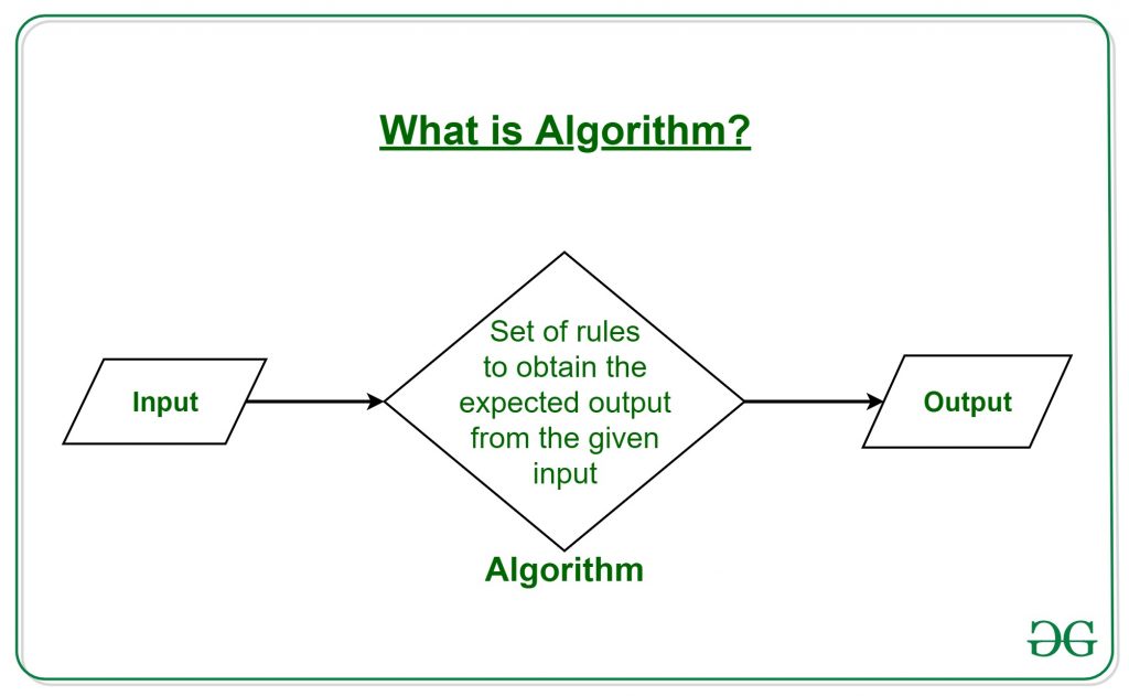
It can be understood by taking the example of cooking a new recipe. To cook a new recipe, one reads the instructions and steps and executes them one by one, in the given sequence. The result thus obtained is the new dish is cooked perfectly. Every time you use your phone, computer, laptop, or calculator you are using Algorithms. Similarly, algorithms help to do a task in programming to get the expected output.
The Algorithm designed are language-independent, i.e. they are just plain instructions that can be implemented in any language, and yet the output will be the same, as expected.
What is the need for algorithms:
1.Algorithms are necessary for solving complex problems efficiently and effectively.
2.They help to automate processes and make them more reliable, faster, and easier to perform.
3.Algorithms also enable computers to perform tasks that would be difficult or impossible for humans to do manually.
4.They are used in various fields such as mathematics, computer science, engineering, finance, and many others to optimize processes, analyze data, make predictions, and provide solutions to problems.
What are the Characteristics of an Algorithm?
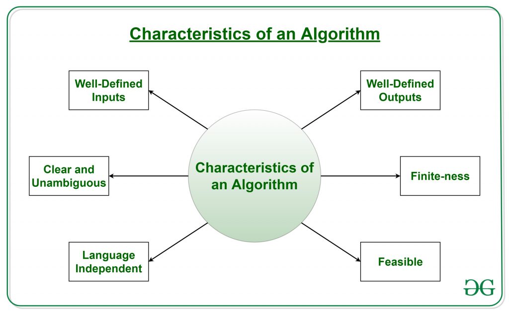
As one would not follow any written instructions to cook the recipe, but only the standard one. Similarly, not all written instructions for programming is an algorithms. In order for some instructions to be an algorithm, it must have the following characteristics:
- Clear and Unambiguous: The algorithm should be clear and unambiguous. Each of its steps should be clear in all aspects and must lead to only one meaning.
- Well-Defined Inputs: If an algorithm says to take inputs, it should be well-defined inputs. It may or may not take input.
- Well-Defined Outputs: The algorithm must clearly define what output will be yielded and it should be well-defined as well. It should produce at least 1 output.
- Finite-ness: The algorithm must be finite, i.e. it should terminate after a finite time.
- Feasible: The algorithm must be simple, generic, and practical, such that it can be executed with the available resources. It must not contain some future technology or anything.
- Language Independent: The Algorithm designed must be language-independent, i.e. it must be just plain instructions that can be implemented in any language, and yet the output will be the same, as expected.
- Input: An algorithm has zero or more inputs. Each that contains a fundamental operator must accept zero or more inputs.
- Output: An algorithm produces at least one output.Every instruction that contains a fundamental operator must accept zero or more inputs.
- Definiteness: All instructions in an algorithm must be unambiguous, precise, and easy to interpret. By referring to any of the instructions in an algorithm one can clearly understand what is to be done. Every fundamental operator in instruction must be defined without any ambiguity.
- Finiteness: An algorithm must terminate after a finite number of steps in all test cases. Every instruction which contains a fundamental operator must be terminated within a finite amount of time. Infinite loops or recursive functions without base conditions do not possess finiteness.
- Effectiveness: An algorithm must be developed by using very basic, simple, and feasible operations so that one can trace it out by using just paper and pencil.
Properties of Algorithm:
- It should terminate after a finite time.
- It should produce at least one output.
- It should take zero or more input.
- It should be deterministic means giving the same output for the same input case.
- Every step in the algorithm must be effective i.e. every step should do some work.
Types of Algorithms:
There are several types of algorithms available. Some important algorithms are:
1. Brute Force Algorithm: It is the simplest approach for a problem. A brute force algorithm is the first approach that comes to finding when we see a problem.
2. Recursive Algorithm: A recursive algorithm is based on recursion. In this case, a problem is broken into several sub-parts and called the same function again and again.
3. Backtracking Algorithm: The backtracking algorithm basically builds the solution by searching among all possible solutions. Using this algorithm, we keep on building the solution following criteria. Whenever a solution fails we trace back to the failure point and build on the next solution and continue this process till we find the solution or all possible solutions are looked after.
4. Searching Algorithm: Searching algorithms are the ones that are used for searching elements or groups of elements from a particular data structure. They can be of different types based on their approach or the data structure in which the element should be found.
5. Sorting Algorithm: Sorting is arranging a group of data in a particular manner according to the requirement. The algorithms which help in performing this function are called sorting algorithms. Generally sorting algorithms are used to sort groups of data in an increasing or decreasing manner.
6. Hashing Algorithm: Hashing algorithms work similarly to the searching algorithm. But they contain an index with a key ID. In hashing, a key is assigned to specific data.
7. Divide and Conquer Algorithm: This algorithm breaks a problem into sub-problems, solves a single sub-problem and merges the solutions together to get the final solution. It consists of the following three steps:
- Divide
- Solve
- Combine
8. Greedy Algorithm: In this type of algorithm the solution is built part by part. The solution of the next part is built based on the immediate benefit of the next part. The one solution giving the most benefit will be chosen as the solution for the next part.
9. Dynamic Programming Algorithm: This algorithm uses the concept of using the already found solution to avoid repetitive calculation of the same part of the problem. It divides the problem into smaller overlapping subproblems and solves them.
10. Randomized Algorithm: In the randomized algorithm we use a random number so it gives immediate benefit. The random number helps in deciding the expected outcome.
To learn more about the types of algorithms refer to the article about “Types of Algorithms“.
Advantages of Algorithms:
- It is easy to understand.
- An algorithm is a step-wise representation of a solution to a given problem.
- In Algorithm the problem is broken down into smaller pieces or steps hence, it is easier for the programmer to convert it into an actual program.
Disadvantages of Algorithms:
- Writing an algorithm takes a long time so it is time-consuming.
- Understanding complex logic through algorithms can be very difficult.
- Branching and Looping statements are difficult to show in Algorithms(imp).
How to Design an Algorithm?
In order to write an algorithm, the following things are needed as a pre-requisite:
- The problem that is to be solved by this algorithm i.e. clear problem definition.
- The constraints of the problem must be considered while solving the problem.
- The input to be taken to solve the problem.
- The output to be expected when the problem is solved.
- The solution to this problem, is within the given constraints.
Then the algorithm is written with the help of the above parameters such that it solves the problem.
Example: Consider the example to add three numbers and print the sum.
- Step 1: Fulfilling the pre-requisites
As discussed above, in order to write an algorithm, its pre-requisites must be fulfilled.- The problem that is to be solved by this algorithm: Add 3 numbers and print their sum.
- The constraints of the problem that must be considered while solving the problem: The numbers must contain only digits and no other characters.
- The input to be taken to solve the problem: The three numbers to be added.
- The output to be expected when the problem is solved: The sum of the three numbers taken as the input i.e. a single integer value.
- The solution to this problem, in the given constraints: The solution consists of adding the 3 numbers. It can be done with the help of ‘+’ operator, or bit-wise, or any other method.
- Step 2: Designing the algorithm
Now let’s design the algorithm with the help of the above pre-requisites:
Algorithm to add 3 numbers and print their sum:- START
- Declare 3 integer variables num1, num2 and num3.
- Take the three numbers, to be added, as inputs in variables num1, num2, and num3 respectively.
- Declare an integer variable sum to store the resultant sum of the 3 numbers.
- Add the 3 numbers and store the result in the variable sum.
- Print the value of the variable sum
- END
- Step 3: Testing the algorithm by implementing it.
In order to test the algorithm, let’s implement it in C language.
Program:
C++
#include <bits/stdc++.h>
using namespace std;
int main()
{
int num1, num2, num3;
int sum;
cout << "Enter the 1st number: ";
cin >> num1;
cout << " " << num1 << endl;
cout << "Enter the 2nd number: ";
cin >> num2;
cout << " " << num2 << endl;
cout << "Enter the 3rd number: ";
cin >> num3;
cout << " " << num3;
sum = num1 + num2 + num3;
cout << "nSum of the 3 numbers is: "
<< sum;
return 0;
}
C
#include <stdio.h>
int main()
{
int num1, num2, num3;
int sum;
printf("Enter the 1st number: ");
scanf("%d", &num1);
printf("%dn", num1);
printf("Enter the 2nd number: ");
scanf("%d", &num2);
printf("%dn", num2);
printf("Enter the 3rd number: ");
scanf("%d", &num3);
printf("%dn", num3);
sum = num1 + num2 + num3;
printf("nSum of the 3 numbers is: %d", sum);
return 0;
}
Java
import java.util.*;
class GFG {
public static void main(String[] args)
{
int sum = 0;
Scanner sc
= new Scanner(System.in);
System.out.println("Enter the 1st number: ");
int num1 = sc.nextInt();
System.out.println(" " + num1);
System.out.println("Enter the 2nd number: ");
int num2 = sc.nextInt();
System.out.println(" " + num2);
System.out.println("Enter the 3rd number: ");
int num3 = sc.nextInt();
System.out.println(" " + num3);
sum = num1 + num2 + num3;
System.out.println("Sum of the 3 numbers is = "
+ sum);
}
}
Python3
if __name__ == "__main__":
num1 = num2 = num3 = 0
sum = 0
num1 = int(input("Enter the 1st number: "))
num2 = int(input("Enter the 2nd number: "))
num3 = int(input("Enter the 3rd number: "))
sum = num1 + num2 + num3
print("nSum of the 3 numbers is:", sum)
C#
using System;
class GFG {
static public void Main ()
{
int sum = 0;
Console.Write("Enter the 1st number: ");
int num1 = int.Parse(Console.ReadLine());
Console.WriteLine(" " + num1);
Console.Write("Enter the 2nd number: ");
int num2 = int.Parse(Console.ReadLine());
Console.WriteLine(" " + num2);
Console.Write("Enter the 3rd number: ");
int num3 = int.Parse(Console.ReadLine());
Console.WriteLine(" " + num3);
sum = num1 + num2 + num3;
Console.WriteLine("Sum of the 3 numbers is = "
+ sum);
}
}
Javascript
let num1 = 0, num2 = 0, num3 = 0;
let sum = 0;
console.log("Enter the 1st number: ");
num1 = parseInt(prompt());
console.log(" " + num1 + "<br>");
console.log("Enter the 2nd number: ");
num2=parseInt(prompt());
console.log(" " + num2 + "<br>");
console.log("Enter the 3rd number: ");
num3=parseInt(prompt());
console.log(" " + num3);
sum = num1 + num2 + num3;
console.log("<br>Sum of the 3 numbers is: " + sum);
Output
Enter the 1st number: 0
Enter the 2nd number: 0
Enter the 3rd number: -1577141152

Sum of the 3 numbers is: -1577141152
Here is the step-by-step algorithm of the code:
- Declare three variables num1, num2, and num3 to store the three numbers to be added.
- Declare a variable sum to store the sum of the three numbers.
- Use the cout statement to prompt the user to enter the first number.
- Use the cin statement to read the first number and store it in num1.
- Use the cout statement to prompt the user to enter the second number.
- Use the cin statement to read the second number and store it in num2.
- Use the cout statement to prompt the user to enter the third number.
- Use the cin statement to read the third number and store it in num3.
- Calculate the sum of the three numbers using the + operator and store it in the sum variable.
- Use the cout statement to print the sum of the three numbers.
- The main function returns 0, which indicates successful execution of the program.
Time complexity: O(1)
Auxiliary Space: O(1)
One problem, many solutions: The solution to an algorithm can be or cannot be more than one. It means that while implementing the algorithm, there can be more than one method to implement it. For example, in the above problem to add 3 numbers, the sum can be calculated in many ways like:
- + operator
- Bit-wise operators
- . . etc
How to analyze an Algorithm?
For a standard algorithm to be good, it must be efficient. Hence the efficiency of an algorithm must be checked and maintained. It can be in two stages:
- Priori Analysis: “Priori” means “before”. Hence Priori analysis means checking the algorithm before its implementation. In this, the algorithm is checked when it is written in the form of theoretical steps. This Efficiency of an algorithm is measured by assuming that all other factors, for example, processor speed, are constant and have no effect on the implementation. This is done usually by the algorithm designer. This analysis is independent of the type of hardware and language of the compiler. It gives the approximate answers for the complexity of the program.
- Posterior Analysis: “Posterior” means “after”. Hence Posterior analysis means checking the algorithm after its implementation. In this, the algorithm is checked by implementing it in any programming language and executing it. This analysis helps to get the actual and real analysis report about correctness(for every possible input/s if it shows/returns correct output or not), space required, time consumed etc. That is, it is dependent on the language of the compiler and the type of hardware used.
What is Algorithm complexity and how to find it?
An algorithm is defined as complex based on the amount of Space and Time it consumes. Hence the Complexity of an algorithm refers to the measure of the Time that it will need to execute and get the expected output, and the Space it will need to store all the data (input, temporary data and output). Hence these two factors define the efficiency of an algorithm.
The two factors of Algorithm Complexity are:
- Time Factor: Time is measured by counting the number of key operations such as comparisons in the sorting algorithm.
- Space Factor: Space is measured by counting the maximum memory space required by the algorithm to run/execute.
Therefore the complexity of an algorithm can be divided into two types:
1. Space Complexity: The space complexity of an algorithm refers to the amount of memory required by the algorithm to store the variables and get the result. This can be for inputs, temporary operations, or outputs.
How to calculate Space Complexity?
The space complexity of an algorithm is calculated by determining the following 2 components:
- Fixed Part: This refers to the space that is definitely required by the algorithm. For example, input variables, output variables, program size, etc.
- Variable Part: This refers to the space that can be different based on the implementation of the algorithm. For example, temporary variables, dynamic memory allocation, recursion stack space, etc.
Therefore Space complexity S(P) of any algorithm P is S(P) = C + SP(I), where C is the fixed part and S(I) is the variable part of the algorithm, which depends on instance characteristic I.
Example: Consider the below algorithm for Linear Search
Step 1: START
Step 2: Get n elements of the array in arr and the number to be searched in x
Step 3: Start from the leftmost element of arr[] and one by one compare x with each element of arr[]
Step 4: If x matches with an element, Print True.
Step 5: If x doesn’t match with any of the elements, Print False.
Step 6: END
Here, There are 2 variables arr[], and x, where the arr[] is the variable part of n elements and x is the fixed part. Hence S(P) = 1+n. So, the space complexity depends on n(number of elements). Now, space depends on data types of given variables and constant types and it will be multiplied accordingly.
2. Time Complexity: The time complexity of an algorithm refers to the amount of time that is required by the algorithm to execute and get the result. This can be for normal operations, conditional if-else statements, loop statements, etc.
How to calculate Time Complexity?
The time complexity of an algorithm is also calculated by determining the following 2 components:
- Constant time part: Any instruction that is executed just once comes in this part. For example, input, output, if-else, switch, arithmetic operations etc.
- Variable Time Part: Any instruction that is executed more than once, say n times, comes in this part. For example, loops, recursion, etc.
Therefore Time complexity of any algorithm P is T(P) = C + TP(I), where C is the constant time part and TP(I) is the variable part of the algorithm, which depends on the instance characteristic I.
 of any algorithm P is T(P) = C + TP(I), where C is the constant time part and TP(I) is the variable part of the algorithm, which depends on the instance characteristic I.
Example: In the algorithm of Linear Search above, the time complexity is calculated as follows:
Step 1: –Constant Time
Step 2: — Variable Time (Taking n inputs)
Step 3: –Variable Time (Till the length of the Array (n) or the index of the found element)
Step 4: –Constant Time
Step 5: –Constant Time
Step 6: –Constant Time
Hence, T(P) = 5 + n, which can be said as T(n).
How to express an Algorithm?
- Natural Language :- Here we express the Algorithm in natural English language. It is too hard to understand the algorithm from it.
- Flow Chat :- Here we express the Algorithm by making graphical/pictorial representation of it. It is easier to understand than Natural Language.
- Pseudo Code :- Here we express the Algorithm in the form of annotations and informative text written in plain English which is very much similar to the real code but as it has no syntax like any of the programming language, it can’t be compiled or interpreted by the computer. It is the best way to express an algorithm because it can be understood by even a layman with some school level programming knowledge.
: a procedure for solving a mathematical problem (as of finding the greatest common divisor) in a finite number of steps that frequently involves repetition of an operation
broadly
: a step-by-step procedure for solving a problem or accomplishing some end
There are several search engines, with Google, Yahoo and Bing being the biggest players. Each search engine has its own proprietary computation (called an «algorithm«) that ranks websites for each keyword or combination of keywords. — Julie Brinton
… sometimes you solve a problem by coming up with an algorithm of some kind. But sometimes you solve a problem in a very ad hoc sort of way. —William H. Huggins

![]()
Did you know?
The current term of choice for a problem-solving procedure, algorithm, is commonly used nowadays for the set of rules a machine (and especially a computer) follows to achieve a particular goal. It does not always apply to computer-mediated activity, however. The term may as accurately be used of the steps followed in making a pizza or solving a Rubik’s Cube as for computer-powered data analysis.
Algorithm is often paired with words specifying the activity for which a set of rules have been designed. A search algorithm, for example, is a procedure that determines what kind of information is retrieved from a large mass of data. An encryption algorithm is a set of rules by which information or messages are encoded so that unauthorized persons cannot read them.
Though first attested in the early 20th century (and, until recently, used strictly as a term of mathematics and computing), algorithm has a surprisingly deep history. It was formed from algorism “the system of Arabic numerals,” a word that goes back to Middle English and ultimately stems from the name of a 9th-century Persian mathematician, abu-Jaʽfar Mohammed ibn-Mūsa al-Khuwārizmi, who did important work in the fields of algebra and numeric systems.
Example Sentences
Recent Examples on the Web
For all the excitement around ChatGPT and its ilk, the makers of today’s large language models haven’t solved the problem of biased data sets that have already embedded racist assumptions into AI applications such as face recognition and criminal risk-assessment algorithms.
—Will Oremus, Washington Post, 4 Apr. 2023
These days, many police departments use surveillance cameras and facial recognition algorithms to locate suspects.
—Annalee Newitz, Popular Mechanics, 4 Apr. 2023
ChatGPT is a machine learning model that uses statistical patterns and algorithms to generate responses to natural language inputs.
—Karen Weintraub, USA TODAY, 1 Apr. 2023
And that required, in some ways, freeing it from the bloodless grip of data analytics and algorithms that Epstein helped pioneer.
—David Axelrod, CNN, 1 Apr. 2023
Israeli hacking software, American investigation tools and Chinese computer vision algorithms can all be bought and mixed together to make a snooping cocktail of startling effectiveness.
—Adam Satariano, New York Times, 30 Mar. 2023
The members of Fall Out Boy are weighing in on the impacts of AI and algorithms on the music industry.
—Abbey White, The Hollywood Reporter, 30 Mar. 2023
Most agree that tubes in general have a sound that transistors, circuit boards, and algorithms can only approximate, one often described as warm, rich, or even romantic.
—Roy Furchgott, WIRED, 28 Mar. 2023
Additionally, different lenders may offer different loan terms based on their unique requirements and algorithms.
—Elizabeth Rivelli, Car and Driver, 27 Mar. 2023
See More
These examples are programmatically compiled from various online sources to illustrate current usage of the word ‘algorithm.’ Any opinions expressed in the examples do not represent those of Merriam-Webster or its editors. Send us feedback about these examples.
Word History
Etymology
alteration of Middle English algorisme, from Old French & Medieval Latin; Old French, from Medieval Latin algorismus, from Arabic al-khuwārizmi, from al-Khwārizmī flourished a.d. 825 Islamic mathematician
First Known Use
1926, in the meaning defined above
Time Traveler
The first known use of algorithm was
in 1926
Dictionary Entries Near algorithm
Cite this Entry
“Algorithm.” Merriam-Webster.com Dictionary, Merriam-Webster, https://www.merriam-webster.com/dictionary/algorithm. Accessed 14 Apr. 2023.
Share
More from Merriam-Webster on algorithm
Last Updated:
10 Apr 2023
— Updated example sentences
Subscribe to America’s largest dictionary and get thousands more definitions and advanced search—ad free!
Merriam-Webster unabridged
What Does Algorithm Mean?
In its purest sense, an algorithm is a mathematical process to solve a problem using a finite number of steps.
In the world of computers, an algorithm is the set of instructions that defines not just what needs to be done but how to do it.
Techopedia Explains Algorithm
Probably the best way to understand an algorithm is to think of it as a recipe. There are many ways to bake cookies, but by following a recipe a baker knows to first preheat the oven, then measure out the flour, add butter, chocolate chips, etc. until the desired cookies are complete.
Using algorithms, a programmer or computer scientist can tell his machine to query database A for last month’s sales figures, compare them to the prior month and the same month last year, and then display it in a bar graph.
Mix multiple algorithms together and you have a working computer program.
As can be expected, there are numerous types of algorithms for virtually every kind of mathematical problem there is to solve. There are:
-
Numerical algorithms.
-
Algebraic algorithms.
-
Geometric algorithms.
-
Sequential algorithms.
-
Operational algorithms.
-
Theoretical algorithms.
There are also various algorithms named after the leading mathematicians who invented them:
-
Shor’s algorithm.
-
Girvan-Newman algorithm.
-
Several Euclidian algorithms.
There are also those named after the specific problem they solve, such as:
-
Bidirectional search algorithm.
-
K-way merge algorithm.
In the computing field, most algorithms tend to solve data management and analysis problems.
Top Computing Algorithms
(According to Ohio State University)
Sort
Arranging data in an efficient and useful manner. These include quick sort, merge sort, counting sort and others;
Search
Finding key data in sorted data sets. Binary Search is used for searching in linear data structures and sorted data sets. Depth/Breadth First Search (DFS/BFS) is used for Graph data structures and is employed by search engines for web crawling.
Hashing
Similar to search but with an indexing and key ID component. Hashing provides superior results because it assigns a key to certain data;
Dynamic Programming
Converts larger, complex problems into series of smaller problems;
Exponential by Squaring (EbS)
Also known as binary exponentiation, EbS speeds up the calculation of large integers, polynomials, square matrices and other complex problems;
String Matching and Parsing
Designed to find patterns in large data sets using predefined terms and restrictions;
Primality Testing
Determines prime numbers either deterministically or probabilistically; mostly used in cryptography.
Networking also relies heavily on algorithms, which govern everything from packet routing and traffic management to security and encryption. Traditionally, routing algorithms were largely static in that they established fixed points of network activity.
Recently, however, network providers have shifted toward more adaptive algorithms that can make changes on the fly in response to traffic or topology considerations.
Algorithms are at the heart of just about everything in the digital world, from high-speed stock trading to automated dishwashers.
As technology becomes even more ubiquitous and we find ourselves relying on smart cars, smart homes, smart cities and even smart bodies, it may seem like we are interacting with an entirely new form of consciousness on the planet, one that walks, talks and thinks.
In reality, though, it’s just lots of numbers running through lots of algorithms.
In mathematics and computing, an algorithm is a finite sequence of well-defined instructions for accomplishing some task that, given an initial state, will terminate in a defined end-state. Informally, the concept of an algorithm is often illustrated by the example of a recipe, albeit more complex. Algorithms often contain steps that repeat (iterate) or require decisions, such as by using logic or comparisons.
Algorithms constitute a foundational concept in computer science. In most higher-level computer programs, algorithms act in complex patterns, each using smaller and smaller sub-methods, which are built up to the program as a whole. In other words, a computer program may be regarded as an algorithm that has nested sets of smaller algorithms within it. Most algorithms can be directly implemented by computer programs; any other algorithms can at least in theory be simulated by computer programs.
History
As early as 1600 B.C.E., the Babylonians developed algorithms for factorization and finding square roots of numbers. The Euclidean algorithm, given in Euclid’s Elements around 300 B.C.E., was useful for determining the greatest common divisor of two integers, among other things. The latter algorithm was probably not discovered by Euclid and may have been known by the Greeks up to 200 years earlier.
Between CE 813 and 833, Persian mathematician Al-Khawarizmi (Abu Ja’afar Abdullah Muhammad Ibn Mūsā al-Khawārizmī) described a procedure for solving linear equations and quadratic equations. The word «algorithm,» used for such a procedure, comes from his name.
Initially, the term «algorism» was used to refer to the rules of performing arithmetic computations with Hindu-Arabic numerals. Later, based on European Latin translations of al-Khwarizmi’s name, the word evolved into «algoritmi» and then «algorithm» by the eighteenth century. The meaning of the word was also broadened to include all definite mathematical procedures for solving problems or performing tasks.
The lack of mathematical rigor in the «well-defined procedure» definition of algorithms posed some difficulties for mathematicians and logicians of the nineteenth and early twentieth centuries. Their understanding of algorithms, however, was greatly improved in 1936, with Alan Turing’s description of the «Turing machine» (an abstract model of a computer), and the assertion that all possible calculations can be emulated on a Turing machine—a statement known as the «Church-Turing thesis,» which has so far not been contradicted. Currently, a formal criterion for an algorithm is that it is a procedure that can be implemented on a completely specified Turing machine or equivalent formalism. In this manner, the concept of an algorithm has become a foundation for the development of computer science.
The first case of an algorithm written for a computer occurs in Ada Lovelace’s notes on Charles Babbage’s analytical engine, written in 1842. For that, she is considered by many to be the world’s first programmer. Babbage, however, never completed his analytical engine, and the algorithm was never implemented on it.
Formalization of algorithms
Algorithms are essential to the way computers process information. A computer program is basically an algorithm that tells the computer what specific steps to perform, and in what order, to carry out a specified task. The task could be something like calculating employees’ paychecks or printing students’ report cards. In formal terms, an algorithm can be considered to be any sequence of operations that can be performed by a «Turing-complete» system—that is, a programming language that has a computational power equivalent to a universal Turing machine.
Typically, when an algorithm is associated with processing information, data is read from an input source or device, written to an output sink or device, and stored for further processing. Such data is stored in a data structure (a tool for efficiently storing data in a computer), and a predefined set of operations may be performed on it based on the demands of the algorithm.
For any such computational process, an algorithm must be rigorously defined—that is, specified in a way that applies to all possible circumstances. In other words, it must be able to deal with any possible discrepancy, error, or alternative situation occurring during the computation. For example, it needs to be able to deal with an invalid input, such as a letter instead of a number.
Algorithms generally execute their operations in sequential order: From top to bottom, and left to right. Occasionally, however, certain control structures (such as loops) can alter the order in which a particular segment of the program is conducted.
A computer program may be regarded as an algorithm that has a set of smaller algorithms within it, and each of these may contain additional subsets of algorithms. This design is called «top-down design,» where each level of abstraction (from the main algorithm to the sub-algorithms and so on) increases in specificity and detail. To illustrate, each sub-algorithm is designed to complete a specific task, and the main algorithm brings the results of these tasks together to generate a solution (or output) for the computational problem.
This type of formalization of an algorithm is based on the premises of «imperative programming»—a formalism that describes a task in discrete, «mechanical» terms. Unique to this concept of formalized algorithms is the «assignment operation,» setting the value of a variable. It derives from the intuition of «memory» as a scratch pad. (Alternate concepts of an algorithm can be found in «functional programming» and «logic programming.»)
Knuth’s characterization
Donald Knuth made a list of five properties that are still widely accepted as requirements for an algorithm:[1]
- Finiteness: «An algorithm must always terminate after a finite number of steps.»
- Definiteness: «Each step of an algorithm must be precisely defined; the actions to be carried out must be rigorously and unambiguously specified for each case.»
- Input: «…quantities which are given to it initially before the algorithm begins. These inputs are taken from specified sets of objects.»
- Output: «…quantities which have a specified relation to the inputs.»
- Effectiveness: «…all of the operations to be performed in the algorithm must be sufficiently basic that they can in principle be done exactly and in a finite length of time by a man using paper and pencil.»
An example of such an algorithm would be the Euclidean algorithm for determining the greatest common divisor of two natural numbers.
This description of an algorithm is intuitively clear but lacks formal rigor. Some terms—such as «precisely defined,» «rigorously and unambiguously specified,» or «sufficiently basic,»—are not exactly clear.
Thus the academically accepted definition of an algorithm stipulates a finite time frame of operation. Some, however, insist that the definition should include procedures that may run forever without stopping, arguing that some entity may be required to carry out such tasks. In such a case, the success of the algorithm needs to be redefined, to allow for output sequences that are unconstrained by time. For example, an algorithm that verifies if there are more zeros than ones in an infinite random binary sequence must run forever, to be effective. If implemented correctly, the algorithm’s output will be useful. For as long as it examines the sequence, the algorithm gives a positive response when the number of examined zeros outnumber the ones, and a negative response otherwise. Success for this algorithm could then be defined as eventually producing only positive responses if the sequence has more zeros than ones, and producing mixtures of positive and negative responses in other cases.
Expressing algorithms
Algorithms can be expressed in many types of notation, such as natural languages, pseudocode, flowcharts, and programming languages. Natural language expressions of algorithms tend to be verbose and ambiguous, and they are rarely used for complex or technical algorithms. Pseudocode and flowcharts are structured ways to express algorithms that avoid many of the ambiguities common in natural language statements, while avoiding implementation details. Programming languages are primarily intended for expressing algorithms in a form that can be executed by a computer, but they are often used as a way to define or document algorithms.
Implementation
Most algorithms are intended to be implemented as computer programs. Many algorithms, however, are implemented by other means, such as a biological neural network—the human brain implementing arithmetic or an insect relocating food—or an electric circuit, or a mechanical device.
Examples
One of the simplest algorithms is to pick out the largest number from an unsorted list of numbers. The solution necessarily requires looking at every number in the list, but only once at each. From this follows a simple algorithm, which can be stated in English as follows:
- Assume the first item is the largest.
- Look at each of the remaining items in the list, and if a particular item is larger than the largest item found so far, make a note of it.
- The last noted item is the largest in the list when the process is complete.
Here is a more formal coding of the algorithm in pseudocode:
Algorithm LargestNumber
  Input: A list of numbers L.
  Output: The largest number in the list L.
  if L.size = 0 return null
  largest ← L[0]
  for each item in L, do
    if item > largest, then
      largest ← item
  return largest
- «←» is a loose shorthand for «changes to». For instance, with «largest ← the item«, it means that the largest number found so far changes to this item.
- «return» terminates the algorithm and outputs the value listed behind it.
Below is a much simpler algorithm presented somewhat formally but still in English instead of pseudocode. It determines whether a given number n is even or odd:
- BEGIN
- Read the value of n.
- Divide n by 2 and store the remainder in rem.
- If rem is 0, go to step 7.
- Print «n is an odd number.»
- Go to step 8.
- Print «n is an even number.»
- END
A more complex example is Euclid’s algorithm, which is one of the oldest algorithms.
Algorithm analysis
As it happens, most people who implement algorithms want to know how much of a particular resource (such as time or storage) is required for a given algorithm. Methods have been developed for the analysis of algorithms to obtain such quantitative answers. For example, the above algorithm has a time requirement of O(n), using the big O notation with n as the length of the list. At all times, the algorithm needs to remember only two values: The largest number found so far, and its current position in the input list. Therefore it is said to have a space requirement of O(1) In this example the sizes of the numbers themselves could be unbounded and one could therefore argue that the space requirement is O(log n). In practice, however, the numbers considered would be bounded and hence the space taken up by each number is fixed. (Note that the size of the inputs is not counted as space used by the algorithm.)
Different algorithms may complete the same task with a different set of instructions in less or more time, space, or effort than others. For example, consider two different recipes for making a casserole: One is a frozen package and simply needs to be warmed up in the microwave; but the other spells out how to make a casserole from scratch and involves using a conventional oven. Both recipes end up with roughly the same dish, but each has a different time and space requirement.
The analysis and study of algorithms is a field within computer science and is often practiced abstractly (without the use of a specific programming language or other implementation). In this sense, it resembles other mathematical disciplines in that the analysis focuses on the underlying principles of the algorithm, not on any particular implementation. The pseudocode is simplest and abstract enough for such analysis.
Classes
There are various ways to classify algorithms, each with its own merits.
Classification by implementation
One way to classify algorithms is by implementation means.
- Recursion or iteration: A recursive algorithm is one that invokes (makes reference to) itself repeatedly until a certain condition is met, a method common to functional programming. Iterative algorithms use repetitive control structures, like loops, to solve the given problems. A programmer has to determine which method is best to use for a particular problem.
- Serial or parallel: Algorithms that are executed sequentially (one at a time) are known to be serial. Parallel algorithms take advantage of computer architectures where several processors can work on a problem at the same time. Parallel algorithms divide the problem into more symmetrical or asymmetrical sub-problems and pass them to many processors and put the results back together at the end. Problems that have no parallel algorithms are called «inherently serial problems.»
- Deterministic or random: Deterministic algorithms solve problems with exact decisions at every step of the algorithm. Randomized algorithms, as their name suggests, explore the search space randomly until an acceptable solution is found.
- Exact or approximate: While many algorithms reach an exact solution, approximation algorithms seek an approximation which is close to the true solution. Approximation may use either a deterministic or a random strategy. Such algorithms have practical value for many hard problems, usually dealing with physical situations.
Classification by design paradigm
Another way of classifying algorithms is by their design methodology or paradigm. There are a certain number of paradigms, each different from the other. Furthermore, each of these categories will include many different types of algorithms. Some commonly found paradigms include:
- A divide and conquer algorithm repeatedly reduces an instance of a problem to one or more smaller instances of the same problem (usually recursively), until the instances are small enough to solve easily. An example of such is Binary Search; given a sorted list of characters and a target character, it will check the midpoint character in the list and tests to see if it is the target character, and if not, whether the target is above or below the midpoint. Then, it uses the midpoint character as one of the bounds and then checks the new midpoint character of the one half of the list it is now searching. It repeats this procedure until the target is found or it cannot continue.
- A Dynamic programming algorithm is used when a problem requires the same task or calculation to be done repeatedly throughout the program. Removing the redundancy can optimize such a program, which is done by performing the repeated operations just once and storing the result for later use.
- A greedy algorithm is similar to a dynamic programming algorithm, but the difference is that solutions to the sub-problems do not have to be known at each stage; instead a «greedy» choice can be made of what looks best for the moment. The difference between dynamic programming and greedy method is, it extends the solution with the best possible decision (not all feasible decisions) at an algorithmic stage based on the current local optimum and the best decision (not all possible decisions) made in previous stage. It is not exhaustive, and does not give accurate answer to many problems. But when it works, it will be the fastest method.
- Linear programming. When solving a problem using linear programming, the program is put into a number of linear inequalities and then an attempt is made to maximize (or minimize) the inputs. Many problems (such as the maximum flow for directed graphs) can be stated in a linear programming way, and then be solved by a generic algorithm such as the simplex algorithm. A complex variant of linear programming is called integer programming, where the solution space is restricted to all integers.
- Reduction is another powerful technique in solving many problems by transforming one problem into another problem. For example, one selection algorithm for finding the median in an unsorted list is first translating this problem into sorting problem and finding the middle element in sorted list. The goal of reduction algorithms is finding the simplest transformation such that the complexity of the reduction algorithm does not dominate the complexity of the reduced algorithm. This technique is also called «transform and conquer.»
- Search and enumeration: Many problems (such as playing chess) can be modeled as problems on graphs. A graph exploration algorithm specifies rules for moving around a graph and is useful for such problems. This category also includes the search algorithms and backtracking.
- The probabilistic and heuristic paradigm: Algorithms belonging to this class fit the definition of an algorithm more loosely.
- Probabilistic algorithms are those that make some choices randomly (or pseudo-randomly); for some problems, it can in fact be proven that the fastest solutions must involve some randomness.
- Genetic algorithms attempt to find solutions to problems by mimicking the theory of biological evolution, in which cycles of «random mutations» are thought to yield successive generations of «solutions.» This process is likened to the concept of «survival of the fittest.» In genetic programming, the algorithm is regarded as a «solution» to a problem.
- Heuristic algorithms, whose general purpose is not to find an optimal solution, but an approximate solution where the time or resources to find a perfect solution are not practical. An example of this would be local search, taboo search, or simulated annealing algorithms, a class of heuristic probabilistic algorithms that vary the solution of a problem by a random amount.
Classification by field of study
Every field of science has its own problems and needs efficient algorithms. Related problems in one field are often studied together. Some example classes are search algorithms, sorting algorithms, merge algorithms, numerical algorithms, graph algorithms, string algorithms, computational geometric algorithms, combinatorial algorithms, machine learning, cryptography, data compression algorithms, and parsing techniques.
Some of these fields overlap with each other and advancing in algorithms for one field causes advancement in many fields and sometimes completely unrelated fields. For example, dynamic programming is originally invented for optimization in resource consumption in industries, but it is used in solving a broad range of problems in many fields.
Classification by complexity
Some algorithms complete in linear time, some complete in an exponential amount of time, and some never complete. One problem may have multiple algorithms, and some problems may have no algorithms. Some problems have no known efficient algorithms. There are also mappings from some problems to other problems. So computer scientists found it is suitable to classify the problems rather than algorithms into equivalence classes based on their complexity.
Notes
- ↑ Donald E. Knuth, The Art of Computer Programming Volume 1/Fundamental Algorithms (2nd ed.) (Addison-Wesley, 1973 ISBN 0201038099), 1-9.
References
ISBN links support NWE through referral fees
- Church, Alonzo. «An Unsolvable Problem of Elementary Number Theory» The American Journal Of Mathematics 58 (1936): 345-363.
- Davis, Martin. The Undecidable: Basic Papers On Undecidable Propositions, Unsolvable Problems and Computable Functions New York:Raven Press, 1965.
- Knuth, Donald E. The Art of Computer Programming, Volume 1/Fundamental Algorithms (2nd ed.) Addison-Wesley, 1973. ISBN 0201038099
- Post, Emil. «Finite Combinatory Processes, Formulation I» The Journal of Symbolic Logic 1 (1936): 103-105.
- Rosser, J.B. «An Informal Exposition of Proofs of Godel’s Theorem and Church’s Theorem» Journal of Symbolic Logic 4 (1939).
External links
All links retrieved May 16, 2021.
- Algorithms Everyday Mathematics
Credits
New World Encyclopedia writers and editors rewrote and completed the Wikipedia article
in accordance with New World Encyclopedia standards. This article abides by terms of the Creative Commons CC-by-sa 3.0 License (CC-by-sa), which may be used and disseminated with proper attribution. Credit is due under the terms of this license that can reference both the New World Encyclopedia contributors and the selfless volunteer contributors of the Wikimedia Foundation. To cite this article click here for a list of acceptable citing formats.The history of earlier contributions by wikipedians is accessible to researchers here:
- Algorithm history
- Timeline_of_algorithms history
- Euclidean_algorithm history
The history of this article since it was imported to New World Encyclopedia:
- History of «Algorithm»
Note: Some restrictions may apply to use of individual images which are separately licensed.
English[edit]
Alternative forms[edit]
- algorism (obsolete)
- augrim (obsolete)
Etymology[edit]
From Middle English algorisme, augrym, from Anglo-Norman algorisme, augrim, from Medieval Latin algorismus, from Arabic الخَوَارِزْمِيّ (al-ḵawārizmiyy), the nisba of Persian mathematician Muḥammad ibn Mūsā al-Khwārizmī and a toponymic name meaning «person from Chorasmia». The spelling change (-s- > -th-) was influenced by unrelated Ancient Greek ἀριθμός (arithmós) (whence English arithmo-) [1].
Pronunciation[edit]
- (Received Pronunciation) enPR: ălʹgə-rĭ-thəm, ălʹgə-rĭth-m, IPA(key): /ˈælɡəɹɪðəm/, [ˈæɫɡəɹɪðm̩]
- (General American) enPR: ălʹgə-rĭ’thəm, ălʹgə-rĭth‘m, IPA(key): /ˈælɡəˌɹɪðəm/, [ˈæɫɡəˌɹɪðm̩]
- Hyphenation UK: al‧gorithm, US: al‧go‧rithm
Noun[edit]
algorithm (countable and uncountable, plural algorithms)
- (countable) A collection of ordered steps that solve a mathematical problem. A precise step-by-step plan for a computational procedure that possibly begins with an input value and yields an output value in a finite number of steps.
- 1990, Cormen, Leiserson, and Rivest, Introduction to Algorithms: page 1. Cambridge, MA, The MIT Press, 1999 (23rd printing)
- Informally, an algorithm is any well-defined computational procedure that takes some value, or set of values, as input and produces some value, or set of values, as output. An algorithm is thus a sequence of computational steps that transform the input into the output.
-
2010, Aaron Sorkin, The Social Network:
-
Mark Zuckerberg: No, I need the algorithm you used to rank chess players. / Eduardo Saverin: Are you OK? / Mark Zuckerberg: We’re ranking girls.
-
-
2013 July 26, Leo Hickman, “How algorithms rule the world”, in The Guardian Weekly[1], volume 189, number 7, page 26:
-
The use of algorithms in policing is one example of their increasing influence on our lives. And, as their ubiquity spreads, so too does the debate around whether we should allow ourselves to become so reliant on them – and who, if anyone, is policing their use.
-
-
2018 February 26, Tad Friend, quoting Donald Glover, “Donald Glover Can’t Save You”, in The New Yorker[2]:
-
(Glover began his acceptance speech by saying, “First, I want to thank the algorithm that put us all here.”)
-
-
2018 June 25, Sam Jones, “Ex-Nato chief refused visa waiver to US because of Iran trips”, in The Guardian:
-
It’s a computer – an algorithm – and if you’ve been in Iran lately, they take you out of the system.
-
- 1990, Cormen, Leiserson, and Rivest, Introduction to Algorithms: page 1. Cambridge, MA, The MIT Press, 1999 (23rd printing)
- (uncountable, obsolete) Calculation with Arabic numerals; algorism.
Hyponyms[edit]
- approximation algorithm
- Baum-Welch algorithm
- Bellman-Ford algorithm
- Bresenham’s algorithm
- British Museum algorithm
- Buchberger’s algorithm
- checksum algorithm
- classification algorithm
- Cohen-Sutherland algorithm
- compression algorithm
- computer arithmetic algorithm
- Cooley-Tukey algorithm
- Davis-Putnam algorithm
- diamond-square algorithm
- Dijkstra’s algorithm
- distributed algorithm
- divide and conquer algorithm
- Douglas-Peucker algorithm
- Eppstein’s algorithm
- Euclidean algorithm
- Euclid’s algorithm
- extended Euclidean algorithm
- Fiduccia-Mattheyses algorithm
- Flajolet-Martin algorithm
- Floyd-Warshall algorithm
- forward-backward algorithm
- genetic algorithm
- Gibbs algorithm
- God’s algorithm
- Gosper’s algorithm
- greedy algorithm
- Grover’s algorithm
- hash algorithm
- Hopcroft’s algorithm
- Johnson’s algorithm
- Kadane’s algorithm
- Kahan summation algorithm
- Karatsuba algorithm
- Kernighan-Lin algorithm
- Knuth-Bendix completion algorithm
- Knuth-Morris-Pratt algorithm
- Kociemba’s algorithm
- Korf’s algorithm
- Lanczos algorithm
- Las Vegas algorithm
- Lee algorithm
- Luhn algorithm
- memetic algorithm
- Metropolis-Hastings algorithm
- Nagle’s algorithm
- painter’s algorithm
- parallel algorithm
- Peterson’s algorithm
- Pollard’s rho algorithm
- Quine-McCluskey algorithm
- Ramer-Douglas-Peucker algorithm
- randomized algorithm
- Reingold-Tilford algorithm
- Remez algorithm
- Rete algorithm
- Sattolo’s algorithm
- Schensted algorithm
- Schönhage-Strassen algorithm
- semi-algorithm
- sequential algorithm
- Shor’s algorithm
- shunting-yard algorithm
- SMAWK algorithm
- spigot algorithm
- Strassen algorithm
- Suurballe’s algorithm
- Thistlethwaite’s algorithm
- Toom-Cook algorithm
- Viterbi algorithm
- wake-sleep algorithm
- Warnock algorithm
- Warnock’s algorithm
- ziggurat algorithm
[edit]
Descendants[edit]
- → Japanese: アルゴリズム (arugorizumu)
- → Korean: 알고리즘 (algorijeum)
Translations[edit]
well-defined procedure
- Albanian: algoritëm m
- Arabic: خُوَارِزْمِيَّة f (ḵuwārizmiyya)
- Aragonese: algorismo m
- Aramaic:
- Syriac: ܚܘܪܙܐ m
- Armenian: ալգորիթմ (hy) (algoritʿm)
- Asturian: algoritmu m
- Azerbaijani: alqoritm (az)
- Belarusian: алгары́тм m (alharýtm), альгары́тм m (alʹharýtm)
- Bengali: অ্যালগরিদম (êlgōridom)
- Breton: algoritm (br) m, treol (br) m
- Bulgarian: алгори́тъм (bg) m (algorítǎm)
- Catalan: algorisme (ca) m
- Chinese:
- Mandarin: 算法 (zh) (suànfǎ), 演算法 (yǎnsuànfǎ)
- Czech: algoritmus (cs) m
- Danish: algoritme (da) c
- Dutch: algoritme (nl) n
- Esperanto: algoritmo (eo)
- Estonian: algoritm (et)
- Finnish: algoritmi (fi)
- French: algorithme (fr) m
- Galician: algoritmo (gl) m
- Georgian: ალგორითმი (ka) (algoritmi)
- German: Algorithmus (de) m
- Greek: αλγόριθμος (el) m (algórithmos)
- Hebrew: אַלגוֹרִיתְם (he) m (algorítem)
- Hindi: अल्गोरिद्म (algoridma)
- Hungarian: algoritmus (hu)
- Icelandic: reiknirit n, algrím n, reiknisögn f, algóriþmi m
- Ido: algoritmo (io)
- Indonesian: algoritme (id)
- Interlingua: algorithmo
- Italian: algoritmo (it) m
- Japanese: アルゴリズム (ja) (arugorizumu), 演算手順 (えんざんてじゅん, enzantejun), 算法 (さんぽう, sanpō) (archaic)
- Kazakh: алгоритм (kk) (algoritm)
- Korean: 알고리즘 (ko) (algorijeum), 알고리듬 (ko) (algorideum), 산법(算法) (sanbeop)
- Kyrgyz: алгоритм (algoritm)
- Lao: ຂັ້ນຕອນວິທີ (lo) (khan tǭn wi thī)
- Latin: algorithmus m
- Latvian: algoritms m
- Lithuanian: algoritmas (lt) m
- Macedonian: алгори́там m (algorítam)
- Malay: algoritma, alkhwarizmi
- Maori: hātepe, hātepe papatono
- Mirandese: algoritmo m
- Mongolian:
- Cyrillic: алгоритм (mn) (algoritm)
- Norwegian:
- Bokmål: algoritme (no) m
- Occitan: algoritme (oc) m
- Persian: الگوریتم (fa) (algoritm)
- Polish: algorytm (pl) m
- Portuguese: algoritmo (pt) m
- Romanian: algoritm (ro) m
- Russian: алгори́тм (ru) m (algorítm)
- Scots: algorithm
- Serbo-Croatian:
- Cyrillic: алгорѝтам m
- Roman: algorìtam m
- Slovak: algoritmus m
- Slovene: algoritem m
- Spanish: algoritmo (es) m
- Swedish: algoritm (sv) c
- Tagalog: algorítmo
- Tajik: алгоритм (tg) (algoritm)
- Thai: อัลกอริทึม (an-gɔɔ-rí-tʉ̂m), ขั้นตอนวิธี (kân-dtɔɔn-wí-tii)
- Turkish: algoritma (tr)
- Turkmen: algoritm
- Ukrainian: алгори́тм (uk) m (alhorýtm)
- Uzbek: algoritm (uz)
- Vietnamese: thuật toán (vi)
- Yiddish: אַלגאָריטם m (algoritm)
See also[edit]
- data structure
- function
- program
References[edit]
- ^ Knuth, Donald (1997). «The Art of Computer Programming, Volume 1, 3rd ed. Addison-Wesley, page 1. →ISBN.
Anagrams[edit]
- logarithm, mithralog
You may remember your math teacher from grade school asking for an answer to a question using a specific algorithm, but do you know what the word algorithm means? We’ll tell you!
In this guide, we explore the term algorithm to uncover its definition, origin, synonyms, antonyms, and more.

What Is the Definition of Algorithm?
Cambridge Dictionary defines algorithm as a set of mathematical rules or instructions that will help to obtain the answer to a problem (especially used in computing). One example is music apps like Pandora and Spotify use algorithms to predict the next song played based on past songs played and artists you may have liked or disliked along the way.
Basically, an algorithm is a set of step-by-step procedures that will solve a particular problem or task if followed correctly. We encounter algorithms every day, and we may not even notice them. From the recipe you used to bake your favorite cake last week to the everyday use of Google and other search engines, these are all algorithms (or examples of them).
What Are the Types of Algorithms?
Since algorithms are a set of rules used to solve a task or issue, there are many types of algorithms — with the most common type being computer science algorithms.
In computer science, a coder creates a set of codes that artificial intelligence (or a computer) uses to solve problems. Below, we have compiled a shortlist of the different types of computer science algorithms.
Study these to help you get better acquainted with all the varying types of algorithms you may encounter:
- Backtracking algorithms
- Divide and conquer algorithms
- Recursive algorithms
- Dynamic programming algorithms
- Greedy algorithms
- Brute force algorithms
- Randomized algorithms
What Is the Etymology of Algorithm?
Do you remember the childhood game “telephone?” Well, the etymology behind our word of the day is best described as a game of telephone gone poorly.
The origin of algorithm begins in the ninth century when a Persian mathematician at the Royal Court in Baghdad named Mohammed ibn-Musa al-Khwarizmi wrote about calculations and Hindu-Arabic numerals. Later his work was translated into Latin — and with this, the game is afoot.
As Al-Khwarizmi’s work was translated into Latin, his name was then integrated into the process he wrote, forming the Medieval Latin algorismus. From there Al-Khwārizmī’s name was Latinized as Algoritmi. This Latinized name of the this Persian mathematician is where the game of telephone starts to get a little off track, so to speak.
The name algoritmi was mixed up with the Ancient Greek word for numbers, arithmos. Over time this confusion led to the evolution of the word algorithm as we currently use it today.
Through the mistaken connection with Greek arithmos, the Old French word for the Arabic numeral system (algorisme) was refashioned into the French algorithme. You may have guessed that the word, algorithm, is a derivative of the French algorithme.
What Are the Synonyms and Antonyms of Algorithm?
By now, you know that the word algorithm refers to a set of rules for solving a problem in a finite number of steps. To further your overall understanding of the term, we’ve compiled a list of synonyms and antonyms for you to review.
Here are a few synonyms provided by Power Thesaurus:
- Computation
- Method
- Set of rules
- Algorithmic program
- System
- Script
- Computer program
- Subroutine
- Mathematical problem
- Process
- Algorithmic rule
- Algorithm
- Form
- Set of instructions
- Discovery
- Calculation
- Functions
The antonyms of algorithm include:
- Misconception
- Yang
- Yin
- Loss
- Miss
How Can You Use Algorithm in a Sentence?
One of the top ways we can commit new knowledge to memory is by using it in everyday communication. From text messages with friends to written papers for work, test your new knowledge and push yourself by incorporating algorithm into sentences today.
Below you will find a few example sentences to help get you started:
Mark, we are not looking for you to employ heuristics with this. What we need is an algorithm in place to get this done correctly the first time.
What algorithm did you use to answer question 14 on the quiz in computer science?
If you like learning computer algorithms, you may want to consider a career in IT.
The standard algorithm for subdivision can be found in your textbook on page 68.
We had to provide an example of an algorithm before leaving class today.
Today, we learned about the Euclidean algorithm and how it is used to find the greatest common divisor.
The tech company uses machine learning algorithms to recommend open positions to those looking for a good job.
Conclusion
In short, an algorithm will always include a finite set of steps that you can use to solve any problem. From simple division to the step-by-step method of how to solve a Rubix cube, varying algorithms are around us at all times.
Sources:
- Algorithm | Cambridge English Dictionary
- Algorithm synonyms 172 Words and Phrases for Algorithm | Power Thesaurus
- Algorithm definition and meaning | Collins English Dictionary

Kevin Miller is a growth marketer with an extensive background in Search Engine Optimization, paid acquisition and email marketing. He is also an online editor and writer based out of Los Angeles, CA. He studied at Georgetown University, worked at Google and became infatuated with English Grammar and for years has been diving into the language, demystifying the do’s and don’ts for all who share the same passion! He can be found online here.
What is an algorithm?
An algorithm is a procedure used for solving a problem or performing a computation. Algorithms act as an exact list of instructions that conduct specified actions step by step in either hardware- or software-based routines.
Algorithms are widely used throughout all areas of IT. In mathematics and computer science, an algorithm usually refers to a small procedure that solves a recurrent problem. Algorithms are also used as specifications for performing data processing and play a major role in automated systems.
An algorithm could be used for sorting sets of numbers or for more complicated tasks, like recommending user content on social media. Algorithms typically start with initial input and instructions that describe a specific computation. When the computation is executed, the process produces an output.
How do algorithms work?
Algorithms can be expressed as natural languages, programming languages, pseudocode, flowcharts and control tables. Natural language expressions are rare, as they are more ambiguous. Programming languages are normally used for expressing algorithms executed by a computer.
Algorithms use an initial input along with a set of instructions. The input is the initial data needed to make decisions and can be represented in the form of numbers or words. The input data gets put through a set of instructions, or computations, which can include arithmetic and decision-making processes. The output is the last step in an algorithm and is normally expressed as more data.
For example, a search algorithm takes a search query as input and runs it through a set of instructions for searching through a database for relevant items to the query. Automation software acts as another example of algorithms, as automation follows a set of rules to complete tasks. Many algorithms make up automation software, and they all work to automate a given process.
What are different types of algorithms?
There are several types of algorithms, all designed to accomplish different tasks. For example, algorithms perform the following:
- Search engine algorithm. This algorithm takes search stringsof keywords and operators as input, searches its associated database for relevant webpages and returns results.
- Encryption algorithm. This computing algorithm transforms data according to specified actions to protect it. A symmetric key algorithm, such as the Data Encryption Standard, for example, uses the same keyto encrypt and decrypt data. As long as the algorithm is sufficiently sophisticated, no one lacking the key can decrypt the data.
- Greedy algorithm. This algorithm solves optimization problems by finding the locally optimal solution, hoping it is the optimal solution at the global level. However, it does not guarantee the most optimal solution.
- Recursive algorithm. This algorithm calls itself repeatedly until it solves a problem. Recursive algorithms call themselves with a smaller value every time a recursive function is invoked.
- Backtracking algorithm. This algorithm finds a solution to a given problem in incremental approaches and solves it one piece at a time.
- Divide-and-conquer algorithm. This common algorithm is divided into two parts. One part divides a problem into smaller subproblems. The second part solves these problems and then combines them together to produce a solution.
- Dynamic programming algorithm. This algorithm solves problems by dividing them into subproblems. The results are then stored to be applied for future corresponding problems.
- Brute-force algorithm. This algorithm iterates all possible solutions to a problem blindly, searching for one or more solutions to a function.
- Sorting algorithm. Sorting algorithms are used to rearrange data structure based on a comparison operator, which is used to decide a new order for data.
- Hashing algorithm. This algorithm takes data and converts it into a uniform message with a hashing
- Randomized algorithm. This algorithm reduces running times and time-based complexities. It uses random elements as part of its logic.
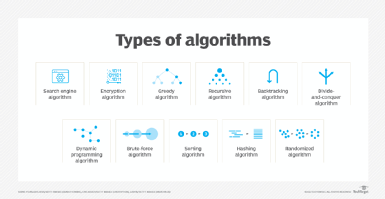
What are examples of algorithms?
Machine learning is a good example of an algorithm, as it uses multiple algorithms to predict outcomes without being explicitly programmed to do so. Machine learning uses supervised learning or unsupervised learning. In supervised learning, data scientists supply complex algorithms with labeled training data and define the variables they want the algorithm to assess for correlations. Both the input and the output of the algorithm are specified.
Unsupervised machine learning involves algorithms that train on unlabeled data. Unsupervised machine learning algorithms sift through unlabeled data to look for patterns that can be used to group data points into subsets. Most types of deep learning, including neural networks, are unsupervised algorithms.
Machine learning used in artificial intelligence also relies on algorithms. However, machine learning-based systems may have inherent biases in the data that feeds the machine learning algorithm. This could result in systems that are untrustworthy and potentially harmful.
Learn about algorithms, algorithm bias and how to combat algorithm bias.
This was last updated in May 2022
Continue Reading About algorithm
- A look at AI trends and bias in AI algorithms
- Hiring algorithms prove beneficial, but also raise ethical questions
- How Getty Images reduces bias in AI algorithms to avoid harm
- How to find the best machine learning frameworks for you
- 6 ways to reduce different types of bias in machine learning
They have very intense and high-level discussions about their work with Dad quite often, and the word algorithm features extremely heavily. ❋ Holly McQueen (2010)
The term algorithm simply means a series of steps. ❋ Unknown (2008)
I wonder if the algorithm is a little “loose” to get as many copies out as possible? — melissa ❋ Unknown (2008)
The term algorithm is derived from the name of the Arabic economist, Al-Khowërazmi, who invented them as a way of performing mathematical operations associated with debt and credit. ❋ Unknown (1997)
At Consumer Reports, we’re increasingly encountering the term algorithm in reference to smart appliances: dryers that know when loads are dry, refrigerators that can self-regulate their temperature, and dishwashers that sense when dishes are done. ❋ Unknown (2008)
As far as Digg goes, their algorithm is woefully bad at allowing folks to call things that are partisan be called inaccurate and be buried. ❋ Unknown (2009)
H. 264, currently the most efficient video compression algorithm, is also, since Adobe integrated the codec into its Flash Player, used for web videos and now Microsoft is also adding H. 264 to Silverlight 3. ❋ Unknown (2009)
In any case, an evolutionary algorithm is a model of the behavior of generalized replicators. ❋ Unknown (2010)
An evolutionary algorithm is a program, and like all programs, is independent on the substrate. ❋ Unknown (2010)
“The principal datum input to any search algorithm is a description of its search space.” ❋ Unknown (2009)
The filtering algorithm is mysterious, but you can tweak it by either clicking the little pencil that appears on the right when you hover over an item (you can specify that you would like to see more or fewer items of this type or from this user) or by clicking the «Options for News Feed» link all the way at the bottom of this page. ❋ Unknown (2009)
The really cool thing about this algorithm is that the computers in the network figure this all out themselves, without human intervention. ❋ Unknown (2010)
The most famous part of our ranking algorithm is PageRank, an algorithm developed by Larry Page and Sergey Brin, who founded Google. ❋ Unknown (2008)
Called VisualRank, the new algorithm is based on a scoring system on relevance developed by Google employees. ❋ Unknown (2008)
How did you [translate] the [data] from the hashtable to a few characters?
An algorithm.
How did you make the game run faster?
I [optimized] the running time of the algorithm. ❋ IHazABone (2015)
An example of an algorithm is how your computer works. [You tell it] what to do and it utilizes all [aspects] to complete [the job] as quickly as possible. ❋ Sgt. Slaughter (2005)
How [did you] [code] that?
[Erm], I created an algorithm… ❋ Flying_Banana (2017)
Fred: Hey man, find a job yet?
Greg: No man, I developed an algorithm to make some mad cash!
Fred: …
Greg: Step 1: Obtain a case of beer. [Step 2]: ??? [Step 3]: Profit!
Greg: Can’t argue with that logic. [Beer me]. ❋ Vaxt (2006)
Bush: How does Al Gore get his [groove on]?
Dick: I don’t know…I thought I shot him.
[Condi]: The [Algorithm]! (gaptoothed snicker) ❋ Kanav (2006)
[man],[al gore] [ain’t got no] algorithm ❋ Pimp (2004)
Hey man, have you [figured] out how to get on the [youtube trending page].
Yea man, you need to please the [youtube algorithm] ❋ Holy Guacomole (2020)
Half my videos are demonetised and the [rest] can’t be discovered by new people because Youtube has me [algorithmed] because [we talk] about things they don’t want us to talk about. ❋ TheSpeakerOfTheHouse (2020)
«And so this is the [algorithm] I used to make [Google] [search]…» ❋ H4k0rz (2018)
Algorithms,[Squeaky] [bed], [Humping] noises ❋ DDogbreath (2013)