
Excel for Microsoft 365 Excel for Microsoft 365 for Mac Excel for the web Excel 2021 Excel 2021 for Mac Excel 2019 Excel 2019 for Mac Excel 2016 Excel 2016 for Mac Excel 2013 Excel 2010 Excel 2007 Excel for Mac 2011 Excel Starter 2010 More…Less
This article describes the formula syntax and usage of the MAX function in Microsoft Excel.
Description
Returns the largest value in a set of values.
Syntax
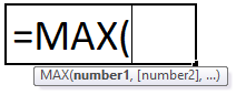
MAX(number1, [number2], …)
The MAX function syntax has the following arguments:
-
Number1, number2, … Number1 is required, subsequent numbers are optional. 1 to 255 numbers for which you want to find the maximum value.
Remarks
-
Arguments can either be numbers or names, arrays, or references that contain numbers.
-
Logical values and text representations of numbers that you type directly into the list of arguments are counted.
-
If an argument is an array or reference, only numbers in that array or reference are used. Empty cells, logical values, or text in the array or reference are ignored.
-
If the arguments contain no numbers, MAX returns 0 (zero).
-
Arguments that are error values or text that cannot be translated into numbers cause errors.
-
If you want to include logical values and text representations of numbers in a reference as part of the calculation, use the MAXA function.
Example
Copy the example data in the following table, and paste it in cell A1 of a new Excel worksheet. For formulas to show results, select them, press F2, and then press Enter. If you need to, you can adjust the column widths to see all the data.
|
Data |
||
|
10 |
||
|
7 |
||
|
9 |
||
|
27 |
||
|
2 |
||
|
Formula |
Description |
Result |
|
=MAX(A2:A6) |
Largest value in the range A2:A6. |
27 |
|
=MAX(A2:A6, 30) |
Largest value in the range A2:A6 and the value 30. |
30 |
Need more help?
Return value
The largest value in supplied data
Usage notes
The MAX function returns the largest numeric value in the data provided. The MAX function can be used to return the largest value from any type of numeric data. For example, MAX can return the slowest time in a race, the latest date, the largest percentage, the highest temperature, or the top sales number.
The MAX function takes multiple arguments in the form number1, number2, number3, etc. up to 255 total. Arguments can be a hardcoded constant, a cell reference, or a range, in any combination. MAX ignores empty cells, text values, and the logical values TRUE and FALSE.
Basic Example
The MAX function returns the largest numeric value in supplied data:
=MAX(12,17,25,11,23) // returns 25
When given a range, MAX returns the smallest value in the range:
=MAX(A1:A10) // maximum value in A1:A10Mixed arguments
The MAX function can accept a mix of arguments:
=MAX(5,10)
=MAX(A1,A2,A3)
=MAX(A1:A10,100)
=MAX(A1:A10,C1:C10)
Logical values
The MAX function will ignore logical values and numbers entered as text that appear on the worksheet. However, if such values are provided directly as arguments, MAX will use them:
=MAX(-1,TRUE) // returns 1
=MAX(-1,TRUE,"3") // returns 3
Errors
When MAX encounters an error in a range, it will return an error. To calculate a maximum value while ignoring errors, you can use the AGGREGATE function, which can be configured to ignore errors. See a detailed example here.
Other functions
Excel provides other functions that deal with maximum values and rank:
- To calculate the maximum value with criteria, use the MAXIFS function.
- To retrieve the nth largest value in a data set, use the LARGE function.
- To determine the rank of a number in a set of data, use the RANK function.
Notes
- Arguments can be provided as numbers, names, arrays, or references.
- MAX accepts up to 255 arguments. If arguments contain no numbers, MAX returns 0.
- MAX ignores empty cells, text values, and TRUE and FALSE in references.
- MAX will evaluate numbers as text and logical values supplied directly as arguments.
- To include logical values in a reference, see the MAXA function.
Excel MAX function is categorized under statistical functions in Microsoft Excel. The Excel MAX Formula is used to find out the maximum value from a given set of data/ array. MAX function in Excel returns the highest value from a given set of numeric values.
Excel MAX formula will count numbers but ignore empty cells, text, the logical values TRUE and FALSE, and text values.
Excel MAX formulaThe MAX Formula in Excel is used to calculate the maximum value from a set of data/array. It counts numbers but ignores empty cells, text, the logical values TRUE and FALSE, and text values.read more can be used to calculate the highest salary of the employee, the fastest time/score, the highest expense or revenue amount, etc.
Table of contents
- MAX in Excel
- MAX Formula in Excel
- How to Use MAX Function in Excel?
- MAX in Excel Example #1
- MAX in Excel Example #2
- MAX in Excel Example #3
- MAX in Excel Example #4
- MAX in Excel Example #5
- MAX Function in Excel VBA
- Things to Remember About MAX Function in Excel
- MAX Excel Function Video
- Recommended Articles
MAX Formula in Excel
Below is the formula for MAX in Excel.
MAX formula in excel has at least one compulsory parameter, i.e., number1, and the rest of subsequent numbers are optional.
Compulsory Parameter:
- number1: it is the required number.
Optional Parameter:
- [number2]: Rest subsequent numbers are optional.
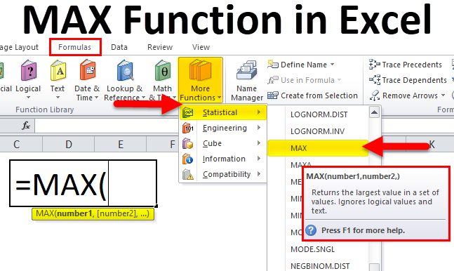
How to Use MAX Function in Excel?
MAX function in excel is very simple and easy to use. Let us understand the working of the MAX Function by some examples. MAX formula in Excel can be used as a worksheet function and as a VBA functionVBA functions serve the primary purpose to carry out specific calculations and to return a value. Therefore, in VBA, we use syntax to specify the parameters and data type while defining the function. Such functions are called user-defined functions.read more.
You can download this MAX Function Excel Template here – MAX Function Excel Template
MAX in Excel Example #1
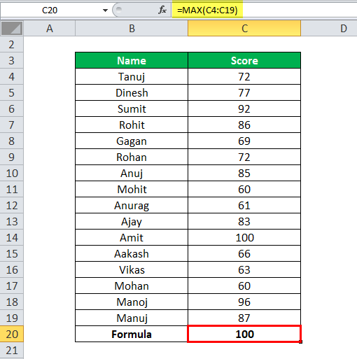
In this example, we have a student database with their score details. Now we need to find out the max score from these students.
Here apply the MAX formula in Excel =MAX(C4:C19)

it will return you the max score from the given list of scores, as shown in the below table.
MAX in Excel Example #2
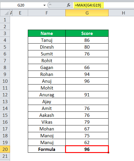
In this example, we have student details with their score, but here some students did not have any score.
Now apply the MAX formula in Excel here =MAX(G4:G19)
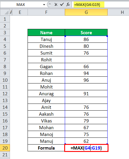
MAX Function ignores the empty cells and then calculates the MAX score from the given data, as shown in the below table.
MAX in Excel Example #3
Suppose we have student details with their score, but some of the student’s score values are Boolean.
apply the MAX formula in Excel here =MAX(J4:J19)
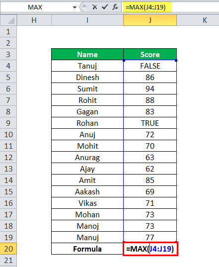
MAX function in Excel ignores these Boolean values cells and then calculates the MAX score from the given data, as shown in the below table.

MAX in Excel Example #4
Suppose we have a list of names, and we have to calculate the name with maximum length.
Here we have to apply the LEN function to calculate the length of the name.
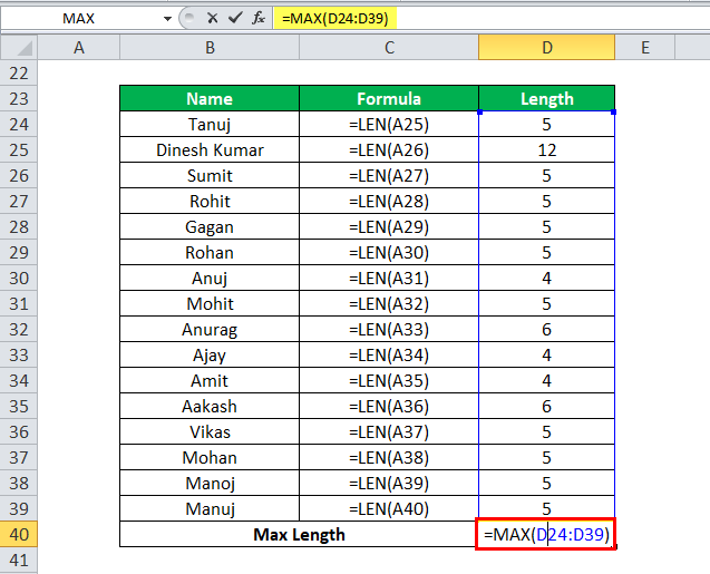
Apply the MAX formula in Excel to find out the name with maximum length.

MAX in Excel Example #5
MAX formula can be used to find the max date from the given set of dates and maximum time from the given time and can be used to find the maximum currency from the given data, as shown in the below table.

MAX Function in Excel VBA
MAX Function in Excel can be used as a VBA function.
Sub Maxcal()
Dim Ans As Integer //declare the Ans as integer
Ans = Applicaltion.WorksheetFunction.Max(Range(“A1:B5”)) // Apply max function on range A1 to B5
MsgBox Ans //Display the max value in the Message box.
End Sub
Things to Remember About MAX Function in Excel
- MAX function through #VALUE! Error if any of the supplied values are non-numeric.
- MAX function on Excel will count numbers but ignore empty cells, text, the logical values TRUE and FALSE, and text values.
- If the MAX function does not have any arguments, then it will return the 0 as output.
MAX Excel Function Video
Recommended Articles
This has been a guide to MAX in Excel. Here we discuss the MAX Formula in excel and how to use the MAX Excel function along with excel example and downloadable excel templates. You may also look at these useful functions in excel –
- MEDIAN Formula in ExcelMEDIAN function in Excel gives the median of a given set of numbers. MEDIAN Identifies the location of the center of a group of numbers in a statistical distribution.read more
- COUNTIF Formula in ExcelThe COUNTIF function in Excel counts the number of cells within a range based on pre-defined criteria. It is used to count cells that include dates, numbers, or text. For example, COUNTIF(A1:A10,”Trump”) will count the number of cells within the range A1:A10 that contain the text “Trump”
read more - Median FormulaThe median formula in statistics is used to determine the middle number in a data set that is arranged in ascending order. Median ={(n+1)/2}thread more
- Max IF Formula in ExcelThe MAX IF formula uses two excel functions (MAX and IF Function) to find the maximum value from all of the logical test’s outcomes. MAX IF is an array formula that allows you to run a logical test multiple times in a data set.read more
- VLOOKUP on Different SheetsVLOOKUP facilitates the users to fetch data from different worksheets by selecting the table array from the respective worksheet of the result looking column. The lookup value must be to the left of the required result column.read more
Excel MAX Function (Table of Contents)
- MAX in Excel
- MAX Formula in Excel
- How to Use MAX Function in Excel?
MAX in Excel
Max function in excel is the simplest form of a mathematical function, which just returns the maximum values out of the selected values or array. We can selected values one by one, or in one go, we can select a complete range of numbers if available in a sequence. It also neglects the blank cells, logical values, and text if any of these comes in a selected range.
MAX Formula in Excel:
Below is the MAX Formula in Excel:
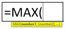
The MAX Formula in Excel has the parameter as below :
- number1, [number2]: The number or cell reference or range arguments can be one or more numeric values from which you want to find the maximum value in Excel.
number1 is a compulsory parameter or argument, whereas the remaining subsequent numbers are an optional argument. From excel 2007 & later versions, it can take up to 255 arguments. The Formula for the ‘MAX’ function is exactly similar or the same as that for the ‘MIN’ function. We can mix literal values along with cell references to find out the maximum value.
e.g. =MAX(D8:D19,100) here literal value in the function is 100.
How to Use MAX Function in Excel?
MAX Function in Excel is very simple and easy to use. Let us understand the working of MAX Function in Excel by some MAX Formula in Excel examples.
You can download this MAX Function Excel Template here – MAX Function Excel Template
MAX Function can be used as a worksheet function and as a VBA function.
Example #1
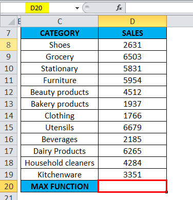
The below-mentioned table contains a category of items in column C (C8 to C19) & sale value in column D (D8 to D19). I need to find out which category has maximum sales in the supermarket. MAX Function in Excel is used on the range of values representing sales by category to extract the highest value.
Let’s apply Max Function in cell “D20”. Select the cell “D20”, where Max Function needs to be applied.
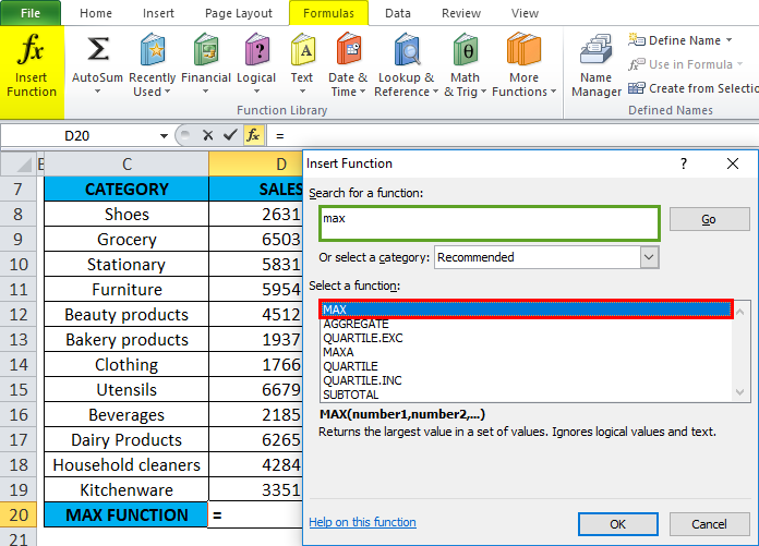
Click the insert function button (fx) under the formula toolbar; a dialog box will appear, type the keyword “MAX” in the search for a function box; MAX Function will appear in select a function box Double click on MAX Function.
A dialog box appears where arguments for MAX Function needs to be filled or entered i.e. =MAX(number1, [number2], … )
=MAX(D8: D19) Here, the sales data is present in the range (D8: D19). To enter the Number 1 argument, click inside cell D8 and you’ll see the cell selected, then Select the cells till D19. So that column range will get selected, i.e. D8: D19. Click ok after entering the number1 argument.
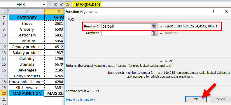
=MAX(D8: D19), i.e. returns the maximum sales value 6679 as a result.
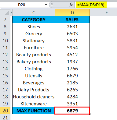
MAX Function has returned the maximum available sales value within a defined range, i.e. 6679 under the utensil’s category.
Example #2
To calculate the maximum or highest score in academics for a specific subject (Mathematics).
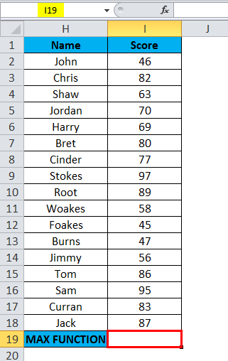
The below-mentioned table below contains the student’s Name in column H (H2 to H18) & each student’Fs score (I2 to I18). I need to find out which student has scored a maximum or highest score in mathematics subject. Here, MAX Function in Excel is used on the range of values representing the score to extract the highest value.
Let’s apply Max Function in cell “I19”. Select the cell “I19”, where Max Function needs to be applied.
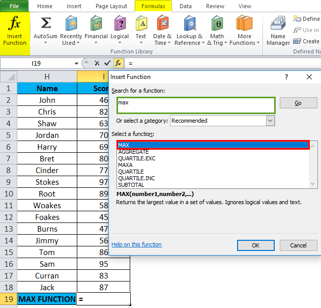
Click the insert function button (fx) under the formula toolbar; a dialog box will appear, type the keyword “MAX” in the search for a function box; MAX Function will appear in select a function box. Double click on MAX Function.
A dialog box appears where arguments for MAX Function needs to be filled or entered i.e. =MAX(number1, [number2], … )
=MAX(I2: I18) Here, the score data is present in the range (I2: I18). To enter the Number 1 argument, click inside cell I2 and you’ll see the cell selected, then Select the cells till I18. So that column range will get selected, i.e.I2: I18. Click ok after entering the number1 argument.
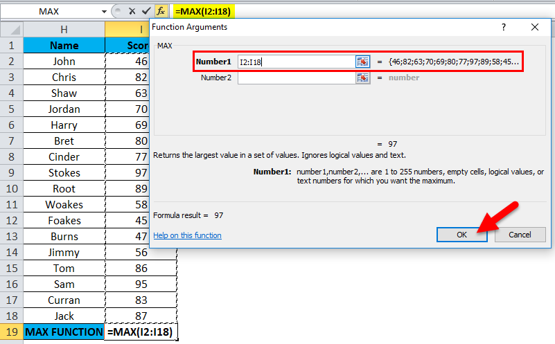
=MAX(I2: I18), i.e. returns the maximum score value 97 as a result.
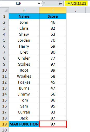
Here, MAX Function has returned the maximum score value within the defined range, i.e. 97, under the score category.
Example #3
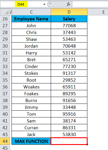
To calculate the maximum or highest Salary for an employee in the company.
The below-mentioned table below contains the Name of the employee in column C (C27 to C43) & the Salary of an employee (D27 to D43). I need to find out which employee is getting the highest or maximum salary in the company. Here, MAX Function in Excel is used on the range of values representing an employee’s salary to extract the highest or maximum value.
Let’s apply Max Function in cell “D44”. Select the cell “D44”, where Max Function needs to be applied.
Click the insert function button (fx) under the formula toolbar; a dialog box will appear, type the keyword “MAX” in the search for a function box; MAX Function will appear in select a function box. Double click on MAX Function.
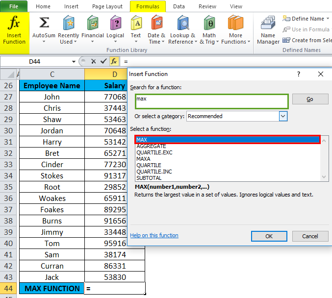
A dialog box appears where arguments for MAX Function needs to be filled or entered i.e. =MAX(number1, [number2], … )
=MAX(D27: D43) Here, the salary data is present in the range (D27: D43). To enter the Number 1 argument, click inside cell D27 and you’ll see the cell selected, then Select the cells till D43. So that column range will get selected, i.e. D27: D43. Click ok after entering the number1 argument.
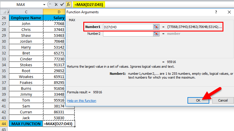
=MAX(D27: D43), i.e. returns the maximum salary of the employee, i.e. 95,916 as a result.
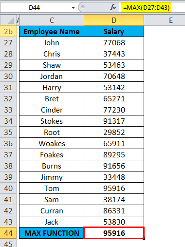
Here, MAX Function has returned the maximum or highest salary of an employee within a defined range, i.e. 95,916.
Things to Remember
- Argument type can be a cell reference, range reference, column reference row reference, numbers, multiple columns/rows & cell, and range names.
- Max Function in Excel ignores numbers entered as text values, empty cells & the logical values TRUE and FALSE & it should not have any error value (#N/A, VALUE, DIV).
- If there are no numbers in a specified range or arguments, it will return 0.
- If there is an error value in the argument or text, it will return #N/A.
- MAX Function in Excel is the same as LARGE function; both return the biggest number.
- #VALUE! error: It Occurs if any non-numeric values are supplied directly to the Max Function.
Recommended Articles
This has been a guide to MAX in Excel. Here we discuss the MAX Formula in Excel and how to use MAX Function in Excel along with practical examples and downloadable excel templates. You can also go through our other suggested articles –
- Excel MAX IF Function
- Excel SUM MAX MIN AVERAGE
- VBA Max
- Excel MIN Function
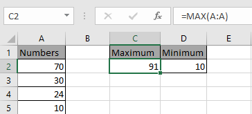
In this article, we will learn How to use the MAX function in Excel.
MAXIMUM or largest value in array
IN Excel, many times we need the lowest or the highest value present in the list. For example finding the largest or maximum sales value in employees dataset. Or finding the largest discount percentage in the products table. Let’s understand the function syntax and an example to illustrate the function usage.
MAX Function in Excel
MAX function returns the maximum number is the range.
Syntax:
array : list of numbers given as array reference in the function. Like values in A1 to A75 be referred as A1:A75
Example :
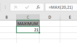
All of these might be confusing to understand. Let’s understand how to use the function using an example. Maximum of two input numbers is done via Formula shown below.
Use the formula
Now we wish to find the Maximum from the entire column.
Here we have 76 numbers in column A.
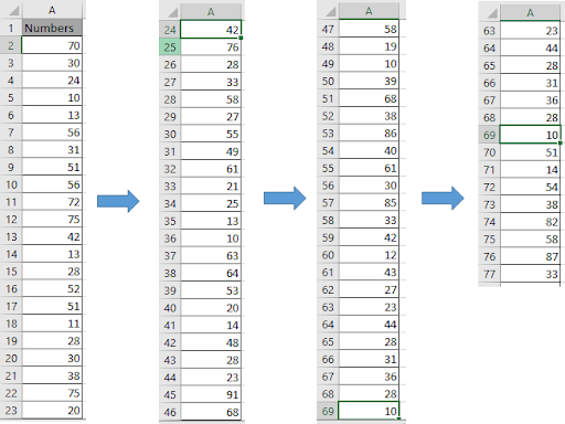
Here we need to Maximum value present in this column. There would two methods
Use the formula
OR
=MAX(A:A)

As you can see you can get the maximum value from the range of numbers. You can get the minimum value from the range using the MIN function in Excel.
MAXA function in Excel
MAXA function is a mathematical function which returns the numerical largest value from an array of numbers given in as input. The MAXA function considers logic values also whereas MAX function doesn’t. MAXA function given a list of values as arguments returns the maximum numeric value in the cell.
MAXA function Syntax:
=MAXA(number1,number2,..)
number : number or array given as cell reference
MAXA function Example:
All of these might be confusing to understand. So, let’s test this formula via running it on the example shown below. Here we have some numbers to test the MAXA function in Excel.
Use the formula:
Here the array of values is given as cell reference. You can also input values as numbers.
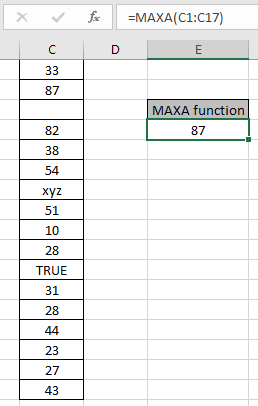
Here the function ignores blank cells, TRUE logic value is considered as 1 & xyz text as zero. The function returns 87 as numerically the largest value from the array C1:C17.
Now consider one more example of MAXA function:
Here we take negative numbers and Logic value in array and take the respective from both MAXA and MAX function
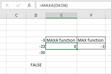
-3 is the numerically the largest value so the MAX function ignores logic values and returns -3 but MAXA considers TRUE as 1 and FALSE as 0 numeric value and returns 0 as result.
Here are some observational notes using the MAX function in Excel shown below.
Notes:
- The formula only works with numbers and text.
- The MAXA function considers logic values TRUE as 1 and FALSE as 0 whereas MAX function ignores.
- The function takes 0 if no number is given in as input.
Hope this article about How to use the MAX function in Excel is explanatory. Find more articles on calculating values and related Excel formulas here. If you liked our blogs, share it with your friends on Facebook. And also you can follow us on Twitter and Facebook. We would love to hear from you, do let us know how we can improve, complement or innovate our work and make it better for you. Write to us at info@exceltip.com.
Related Articles :
How to use the MAX function in Excel | returns the numerical largest value from the given array using the MAX function in Excel
How to use the MIN function in Excel | returns the numerical smallest value from the given array using the MIN function in Excel
How to use the LARGE function in Excel | returns the numerical largest nth value from the given array using the LARGE function in Excel
How to use the ISEVEN function in Excel | returns the TRUE logic value if the number is MAX using the ISEVEN function in Excel.
How to use the ISODD function in Excel | returns the TRUE logic value if the number is ODD using the ISODD function in Excel.
Calculate max if condition match : Get the MAX value from the array having criteria.
How to Use Excel AGGREGATE Function : Use the AGGREGATE function to perform multiple operation with multiple criterias in excel.
COUNTIFS With OR For Multiple Criteria : Count cells having multiple criteria match using the OR function.
How to use wildcards in excel : Count cells matching phrases using the wildcards in excel
Popular Articles :
How to use the IF Function in Excel : The IF statement in Excel checks the condition and returns a specific value if the condition is TRUE or returns another specific value if FALSE.
How to use the VLOOKUP Function in Excel : This is one of the most used and popular functions of excel that is used to lookup value from different ranges and sheets.
How to use the SUMIF Function in Excel : This is another dashboard essential function. This helps you sum up values on specific conditions.
How to use the COUNTIF Function in Excel : Count values with conditions using this amazing function. You don’t need to filter your data to count specific values. Countif function is essential to prepare your dashboard.
Returns the largest value in a given list of arguments
What is the MAX Function?
The MAX Function[1] is categorized under Excel Statistical functions. MAX will return the largest value in a given list of arguments. From a given set of numeric values, it will return the highest value. Unlike MAXA function, the MAX function will count numbers but ignore empty cells, text, the logical values TRUE and FALSE, and text values.
In financial analysis, MAX can be useful in calculating the highest score, the fastest time, the highest expense or revenue amount, etc.
Formula
=MAX(number1, [number2], …)
Number1 and number2 are the arguments used for the function, where Number1 is required and the subsequent values are optional.
In MS Excel 2007 and later versions, we can provide up to 255 number arguments to the MAX function. However, in Excel 2003 and earlier versions, it can only accept up to 30 number arguments.
Arguments can be provided as constants, or as cell references or ranges. If an argument is supplied to the function as a reference to a cell, or an array of cells, the MAX function will ignore blank cells, and text or logical values contained within the supplied cell range. However, logical values and text representations of numbers that are supplied directly to the function will be included in the calculation.
How to use the MAX Function in Excel?
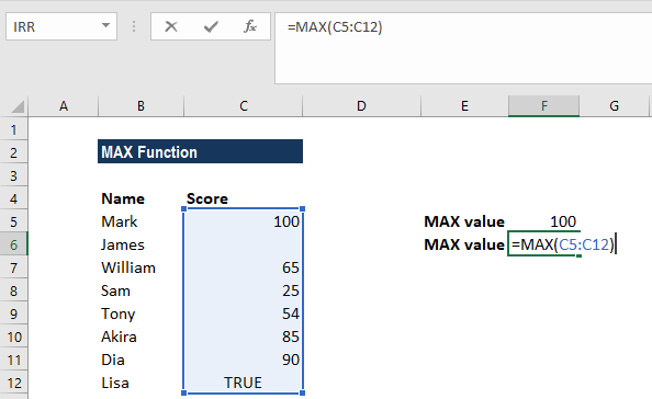
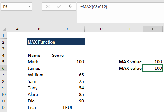
As a worksheet function, the MAX function can be entered as part of a formula in a cell of a worksheet. To understand the uses of the function, let us consider an example:
Example
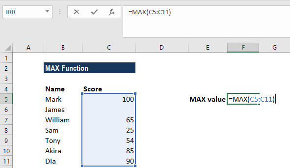
Let us calculate the highest marks from the following data:
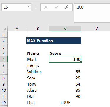
The formula used was:
The MAX function ignored the empty value and returned 100 as the result.
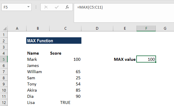
As seen above, MAX will ignore empty values. In this example, if we provide a logical value, the function will ignore it and give the same result, as shown below:
A few things to remember about the MAX Function
- #VALUE! error – Occurs if any values that are provided directly to the MAX function are non-numeric.
- If the arguments contain no numbers, MAX returns 0.
- The primary difference between MAX and MAXA is that MAXA evaluates TRUE and FALSE values as 1 and 0, respectively. Hence, if we wish to include logical values, then we need to use the MAXA function.
Click here to download the sample Excel file
Additional Resources
Thanks for reading CFI’s guide to important Excel functions! By taking the time to learn and master these functions, you’ll significantly speed up your financial modeling. To learn more, check out these additional CFI resources:
- Excel Functions for Finance
- Advanced Excel Formulas Course
- Advanced Excel Formulas You Must Know
- Excel Shortcuts for PC and Mac
- See all Excel resources
Article Sources
- MAX Function

This Excel tutorial explains how to use the Excel MAX function with syntax and examples.
Description
The Microsoft Excel MAX function returns the largest value from the numbers provided.
The MAX function is a built-in function in Excel that is categorized as a Statistical Function. It can be used as a worksheet function (WS) in Excel. As a worksheet function, the MAX function can be entered as part of a formula in a cell of a worksheet.
Syntax
The syntax for the MAX function in Microsoft Excel is:
MAX( number1, [number2, ... number_n] )
Parameters or Arguments
- number1
- It can be a number, named range, array, or reference to a number.
- number2, … number_n
- Optional. These are numeric values that can be numbers, named ranges, arrays, or references to numbers. There can be up to 30 values entered.
Returns
The MAX function returns a numeric value.
Applies To
- Excel for Office 365, Excel 2019, Excel 2016, Excel 2013, Excel 2011 for Mac, Excel 2010, Excel 2007, Excel 2003, Excel XP, Excel 2000
Type of Function
- Worksheet function (WS)
Example (as Worksheet Function)
Let’s look at some Excel MAX function examples and explore how to use the MAX function as a worksheet function in Microsoft Excel:
Based on the Excel spreadsheet above, the following MAX examples would return:
=MAX(A2, A3)
Result: 10.5

=MAX(A3, A5, 45)
Result: 45

=MAX(A2:A6)
Result: 200

=MAX(A2:A6, 325)
Result: 325
Frequently Asked Questions
Question: In Microsoft Excel, I want to calculate the largest yearly difference in total between any adjacent year for each company. Below is my spreadsheet with a small sample of 4 years of data.
Right now, I’m using the following formula to calculate the yearly difference:
=IF(AND((MAX(B2:C2)-MIN(B2:C2))>(MAX(C2:D2)-MIN(C2:D2)), (MAX(B2:C2)-MIN(B2:C2))>(MAX(D2:E2)-MIN(D2:E2))), MAX(B2:C2)-MIN(B2:C2), IF((MAX(C2:D2)-MIN(C2:D2))>(MAX(D2:E2)-MIN(D2:E2)), MAX(C2:D2)-MIN(C2:D2), MAX(D2:E2)-MIN(D2:E2)))
I am wondering if there is a way to streamline this and not have such a long and complicated formula.
Answer: Yes, it should be possible to simplify your formula and achieve the same results. By using the ABS function, you could remove some of your IF conditions since you are really looking for the yearly differences as «absolute values». Try replacing your formula with the following:
=MAX(ABS(B2-C2),ABS(C2-D2),ABS(D2-E2))
As you can see in the spreadsheet below, this formula is much simpler and returns the same results.
Question:I’m having a problem finding a specific formula in Excel.
Is there a formula that will tell me the Cell with the highest number rather than tell me the highest number? I.E. if K2 has 15 and is the highest, how do I make a formula that says K2 instead of 15?
Answer: You can use the CELL, INDEX, and MATCH functions in combination with the MAX function to return the cell with the highest value.
For example, if you wanted to find the cell with the highest value in the range K1 to K10, you could use the following formula:
=CELL("address",INDEX(K1:K10,MATCH(MAX(K1:K10),K1:K10,0)))
This would return the result as an absolute reference such as $K$2, as you stated in your example where the cell K2 contained 15 which was the highest value.
MAX function is used to find the largest number in the range passed in as arguments and returns the corresponding value.
MAXA function is used to find the highest value in the specified range and returns the number found.
The main difference between the two functions is that MAX ignores the logical values passed as arguments, and MAXA takes them into account in the search process.
Examples of using functions of MAX and MAXA in Excel
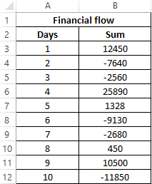
Example 1. An enterprise economist records income and expenses in a single column of an Excel spreadsheet, with income being positive numbers and expenses being negative. Find the maximum expense for the last few days.
Initial data:
For calculation, we use the array formula:
Argument Description:
- B3:B12<0 — condition for checking whether a number belongs to a range of negative numbers;
- ABS(B3:B12) is the return value of the IF function for the found negative numbers.
- (-1) — the multiplier required to return a negative number.
Note: the largest number in the range of negative numbers is, the value of which is closer to zero. In this problem, we were interested in the maximum flow rate, so for the search for the maximum value, the ABS function was used, which returns the modulus of the number.
Result of calculations:
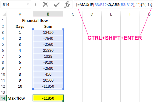
As a result of calculations by the formula, we obtained the maximum amount of expenses using the MAX function, despite the fact that this is a negative number with a minus sign.
Calculation of the maximum and minimum costs in the Excel spreadsheet
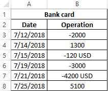
Example 2. The owner of a card connected to Internet banking, has entered into the Excel spreadsheet information about cash receipts on the card, as well as costs. By mistake, some of the cells in the column containing the amount of money got text data. Determine the minimum and maximum transaction costs of funds.
Source data table:
The formula for calculating the minimum cost (array formula):
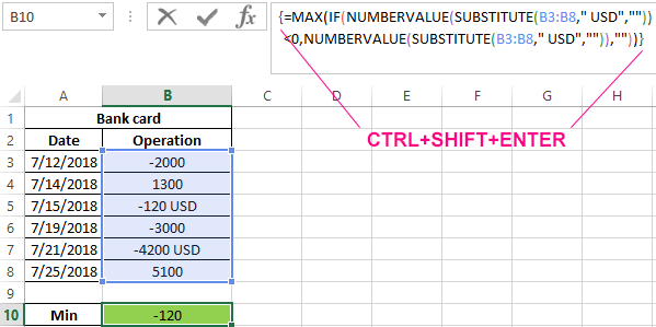
Argument Description:
- NUMBERVALUE(SUBSTITUTE(B3:B8,»USD»,»»)) <0 is an expression that checks the belonging of numbers to a range of negative values. The FAST function replaces part of the string “USD” with an empty value “”, the CHARGE function converts the text data type to a numeric one.
- NUMBERVALUE(SUBSTITUTE(B3:B8,»USD»,»»)) — the range of negative numbers, that is, records only of the costs on the card.
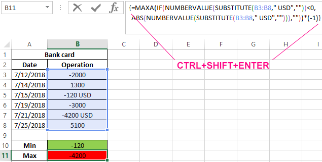
To obtain the highest value of costs, we slightly modify this formula:
The maximum flow rate corresponds to the largest modulus of a negative number (the ABS function is used for this purpose). To return a negative number, the result is multiplied by -1.
The resulting values are:
Finding the maximum value among different data types in Excel
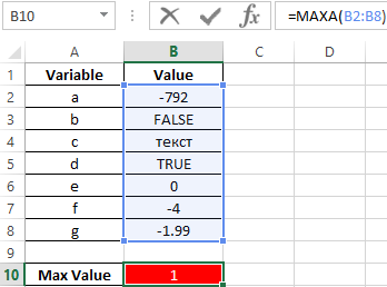
Example 3. A programmer entered the values of variables of different data types into an Excel spreadsheet. Determine the highest value given the data of the logical type.
Source table:
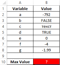
In this case, it is advisable to use the MAXA formula, since some variables contain data of a logical type. The formula for calculating:
The result:
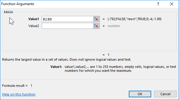
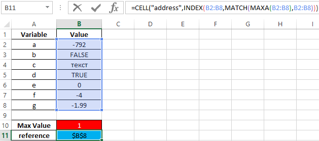
Pay attention to some features of the functions. For example, if in the framework of this example it was required to return a reference to a cell containing the maximum value, you could use the formula:
However, the return value is not true:
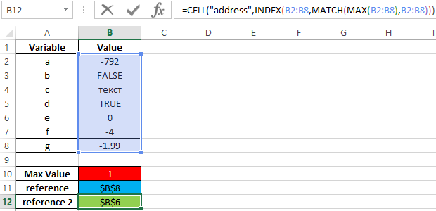
But in the case of using the function MAX, ignoring logical values, the result will be correct:
Result:
Features of using functions of MAX and MAXA in Excel
The MAX function has the following syntax notation:
=MAX(number1,[number2],…)
Argument Description:
- number1 is a required argument characterizing the first value of the range of numeric data (array, vector), among which you need to find the maximum value.
- [number2] … — the second and subsequent optional arguments characterizing the second and subsequent numerical values of the studied range.
The MAXA function has the following syntax notation:
=MAXA(value1,[value2],…)
Argument Description:
- value1 is an obligatory argument characterizing the first occurrence of the range of the studied data.
- [value2] … — the second and subsequent optional arguments characterizing the second and subsequent occurrences.
Notes:
- Both considered functions accept as arguments names, data of numerical, logical, reference and text data types.
- The MAX function takes into account logical values only if they are explicitly passed as an argument (for example, (TRUE; -5; FALSE) returns the value 1, but the arguments (A1; A2; A3) return the value -5 if A1 = TRUE , A2 = -5, A3 = FALSE). The MAXA function in calculations takes into account even references to cells containing data of a logical type.
- When using functions for Date data, the maximum value will be returned in the Excel time code.
- If the array or data range passed as arguments contains only text data, the result of the MAX and MAXA functions is 0. If the array or the data range also contains text values and empty cells, the MAX and MAXA functions ignore in the calculations.
- The MAXA function is convenient for use in cases where it is necessary to transmit a reference to a data range containing textual representations of numbers and logical values that must be taken into account in the calculations. Otherwise, use the MAX function.
- Since the functions in question have no analogs with a logical check (for example, the SUM function has an analog with the SUMIF test), to check the conditions, use the following record =MAX(IF(checked_expression,array1,array2)), where array1 and array2 are options for the function arguments MAX depending on the result of executing the checked expression).
Download examples MAX and MAXA functions in Excel
The MAX and MAXA functions can be used as array formulas, which is convenient when used together with logical functions.