
Excel for Microsoft 365 Excel for Microsoft 365 for Mac Excel for the web Excel 2021 Excel 2021 for Mac Excel 2019 Excel 2019 for Mac Excel 2016 Excel 2016 for Mac Excel 2013 Excel 2010 Excel 2007 Excel for Mac 2011 Excel Starter 2010 More…Less
This article describes the formula syntax and usage of the ERF function in Microsoft Excel.
Description
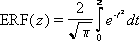
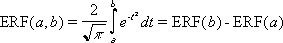
Returns the error function integrated between lower_limit and upper_limit.
Syntax
ERF(lower_limit,[upper_limit])
The ERF function syntax has the following arguments:
-
Lower_limit Required. The lower bound for integrating ERF.
-
Upper_limit Optional. The upper bound for integrating ERF. If omitted, ERF integrates between zero and lower_limit.
Remarks
-
If lower_limit is nonnumeric, ERF returns the #VALUE! error value.
-
If upper_limit is nonnumeric, ERF returns the #VALUE! error value.
Example
Copy the example data in the following table, and paste it in cell A1 of a new Excel worksheet. For formulas to show results, select them, press F2, and then press Enter. If you need to, you can adjust the column widths to see all the data.
|
Formula |
Description |
Result |
|---|---|---|
|
=ERF(0.745) |
Error function integrated between 0 and 0.74500 |
0.70792892 |
|
=ERF(1) |
Error function integrated between 0 and 1. |
0.84270079 |
Need more help?
Want more options?
Explore subscription benefits, browse training courses, learn how to secure your device, and more.
Communities help you ask and answer questions, give feedback, and hear from experts with rich knowledge.
Содержание
- Метод WorksheetFunction.Erf (Excel)
- Синтаксис
- Параметры
- Возвращаемое значение
- Замечания
- Поддержка и обратная связь
- IFERROR function
- Syntax
- Remarks
- Examples
- Example 2
- Need more help?
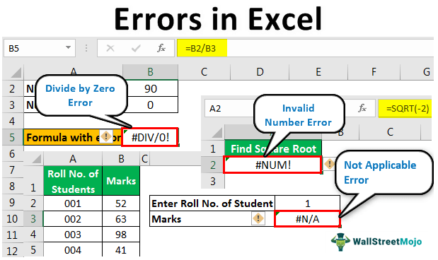
- Errors in Excel
- List of Various Excel Errors
- Types of Errors in Excel with Examples
- 1 – #DIV/0 Error
- 2 – #N/A Error
- 3 – #NAME? Error
- 4 – #NULL! Error
- 5 – #NUM! Error
- 6 – #REF! Error
- 7 – #VALUE! Error
- 8 – ###### Error
- 9 – Circular Reference Error
- Function to Deal with Excel Errors
- 1 – ISERROR Function
- 2 – AGGREGATE Function
- Things to Remember
- Recommended Articles
Метод WorksheetFunction.Erf (Excel)
Возвращает функцию ошибок, интегрированную между lower_limit и upper_limit.
Эта функция была заменена одной или несколькими новыми функциями, которые могут обеспечить повышенную точность и имена которых лучше отражают их использование. Эта функция по-прежнему доступна для совместимости с более ранними версиями Excel. Однако если обратная совместимость не требуется, следует рассмотреть возможность использования новых функций, так как они более точно описывают их функциональность.
Дополнительные сведения о новой функции см. в методе Erf_Precise .
Синтаксис
expression. Erf (Arg1, Arg2)
Выражение Переменная, представляющая объект WorksheetFunction .
Параметры
| Имя | Обязательный или необязательный | Тип данных | Описание |
|---|---|---|---|
| Arg1 | Обязательный | Variant | Lower_limit — нижняя граница для интеграции Erf. |
| Arg2 | Необязательный | Variant | Upper_limit — верхняя граница для интеграции Erf. Если этот параметр опущен, Erf интегрируется от нуля до lower_limit. |
Возвращаемое значение
Double
Замечания
Если lower_limit не является числом, Erf возвращает #VALUE! значение ошибки.
Если lower_limit является отрицательным, Erf возвращает #NUM! значение ошибки.
Если upper_limit не является числом, Erf возвращает #VALUE! значение ошибки.
Если upper_limit является отрицательным, Erf возвращает #NUM! значение ошибки.
Поддержка и обратная связь
Есть вопросы или отзывы, касающиеся Office VBA или этой статьи? Руководство по другим способам получения поддержки и отправки отзывов см. в статье Поддержка Office VBA и обратная связь.
Источник
IFERROR function
You can use the IFERROR function to trap and handle errors in a formula. IFERROR returns a value you specify if a formula evaluates to an error; otherwise, it returns the result of the formula.
Syntax
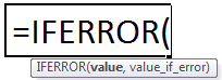
The IFERROR function syntax has the following arguments:
value Required. The argument that is checked for an error.
value_if_error Required. The value to return if the formula evaluates to an error. The following error types are evaluated: #N/A, #VALUE!, #REF!, #DIV/0!, #NUM!, #NAME?, or #NULL!.
If value or value_if_error is an empty cell, IFERROR treats it as an empty string value («»).
If value is an array formula, IFERROR returns an array of results for each cell in the range specified in value. See the second example below.
Examples
Copy the example data in the following table, and paste it in cell A1 of a new Excel worksheet. For formulas to show results, select them, press F2, and then press Enter.
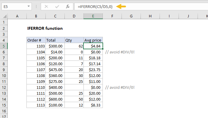
=IFERROR(A2/B2, «Error in calculation»)
Checks for an error in the formula in the first argument (divide 210 by 35), finds no error, and then returns the results of the formula
=IFERROR(A3/B3, «Error in calculation»)
Checks for an error in the formula in the first argument (divide 55 by 0), finds a division by 0 error, and then returns value_if_error
Error in calculation
=IFERROR(A4/B4, «Error in calculation»)
Checks for an error in the formula in the first argument (divide «» by 23), finds no error, and then returns the results of the formula.
Example 2
Error in calculation
Checks for an error in the formula in the first argument in the first element of the array (A2/B2 or divide 210 by 35), finds no error, and then returns the result of the formula
Checks for an error in the formula in the first argument in the second element of the array (A3/B3 or divide 55 by 0), finds a division by 0 error, and then returns value_if_error
Error in calculation
Checks for an error in the formula in the first argument in the third element of the array (A4/B4 or divide «» by 23), finds no error, and then returns the result of the formula
Note: If you have a current version of Microsoft 365, then you can input the formula in the top-left-cell of the output range, then press ENTER to confirm the formula as a dynamic array formula. Otherwise, the formula must be entered as a legacy array formula by first selecting the output range, input the formula in the top-left-cell of the output range, then press CTRL+SHIFT+ENTER to confirm it. Excel inserts curly brackets at the beginning and end of the formula for you. For more information on array formulas, see Guidelines and examples of array formulas.
Need more help?
You can always ask an expert in the Excel Tech Community or get support in the Answers community.
Источник
Errors in Excel


List of Various Excel Errors
MS Excel is popular for only its most useful automatic calculation feature, which we achieve by applying various functions and formulas. But while using formulas in Excel cell, we get multiple types of errors.
Table of contents
The error can be:
- #DIV/0
- #N/A
- #NAME?
- #NULL!
- #NUM!
- #REF!
- #VALUE!
- #####
- Circular Reference
You are free to use this image on your website, templates, etc., Please provide us with an attribution link How to Provide Attribution? Article Link to be Hyperlinked
For eg:
Source: Errors in Excel (wallstreetmojo.com)
We have various functions to deal with these errors, which are –
Types of Errors in Excel with Examples
1 – #DIV/0 Error
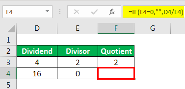
#DIV/0! Error is received when we work with a spreadsheet formula, which divides two values in a formula and the divisor (the number being divided by) is zero. It stands for divide by zero error.
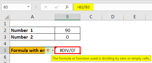
Here, in the above image, we see that number 90 is divided by 0. That is why we get the #DIV/0! Error.
How to Resolve this Error?
The first and foremost solution is to divide only with cells with a value not equal to zero. But there are situations when we also have empty cells in a spreadsheet. In that case, we can use the IF function as below.
Example – IF Function to Avoid #DIV/0 Error
Follow the steps below to use the IF function to avoid the #DIV/0! Error.
- Suppose we are getting a #DIV/0! Error as follows:

To avoid this error, we can use the IF function as follows:
2 – #N/A Error
This error means “no value available” or “not available.” It indicates that the formula cannot find the value that we suppose it may return.
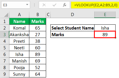
- When the source data and the lookup value are not of the same data type:
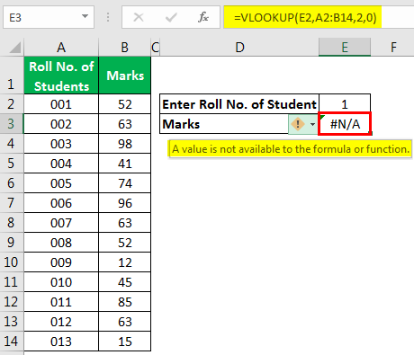
In the above example, we have entered “Roll No. of Students” as a number, but the roll numbers of students are stored as text in the source data. That is why the #N/A error appears.
Solution 1: To enter the Roll number as text

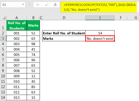
Solution 2: Use the TEXT Function
We can use the TEXT function in the VLOOKUP function for the lookup_value argument to convert entered numbers to TEXT.

We could also use the IFERROR function in excel to display the message if VLOOKUP cannot find the referenced value in the source data.
3 – #NAME? Error
This error is displayed when we usually misspell the function name.
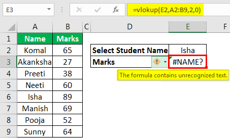
We can see in the above image that VLOOKUP is not spelled correctly; that is why #NAME? Error is being displayed.
To resolve the error, we need to correct the spelling.
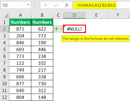
4 – #NULL! Error
We get this error when we do not use the space character appropriately. The space character is called the “intersect operator,” which specifies the range that intersects each other at any cell.
In the below image, we have used the space character, but the ranges A2:A12 and B2:B12 are not intersecting; that is why this error is displayed.
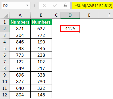
In the below image, we can see that the sum of range B2:B12 is being displayed in cell D2 as while specifying a range for SUM function, we have picked up two references (with space character), which overlap each other for range B2:B12. That is why the sum of the B2:B12 range is displayed.
#NULL! an error can also be displayed when we use intersect operator (space character) instead of:
- Mathematical Operator (Plus Sign) to sum.
- Range Operator (Colon Sign) to specify the start and end cell for a range.
- Union Operator (Comma Sign) to separate individual cell references.
5 – #NUM! Error
This error is usually displayed when a number for any function argument is found invalid.
Example 1

To solve the error, we need to make the number positive.

Example 2
MS Excel has a range of numbers that we can use. The number smaller than the shortest number or number greater than the longest number due to the function can return an error.

Here, we can see that we have written the formula as 2^8000, which yields results greater than the longest number; that is why #NUM! Error is being displayed.
6 – #REF! Error
This error stands for reference error. This error usually comes when
- We accidentally deleted the cell which we referenced in the formula.
- We cut and paste the referenced cell in different locations.

As we deleted cell B7, then cell C7 shifted left to take the place of B7, and we got a reference error in the formula as we deleted one of the referenced cells of the formula.
7 – #VALUE! Error
This error comes when we use the wrong data type for a function or formula. For example, we can add only numbers. But if we use any other data type like text, this error will be displayed.

8 – ###### Error
Example
In the below image, dates and times are written in the cells. But, as column width is not enough, ##### is being displayed.

To resolve the error, we need to increase the column width as per requirement using the “Column Width” command available in the “Format” menu in the “Cell Size” group under the “Home” tab, or we can double click on the right border of the column.

9 – Circular Reference Error
This type of error comes when we reference the same cell in which we are writing the function or formula.

The above image shows that we have a sum of 0 as we have referenced B4 in the B4 cell itself for calculation.

To resolve the error, we need to remove the reference for the B4 cell.

Function to Deal with Excel Errors
1 – ISERROR Function
This function is used to check whether there would be an error after applying the function or not.

2 – AGGREGATE Function
This function ignores error values. Therefore, when we know that there can be an error in the source data, we need to use this function instead of the SUM, COUNT function, etc.
Example

Things to Remember
- To resolve any error in the formula, we can take online help also. First, we need to click on the “Insert Function” button under the “Formulas” tab and choose “Help on this function.”

- To avoid the #NAME? Error, we can choose the desired function from the drop-down list opened when we start typing any function in the cell, followed by the “=” sign. Next, we need to press the “Tab” button on the keyboard to select a function.
Recommended Articles
This article is a guide to Errors in Excel. Here, we discuss the top types of errors in Excel and functions to deal with them with the help of examples. You can learn more about Excel from the following articles: –
Источник
If you have errors in Excel functions, this guide will help you.
Recommended
Speed up your PC today with this easy-to-use download.
g.The Excel IFERROR target returns a customizable result when an absolute formula generates an error, and a reliable default result when an error is likely not to be found. IFERROR is an elegant process for finding and handling errors without the more complex nested IF claims. The value you supply for error conditions.
g.
When to use the iferror function in a formula?
Excel to Microsoft 365 Excel fits Microsoft 365 for Mac Excel for the web Excel 2021 Excel 2021 for Mac Excel 2019 Excel 2019 combined with Mac Excel 2016 Excel 2016 for Mac Excel 2013 Excel Web App Excel 2010 Excel 2007 Excel for Mac 2011 Excel Starter 2010 More … Less
Excel for Microsoft 365 Excel for Microsoft 365 for Mac Excel for the web Excel 2021 Excel 2021 for Mac Excel 2019 Excel 2019 linked to Mac Excel 2016 Excel 2016 for Mac Excel 2013 Excel Web App Excel 2010 Excel 2007 Excel for Mac 2011 Excel Starter 2010 More … Less
What are the functions of error?
Use the IFRESCRIPTION function in Excel to return a different result, such as text, in the event of a baby food failure.
1. For example, Excel returns # DIV / 0! Since you were wrong, the formula tries to divide a large number by 0.
2. If the criterion is assessed as an error, theThe IFERROR function below returns a benevolent message.
3. If the formula does not currently generate a significant error, the IFERROR function simply returns the result of the formula.
For example,
4.Excel will return a # N / A error if any of our VLOOKUP functions cannot find a match.
5.If this VLOOKUP fails, IFERROR returns the friendly message below.
6. If the VLOOKUP function does not always generate an error, the IFERROR function simply returns the result in the VLOOKUP function.
Note. The IFERROR runtime detects the following errors: # DIV / 0!, # N / A, #VALUE!, #REF!, #NUM!, #NAME? combined with #NULL !. For example, the described SIERREUR function also captures #NAME? An error if you misspelled the VLOOKUP term. Use IFNA next to Excel 2013 or later to only detect # N / A errors.
This Excel tutorial shows how to use the Excel IFERROR function with syntax and examples.
Description
The Microsoft Excel iferror function returns an alternate value if the formula results in this error. For example, it is used like # N / A, #VALUE!, #REF!, # DIV / 0!, #NUM!, #NAME? or # EMPTY.
IFERROR a is a built-in Excel function that is classified as a meaningful Boolean function. It might be because you were using the Worksheet (WS) function in Excel. As a worksheet function, some iferror function can even be entered as part of a formula, simply by using a worksheet cell.
What does if Iserror mean in Excel?
If you want to follow this tutorial positively, download most of the sample tables.
Syntax
IFERROR (formula; alternative_value)
Parameters Or Arguments
How do you use the error function in Excel?
- Formula
- Formula or exam you want to test.
- alternate_value
- An alternate value that is returned if the formula gives the best error value (# N / A, #VALUE!, #REF!, # DIV / 0!, #NUM!, #NAME?, or #NULL). Otherwise, if no error occurs, Will usually returns the result, including the formula.
Back
IF-ERROR Returns Any Data Type Such As String, Number, Date, Etc.
Applies To
- Excel for Office 365, Excel 2019, Excel 2016, Excel 2013, Excel 2011 for Mac, Excel 12M 2010, Excel 2007
Type With Function
- Spreadsheet Function (WS)
Example (as Worksheet Function)
When to use if error function in Excel?
Let’s take a look at some examples of Excel IFERROR functions and see how the IFERROR function can be used like almost any Microsoft Excel worksheet function on the market:
Based on the above Excel spreadsheet, column D contains the new formula for calculating the unit price (for example, cell D3 contains plan A3 / B3). Since cells B3 and B6 contain 0 values, the formula is returned in the format # DIV / 0! Errors in cells D3 and D6.
NS.
Recommended
Is your PC running slow? Do you have problems starting up Windows? Don’t despair! ASR Pro is the solution for you. This powerful and easy-to-use tool will diagnose and repair your PC, increasing system performance, optimizing memory, and improving security in the process. So don’t wait — download ASR Pro today!

Columns use the IFEROR function to return any other value of 0 if a particular formula results in an error.
For example, the IFEROR function will return a value that includes 0 (that is: the selection value) up to cell E3, because A3 / B3 results in our # DIV / 0! Error:
= IF ERROR (A3 / B3,0)Result: 0
= IF ERR БКА (A4 / B4,0)Price: $ 0.50

Since A4 / B4 does not throw an error, the function will return a formula advance, which is probably $ 0.50.
IFERROR is a mind-blowing feature that can help you find and fix errors in your personal Excel formulas.
Speed up your PC today with this easy-to-use download.
Which is an example of an error in Excel?
When to use the iserror function in Excel?
How do you use the error function in Excel?
Returns a matching number that corresponds to one of the error values in Microsoft Excel, or returns a #N / A human error if there is no error. You can use ERRORS. Enter TYPE in your IF function to check each error value and return the production line for example.
What are the functions of error?
In statistics, the error function for non-negative values with respect to x has the following interpretations: for a random number Y, normally distributed when it comes to the mean value 0 and the standard alternative 1√2, erf x is declared in the opinion of experts Probability Y falls [- x , X].
What are the types of errors in Excel?
Le Funzioni Di Errore Eccellono
Fonctions D Erreur Excel
오류 함수 엑셀
Funkcii Oshibok Excel
Funkcje Bledow Excel
Funcoes De Erro Excel
Fehlerfunktionen Excel
Funciones De Error Excel
Fout Functies Excel
Felfunktioner Excel
What is IFERROR Function in Excel?
The IFERROR function in Excel checks a formula (or a cell) for errors and returns a specified value in place of the error. This returned value can be a text message, an empty string, a logical value, a number, etc. The errors handled by the function include “#N/A,” “#DIV/0!,” “#NAME?,” and so on.
For example, cells A1, A2, and A3 contain the numbers 24, 35, and 78 respectively. We perform the following tasks in the given sequence:
- To find the minimum number among the listed ones, we enter the formula “=MN(A1:A3)” in cell A4. It returns the “#NAME?” error because the correct function is MIN.
- To return a custom message, we enter the formula “=IFERROR(MN(A1:A3),”incorrect function name”)” in cell A4. It returns the text “incorrect function name” (without the double quotation marks).
In this way, the IFERROR excel function replaces the error message (#NAME?) with a customized text string (incorrect function name).
In Excel, errors are displayed on account of multiple reasons. The IFERROR function detects and deals with these errors the way the user wants.
The purpose of using the IFERROR function is to return a customized and specified result in case a formula evaluates to an error. However, if no error is detected, the function returns the output of the formula.
The IFERROR function is categorized under the Logical functions of Excel.
Table of contents
- What is IFERROR Function in Excel?
- Syntax
- How to Use IFERROR Excel?
- #1–“#N/A” Error
- #2–“#DIV/0!” Error
- #3–“#NAME?” Error
- #4–“#NULL!” Error
- #5–“#NUM!” Error
- #6–“#REF!” Error
- #7–“#VALUE!” Error
- Frequently Asked Questions
- Recommended Articles
- How to Use IFERROR Excel?
Syntax
The syntax of the IFERROR excel function is shown in the following image:
The function accepts the following arguments:
- Value: This is the value to be checked for errors. It can be a cell reference, formula, value or expression.
- Value_if_error: This is the output returned in case an error is found. It can be a text string, blank cell, number, logical value, and so on.
Both the preceding arguments are mandatory.
How to Use IFERROR Excel?
Let us go through some examples to understand how the IFERROR function handles the Excel errorsErrors in excel are common and often occur at times of applying formulas. The list of nine most common excel errors are — #DIV/0, #N/A, #NAME?, #NULL!, #NUM!, #REF!, #VALUE!, #####, Circular Reference.read more. Every example covers one Excel error.
You can download this IFERROR Function Excel Template here – IFERROR Function Excel Template
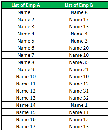
#1–“#N/A” Error
The following table shows the names of some employees segregated in two columns titled “list of emp A” and “list of emp B.” Every name is written as “name” followed by a number. Some names are common to both the columns, while some are present in just one column.
We want to create an excel listA list can be created in Excel to define a list of items/values as predefined values. It may be created using the Data Validation tool so that users may select from a list rather than entering their own values.read more that separates the common names (present in both the columns) from those absent in the first column (list of emp A). Use the following functions:
- The VLOOKUPThe VLOOKUP excel function searches for a particular value and returns a corresponding match based on a unique identifier. A unique identifier is uniquely associated with all the records of the database. For instance, employee ID, student roll number, customer contact number, seller email address, etc., are unique identifiers.
read more function of Excel must look up values in the first column (list of emp A). - The IFERROR function of Excel must return the text string “name not in list A” for all “#N/A” errors.
The steps to apply the VLOOKUP and IFERROR functions (with reference to the current example) are listed as follows:
Step 1: Enter the following VLOOKUP formula in cell C2.
“=VLOOKUP(B2,$A:$A,1,0)”
Press the “Enter” key. Drag the formula downwards till the cell C18. The output of the VLOOKUP formula is shown in column C of the following image.
The VLOOKUP formula looks for a name of column B in column A. It returns the “#N/A” error (in column C) for the names that are absent in column A. Such names could not be found in column A as they are present only in column B.
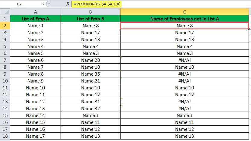
Step 2: Replace the “#N/A” errors (shown in column C of the preceding image) with the text string “name not in list A.” For this, enter the following formula in cell C2.
“=IFERROR(VLOOKUP(B2,$A:$A,1,0),”Name not in list A”)”
Press the “Enter” key. Drag the IFERROR formula till cell C18.
For the ease of understanding, we have displayed the formulas of column C in the succeeding image. Some cells of column C are shown in green. These are the ones that had returned the “#N/A” error in the preceding step (step 1).
The formula “VLOOKUP(B2,$A:$A,1,0)” becomes the first argument and the string “name not in list A” becomes the second argument of the IFERROR function.
The IFERROR function checks the first argument for an error. If the VLOOKUP formula evaluates to an error, the second argument of the IFERROR function is returned. It has already been stated that the VLOOKUP formula evaluates to an error if the lookup value is not found in column A.

Step 3: The output of the IFERROR formula appears in column C, as shown in the succeeding image.
The IFERROR function returns the name if the VLOOKUP formula does not evaluate to an error. However, if the VLOOKUP formula does evaluate to an error, the IFERROR function returns the string “name not in list A.”
In this way, all the “#N/A” errors have been replaced by the text string “name not in list A.” This string implies that the particular name is not in list A (column A).
Hence, “name 20,” “name 35,” “name 21,” “name 31,” and “name 32” are present in column B but not in column A. The names common to both the columns (shown without color) have been separated (in column C) from those absent in column A (shown in green).

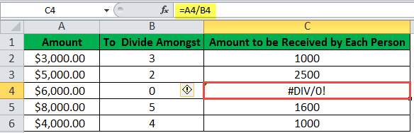
#2–“#DIV/0!” Error
The following table shows some amounts (in $) in the first column titled “amount.” We want to distribute every amount equally among the corresponding number of people mentioned in the second column named “to divide amongst.”
Use the following formulas or functions:
- The division formula must divide the amounts among the stated number of people.
- The IFERROR function must return the text string “no of person < 1” for all “#DIV/0!” errors.
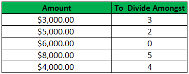
The steps to apply the division formula and the IFERROR function are listed as follows:
Step 1: Enter the following division formula in cell C2.
“=amount/number of people” or “A2/B2”
Press the “Enter” key. Drag the formula downwards till cell C6. The output of the division formula is shown in column C of the following image.
Cell C4 shows the “#DIV/0!” error because the number of people (in cell B4), i.e., the denominator is zero.
Note: In Excel, any number divided by zero returns the “#DIV/0!” error.
Step 2: To replace the “#DIV/0!” error with the text string “no of person < 1,” enter the following formula in cell C2.
“=IFERROR((A2/B2),”No of Person < 1″)”
Press the “Enter” key. Drag the formula till cell C6. The output appears in column C, as shown in the following image.
In cases where the argument “A2/B2” does not evaluate to an error, the IFERROR formula returns the amount (in column C). Wherever the first argument (A2/B2) evaluates to an error, the text string “no of person < 1” is returned. This text string (in cell C4) implies that the number of persons among which $6,000 is to be divided is less than 1.
Hence, the amounts listed in column A have been divided among the number of people stated in column B. The amount received by each person is stated in column C.

#3–“#NAME?” Error
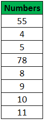
The following list shows some numbers to be added. Use the following functions:
- The SUM function in ExcelThe SUM function in excel adds the numerical values in a range of cells. Being categorized under the Math and Trigonometry function, it is entered by typing “=SUM” followed by the values to be summed. The values supplied to the function can be numbers, cell references or ranges.read more must sum the given numbers.
- The IFERROR function of Excel must return the text string “typed wrong formula” for all “#NAME?” errors.
The steps to apply the SUM and the IFERROR function are listed as follows:
Step 1: Enter the following formula in cell C2.
“=SU(A2:A9)”
The same is shown in the succeeding image.
Press the “Enter” key. The “#NAME?” error appears in cell C2. This is because we have mistakenly entered the function name as “SU” instead of “SUM.”
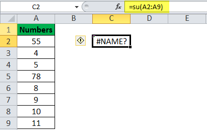
Step 2: To replace the “#NAME?” error with the text string “typed wrong formula,” enter the following formula in cell C2.
“=IFERROR(SU(A2:A9),”Typed Wrong Formula”)”
Press the “Enter” key. The formula is shown in the following image.

Step 3: The output appears in cell C2 of the following image. Hence, the IFERROR function has returned the text string “typed wrong formula” in cell C2. This string implies that the name of the function (SUM) has been typed incorrectly.
The given text string is returned because there is an error in the first argument [SU(A2:A9)] of the IFERROR function. Had we entered the correct function name (SUM), the output of the IFERROR formula (in cell C2) would have been the sum of the listed numbers, i.e., 180.

#4–“#NULL!” Error
The following list shows three numbers in the range A2:A4. We want to sum the numbers using the following formulas or functions:
- The arithmetic operator “plus” (+) must be used to add the numbers in cells A2, A3, and A4.
- The IFERROR function must return the total of the listed numbers.

The steps to use the plus sign (+) and the IFERROR function are listed as follows:
Step 1: Enter the following formula in cell A5.
“=A2+A3 A4”
Press the “Enter” key. The “#NULL!” error appears in cell A5, as shown in the following image. This error appears because we have forgotten to enter the relevant arithmetic operator before the reference A4. Rather, we have mistakenly entered a space before A4.
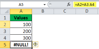
Step 2: To replace the “#NULL!” error with the total of the listed numbers in column A, enter the following formula in cell A5.
“=IFERROR((A2+A3 A4),(SUM(A2:A4)))”
Press the “Enter” key.
The first argument, “A2+A3 A4,” is checked for an error. The second argument, “SUM(A2:A4),” is the “value_if_error.” This implies that if the first argument evaluates to an error, the function returns the output of the second argument “SUM(A2:A4).”
Hence, the IFERROR formula returns the sum 600 in cell A5, as shown in the following image.

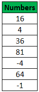
#5–“#NUM!” Error
The following list shows some numbers. We want to find the square roots of these numbers. Use the following functions:
- The SQRT function in Excel must calculate the square roots of the given numbers.
- The IFERROR function must return the text string “a negative number” for all “#NUM!” errors.
The steps to apply the SQRT FunctionThe Square Root function is an arithmetic function built into Excel that is used to determine the square root of a given number. To use this function, type the term =SQRT and hit the tab key, which will bring up the SQRT function. Moreover, this function accepts a single argument.read more and the IFERROR functions are listed as follows:
Step 1: Enter the following SQRT formula in cell B2.
“=SQRT(A2)”
Press the “Enter” key. Drag the formula downwards till cell B8. The output of the SQRT function is shown in column B of the following image.
The SQRT function helps calculate the square root of a number. However, the square root of a negative number does not exist. So, the SQRT function returns “#NUM!” errors for such numbers.
Step 2: To replace the “#NUM!” errors with the text string “a negative number,” enter the following formula in cell B2.
“=IFERROR(SQRT(A2),”A Negative Number”)”
Press the “Enter” key. Drag the formula till cell B8. The output of the formula is shown in column B of the following image.
The IFERROR function returns the result of the SQRT formula for all positive numbers. For the negative numbers, the IFERROR function returns the text “a negative number.” This text string notifies the user that the number whose square root needs to be found is negative.
Hence, the square roots of the listed numbers have been calculated and the resulting “#NUM!” errors have been replaced with a custom message (a negative number).

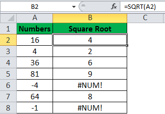
#6–“#REF!” Error
The following image shows two numbers in cells A2 and A3. These numbers have been divided with the help of the formula (=A2/A3) entered in cell C2. We want to delete row 3. Use the following techniques and functions:
- The row 3 must be deleted by right-clicking its header and choosing “delete.”
- The IFERROR function of Excel must return the text string “reference deleted” for the “#REF!” errors.

The steps to delete row 3 and apply the IFERROR function are listed as follows:
Step 1: Select row 3 by clicking the header (3) appearing on the leftmost side of the Excel sheet. Right-click the selection and choose “delete” from the context menu.
The row 3 is deleted and the “#REF!” error appears in cell C2, as shown in the following image.
The cell A3 was a part of the formula entered in cell C2. Since Excel is unable to locate the value (or cell reference) of the denominator, it returns the “#REF!” error in cell C2.
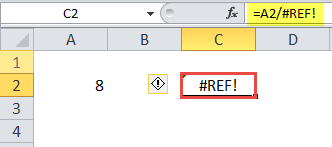
Step 2: To replace the “#REF!” error with the string “reference deleted,” enter the following formula in cell C2.
“=IFERROR((A2/#REF!),”Reference Deleted”)”
Press the “Enter” key. The output of the IFERROR formula appears in cell C2 of the following image.
The IFERROR function checks whether the first argument (A2/#REF!) evaluates to an error or not. Since it does return an error, the function returns the second argument (reference deleted) as the output.
The text string “reference deleted” implies that the cell referenceCell reference in excel is referring the other cells to a cell to use its values or properties. For instance, if we have data in cell A2 and want to use that in cell A1, use =A2 in cell A1, and this will copy the A2 value in A1.read more entered in the division formula has been deleted. This text string is the argument “value_if_error.”
Hence, row 3 has been deleted and the resulting “#REF!” error has been replaced by the string “reference deleted.”
#7–“#VALUE!” Error
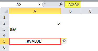
The following image shows two values in cells A2 and A3. We want to add these values. Use the following formulas or functions:
- The arithmetic operator plus (+) must sum up the given values.
- The IFERROR function must return the text string “text can’t add to number” for the “#VALUE!” errors.

The steps to use the plus symbol (+) and the IFERROR function are listed as follows:
Step 1: Enter the following formula in cell A5.
“=A2+A3”
Press the “Enter” key. The “#VALUE!” error appears in cell A5. This is because cell A2 contains a number while A3 contains a text string. The addition of a numeric and text value has resulted in an error. The same is shown in the following image.
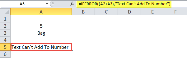
Step 2: To replace the “#VALUE!” error with the text string “text can’t add to number,” enter the following formula in cell A5.
“=IFERROR((A2+A3),”Text Can’t Add to Number”)”
Press the “Enter” key. The output of the IFERROR formula is shown in cell A5 of the following image.
The IFERROR function checks the first argument (A2+A3) for an error. Since this argument does evaluate to an error, the function returns the second argument (text can’t add to number). The text string “text can’t add to number” implies that a text value cannot be added to a numeric value.
Had there been a number in place of the string “bag,” the IFERROR function would have returned the sum of the two numbers.
Hence, since the given values could not be added, the resulting “#VALUE!” error has been replaced by a custom message (text can’t add to number).
Likewise, the IFERROR function can be used for managing errors in Excel. Moreover, the output to be returned (in case of an error) can be customized as per the requirements of the user.
Frequently Asked Questions
1. Define the IFERROR function of Excel.
The IFERROR function detects and handles the various types of Excel errors like “#N/A,” “#DIV/0!,” “#REF!,” “#VALUE!,” and so on. In place of these errors, the function returns a text message, number, empty string, logical value, etc.
The syntax of the IFERROR function of Excel is stated as follows:
“IFERROR(value,value_if_error)”
The first argument “value” is checked for errors. The second argument, “value_if_error,” is returned in case an error is found in the first argument. Both the arguments of the IFERROR function are mandatory.
2. When is the IFERROR function used and how does it work in Excel?
The IFERROR function is used in the following situations:
a. To capture the error and notify its presence to the user
b. To tell Excel what is to be done in case the first argument runs into an error
c. To replace the error with a customized message
The IFERROR function works as follows:
a. The function checks the first argument for errors.
b. In case the first argument does evaluate to an error, the function returns a predefined response. This response is entered as the second argument in the function.
c. In case the first argument does not run into an error, the function returns the result of the first argument.
3. How does the IFERROR function return a blank cell in Excel?
To return a blank cell, an empty string needs to be entered in the second argument of the IFERROR function. For example, two cells contain the following values:
• Cell A1 contains 20
• Cell A2 contains 0
Enter the formula “=IFERROR(A1/A2,””) in cell B1. After pressing the “Enter” key, it returns an empty cell (B1).
As long as cell A2 contains zero, the given IFERROR formula returns a blank cell. This is because the formula identifies division by zero as an error. The moment a value is entered in cell A2, the IFERROR formula returns the result of A1/A2.
Had A1 been a blank cell and A2 contained 20, the formula “=IFERROR(A1/A2,“no message”) would have returned 0. This is because the formula does not identify a blank cell in the numerator as an error. Hence, it returns the result of the first argument.
Recommended Articles
This has been a guide to IFERROR Excel function. We discuss how to handle excel errors (#DIV/0, #N/A, #NAME?, #NULL!, #NUM!, #REF!, #VALUE!,) with examples. You may also look at these useful functions of Excel –
- IFERROR with VLOOKUP in ExcelIFERROR is an error-handling function and Vlookup is a referencing function. They’re combined and used so that when Vlookup encounters an error while finding or matching the data, the formula must know what to do. Vlookup function is nested in the iferror function.read more
- VBA IFERRORThe IFERROR function in Excel is used to determine what to do when an error occurs before performing any function.read more
- VLOOKUP Errors
- ISERROR in ExcelISERROR is a logical function that determines whether or not the cells being referred to have an error. If an error is found, it returns TRUE; if no errors are found, it returns FALSE.read more
Функция ФОШ возвращает функцию ошибки, проинтегрированную от значения аргумента «нижний_предел» до значения аргумента «верхний_предел».
Описание функции ФОШ
Возвращает функцию ошибки, проинтегрированную от значения аргумента «нижний_предел» до значения аргумента «верхний_предел».
Синтаксис
=ФОШ(нижний_предел; [верхний_предел])Аргументы
нижний_пределверхний_предел
Обязательный аргумент. Нижний предел интегрирования ФОШ.
Необязательный аргумент. Верхний предел интегрирования ФОШ. Если аргумент «верхний_предел» опущен, функция ФОШ выполняет интегрирование в пределах от 0 до значения аргумента «нижний_предел».
Замечания
- Если аргумент «нижний_предел» не является числом, функция ФОШ возвращает значение ошибки #ЗНАЧ!.
- Если аргумент «верхний_предел» не является числом, функция ФОШ возвращает значение ошибки #ЗНАЧ!.
Пример
Функция ERF возвращает функцию ошибки, интегрированную между нижним_пределом и верхним_пределом.

Синтаксис
=ERF (lower_limit, [upper_limit])
аргументы
- Нижний предел (обязательно): Нижний предел интегрирования.
- Верхний предел (необязательно): Верхний предел интегрирования. Если опущено, будет возвращена интеграция между 0 и нижним_пределом.
Возвращаемое значение
Функция ERF возвращает числовое значение.
Примечания к функциям
- Функция ERF была улучшена в Excel 2010, и теперь она может вычислять отрицательные значения.
В Excel 2007 функция ERF принимает только положительные значения. Если какой-либо из предоставленных аргументов имеет отрицательное значение, функция ERF вернет ошибку #ЧИСЛО! значение ошибки. - Значение! значение ошибки возникает, если какой-либо из предоставленных аргументов не является числовым.
- Когда верхний_предел опущен, ERF интегрируется между нулем (значение нижнего_предела) и нижним_пределом (значение верхнего_предела). Следовательно, когда нижний предел положительный, ERF возвращает положительный результат. Наоборот.
Более того, когда нижний_предел больше верхнего_предела, ERF возвращает отрицательный результат. Наоборот. - Результирующий диапазон, возвращаемый функцией ERF, находится между -1 и 1.
- Уравнение функции ошибки:


Примеры
Пример первый: результат без верхнего предела
В этом случае мы хотим вычислить функцию ошибки, когда аргумент upper_limit опущен. Это означает, что функция ERF интегрируется между нулем и нижним_пределом. Пожалуйста, сделайте следующее.
1. Пожалуйста, скопируйте приведенную ниже формулу в ячейку E5, затем нажмите клавишу Enter, чтобы получить результат.
=ERF (B5)
2. Выберите эту ячейку результатов и перетащите ее маркер автозаполнения вниз, чтобы получить остальные результаты.

Заметки:
- Как показано на приведенном выше снимке экрана, когда единственный аргумент нижний_лимит отрицательный, возвращаемый результат также отрицательный. Наоборот.
- Когда единственный аргумент нижний_предел равен нулю (0), ERF возвращает в качестве результата ноль (0).
- Аргумент в каждой из приведенных выше формул предоставляется в виде ссылки на ячейку, содержащей числовое значение.
- Мы также можем напрямую ввести значение в формулу. Например, формулу в ячейке E5 можно изменить на:
=ERF (-1)
Пример второй: результат с верхним пределом
В этом случае мы хотим вычислить функцию ошибки, когда предоставлены аргументы lower_limit и upper_limit. Пожалуйста, сделайте следующее.
1. Пожалуйста, скопируйте приведенную ниже формулу в ячейку F5, затем нажмите клавишу Enter, чтобы получить результат.
=ERF (B5, C5)
2. Выберите эту ячейку результатов и перетащите ее маркер автозаполнения вниз, чтобы получить остальные результаты.

Заметки:
- Как видно из приведенного выше снимка экрана, когда верхний_предел больше нижнего_предела, ERF возвращает положительный результат. Наоборот.
- Аргументы в каждой из приведенных выше формул предоставляются в виде ссылок на ячейки, содержащих числовые значения.
- Мы также можем напрямую вводить значения в формулу. Например, формулу в ячейке F5 можно изменить на:
=ERF (-1, 0)
Относительные функции:
-
Excel EVEN Функция
Функция EVEN округляет числа от нуля до ближайшего четного целого числа.
-
Excel EXP Функция
Функция EXP возвращает результат возведения константы e в энную степень.
Лучшие инструменты для работы в офисе
Kutools for Excel — Помогает вам выделиться из толпы
Хотите быстро и качественно выполнять свою повседневную работу? Kutools for Excel предлагает 300 мощных расширенных функций (объединение книг, суммирование по цвету, разделение содержимого ячеек, преобразование даты и т. д.) и экономит для вас 80 % времени.
- Разработан для 1500 рабочих сценариев, помогает решить 80% проблем с Excel.
- Уменьшите количество нажатий на клавиатуру и мышь каждый день, избавьтесь от усталости глаз и рук.
- Станьте экспертом по Excel за 3 минуты. Больше не нужно запоминать какие-либо болезненные формулы и коды VBA.
- 30-дневная неограниченная бесплатная пробная версия. 60-дневная гарантия возврата денег. Бесплатное обновление и поддержка 2 года.
")
Вкладка Office — включение чтения и редактирования с вкладками в Microsoft Office (включая Excel)
- Одна секунда для переключения между десятками открытых документов!
- Уменьшите количество щелчков мышью на сотни каждый день, попрощайтесь с рукой мыши.
- Повышает вашу продуктивность на 50% при просмотре и редактировании нескольких документов.
- Добавляет эффективные вкладки в Office (включая Excel), точно так же, как Chrome, Firefox и новый Internet Explorer.
")
Комментарии (0)
Оценок пока нет. Оцените первым!
IFERROR function provides a great way to handle errors in Excel formulas. Excel IFERROR function returns a custom result (which can be a text, cell reference, or another formula) when the expression enclosed inside it returns an error.
IFERROR helps you catch and address problems with your formulas so you can have clean and orderly spreadsheets. Alternatively, you can use nested IF statements to handle formula errors but nested IF statements are quite challenging to read and reduce the spreadsheets’ maintainability. This is the reason IFERROR function is preferred for handling errors.

Now, let’s see the syntax of the IFERROR function.
Syntax
The syntax of an IFERROR function is as follows:
=IFERROR(value, value_if_error)
'value' – This a required parameter that tells the function what to check for errors. It may be an expression, formula, or cell reference.'value_if_error' – This is also a required parameter that represents the value returned from the function in case of an error. It may be an empty string, a cell reference blank cell, a line of text, a numeric value, or another formula or expression.
Important Characteristics of the IFERROR function
- The IFERROR function deals with all types of errors. This includes #N/A, #DIV/0, #NAME, #NUM!, #NULL, #VALUE, and #REF.
- IFERROR function is only available in Excel 2007 or higher versions.
- To catch errors in earlier versions of Excel (2003 and below), you’ll have to use the ISERROR function combined with the IF function.
- An empty
'value'parameter will result in an empty string («») instead of an error. - An empty
'value_if_error'parameter will also be evaluated as an empty string («»), and hence, no message will be displayed if an error is found. - IFERROR function can be used with array formulas. If an array formula is passed as a value parameter to the IFERROR function, the function returns an array of results for every cell in the specified range.
Types of Formula Errors in Excel
Before going any further, let’s see what all errors can excel formulas throw.
#N/A Error
The #N/A Error stands for Not Available Error. It is thrown when something that you were looking for is not found. Despite its obvious unpleasantness, it is a «useful» error because it tells you something important is missing in your formula.
It may also be triggered by an extra space between characters, wrong spellings, or inconclusive lookup tables. The functions most likely to give you a #N/A error include MATCH, LOOKUP, VLOOKUP, and HLOOKUP.
#DIV/0! Error
The #DIV/0 Error is another type of error often found in Excel. You will find this error every time a number is divided by zero (0) or an empty cell reference. It occurs when you attempt to perform calculations like 10/0.
In many situations, the #DIV/0 error is unavoidable. This is especially true if you prefer to assign formulas before populating your excel worksheets with data. In such situations, you probably don’t want to see an error message at all, and this can be achieved by the IFERROR function.
#VALUE! Error
The #VALUE Error is encountered when you use an incorrect datatype parameter in a formula. It’s Excel’s way of saying there is something wrong with the way you’ve typed your formula. Or that it has identified a problem with the cells you’re attempting to reference.
This error-type is very broad, and it may be hard to determine its exact cause.
Pro tip – While building a formula, you must make sure that the datatypes of all the values involved are compatible. Otherwise, you will encounter this error.
#REF! Error
The #REF! Error, also known as the reference error, is encountered when a reference in a formula has expired. Most commonly, this is the case when a formula points to a cell reference that does not exist (for example, you deleted a row or a column that was being referenced by a formula).
#NAME ERROR
This error commonly occurs as a result of misspelled functions. Unlike word, Excel demands you to type in the exact name of the function you are going to use.
If, for example, you wanted to type HLOOKUP but type HLOKUP instead, you’ll get a #Name error. It means part of your formula needs fixing. Most times, you can avoid it by using the formula wizard.
#NUM ERROR
The #NUM Error occurs when the value you are trying to calculate is beyond Excel’s limits. There are various conditions in which the #NUM Error can occur.
Another scenario that can return a #Num error is when you try to provide a non-numeric value (or any invalid value) to a function argument that only supports numeric values. For example – trying to calculate the square root of a negative number SQRT(-10) will return a #NUM error.
Recommended Reading: Excel ERROR.TYPE Function
Examples of IFERROR Function
Now let’s try to understand the IFERROR function with some examples.
Example 1 – Handling #NA errors in VLOOKUP Function
Let’s assume we have a list of students along with their registration numbers. We try to find the registration number for a student with the name «Glen» out of that list.

For this, we will be writing a VLOOKUP function as –
=VLOOKUP("Glen",A1:B11,2,0)
But since ‘Glen’ doesn’t exist in the student list, so VLOOKUP gives a #N/A error, as shown in the above image.
Now, to replace #N/A with a more meaningful text like «Student Not Found!» we’ll have to use the IFERROR function.
To use the IFERROR function in this case, we will need to use the VLOOKUP function as the first parameter to the IFERROR and text «Student Not Found!» as the second parameter.

The formula should look like this:
=IFERROR(VLOOKUP("Glen",A1:B11,2,0),"Student Not Found!")
Example 2 – Handling #VALUE! Or Invalid Parameter Errors
Let’s assume we have a task planner spreadsheet that calculates the days between two dates using the NETWORKDAYS function as shown.

As shown in the image, Task – 4 is an ongoing task and does not have an enddate, and hence the enddate is marked as ‘NA’. But while calculating days, NETWORKDAYS displays a #VALUE! error.
To fix this error, we can wrap our formula inside an IFERROR function and display a suitable message instead of an error.

So, our formula would be:
=IFERROR(NETWORKDAYS(B6,C6), "Ongoing Task")
Example 3 – Handling #DIV/0! Or Divide By Zero Errors
Now let’s suppose we have a weekly sales stats report of a gift store. The report represents total orders generated by each sales manager along with the total sales value.

In the report, we want to calculate the ‘Average Order Value’ generated by each sales manager. For calculating the ‘average order value’, we can use a formula – Total Sales Value / Total Orders.
An excel formula can represent this as:
=C3/B3
As we can see, the report sales manager ‘Donald Perkins’ has made zero sales for the week, and hence this formula results in an error.
The #DIV/0 error really stands out, and it would be embarrassing to have such errors appear in your excel report.
We can use the IFERROR function in such a case and pass our existing formula as the first argument to the function, and the second argument would be a suitable message or an empty string.

So, the final formula would be:
=IFERROR(C3/B3,"")
This will show an empty string in case an error occurs in the inner formula.
Example 4 – Handling Errors In Array Formulas Using IFERROR Function
Array formulas in excel allow you to perform powerful calculations on one or more value sets. Let’s take example 3 and use an array formula to populate ‘Average Order Value’ against each row.
To do this, we will have an array formula that divides each value in the cell range C3:C7 by the appropriate cell within the range B3:B7, and then press ‘control + shift + enter’ keys.

The formula would be:
{=C3:C7/B3:B7}
And as we can see with the array formula, we are again getting a ‘# DIV/0’ error for the D6 cell.
To fix this, we can use the IFERROR function. IFERROR function, when used with an array formula, returns an array of values for each cell in the range provided.
So our final formula would be:
{=IFERROR(C3:C7/B3:B7,"")}

This formula divides each value in the range C3:C7 with an appropriate value from range B3:B7, and then returns an array of results. The IFERROR function captures all the #DIV/0 errors and replaces them with empty strings.
Example 5 – Importance of IFERROR Function in Excel Calculators and Templates
Let’s consider you are building a Monthly Loan Repayment Calculator in Excel, as shown below.

This template works nicely with all the data, but if the user forgets to enter any mandatory value, the formula returns an error.

Errors like this stand out, and it is quite awkward to have such errors in your excel templates.

To fix this, you could wrap your formulas in an IFERORR function and display a more meaningful message to the end-user. For example:
=IFERROR(PMT((B4%/12),B5,B3,0), "Mandatory fields should not be blank!")
IFERROR vs. ISERROR
The ISERROR function is an error-handling alternative for those who are working with Excel 2003 or lower versions. Since the IFERROR function came out with Excel 2007 so before that, for handling formula errors, we used ISERROR Function with Excel IF Statement.
ISERROR function accepts a single argument, which can be an expression, formula, or cell reference. If the supplied argument results in an error, it returns TRUE otherwise, it returns FALSE.
The errors that the ISERROR function checks are as follows:
- #N/A Error
- #VALUE Error
- #REF Error
- #DIV/0! Error
- #NUM! Error
- #NAME? Error
- #NULL! Error
ISERROR Function differs from the IFERROR in the sense that – the ISERROR function returns a Boolean value if there is an error or not. On the other hand, the IFERROR function allows the user to put up a custom and meaningful value or string instead of the error.
Syntax of ISERROR Function
The syntax of the ISERROR function is as follows:
=ISERROR(value)
'value' – This a required parameter that tells the function what to check for errors. It may be an expression, formula, or cell reference.
ISERROR Function Example
Let’s again revisit Example 1 and try to handle the error using the ISERROR function. So, we have a list of students along with their registration numbers. We try to find the registration number for a student with the name «Glen» out of that list.
For this, we will be writing a VLOOKUP function as –
=VLOOKUP("Glen",A1:B11,2,0)
But since ‘Glen’ doesn’t exist in the student list, so VLOOKUP gives a #N/A error, as shown in the above image. In the previous example, we used the IFERROR function to replace the #N/A error with a more meaningful text like «Student Not Found!»
But here, let’s try to use the ISERROR function along with the IF function to achieve the same result. So, the formula would be:

=IF(ISERROR(VLOOKUP("Glen",A2:B11,2,0)),"Student Not Found!", VLOOKUP("Glen",A2:B11,2,0))
NOTE: IFERROR function automatically assumes you will always want the result if your calculations don’t have any errors. ISERROR, on the other hand, gives you either «TRUE» or a «FALSE», and when combined with the IF function, you can have more control over the result in both outcomes.
Recommended Reading: Excel ISERR Function – How to Use
IFERROR vs. IFNA
IFNA Function is another error handling function in Excel. However, the IFNA function only catches #N/A errors and allows us to display more meaningful error messages in case of a #N/A error.
Syntax of IFNA Function
The syntax of IFNA Function is as follows:
=IFNA(value, value_if_na)
'value' – the expression, formula, or reference excel should be checked for errors.
'value_if_na' – represents the value returned from the function in case of an #N/A error. It may be an empty string, a cell reference blank cell, a line of text, a numeric value, or another formula or expression.
IFNA works best with lookup functions such as VLOOKUP, MATCH, HLOOKUP, and LOOKUP.
IFNA Function Example
Let’s try to understand the IFNA function again with Example 1.
So, we have a list of students, and we are trying to fetch details for a student named «Glen» using a VLOOKUP function. However, since «Glen» is not a part of the list, so the VLOOKUP function throws a #N/A error.

To handle such errors, we make use of the IFNA function as –
=IFNA(VLOOKUP("Glen",A2:B11,2,0),"Student Not Found!")
This formula results in a more meaningful text, «Student Not Found!» if no student with the name «Glen» is found in the given range.
Please Note: IFNA Function only handles #N/A errors and does not catch or handle any other errors, as shown in the below screenshot.

In the above image, we can clearly see that the IFNA function misses the #DIV/0! Error and returns the error as it is.
Recommended Reading: ISNA Function In Excel
So this was all about the IFERROR function in excel. We will get back to you with another amazing function. Stay Tuned!