
So, you have decided that time has come to become an Excel Master. Congratulations!
Before you start with Excel functions and tools, there are some basics that need to be covered first.
Let’s start our magical journey in Excel together! 🙂
A really quick intro to Excel
Excel is the world’s most popular spreadsheet software, developed by Microsoft.
Excel debuted on September 30, 1985, and since that day, kept evolving to meet the requirements of the spreadsheet community.
Most of the Excel versions require installation on your local computer. However, In recent years, Excel can be used online, via Excel Online!
And the best thing? Excel Online is absolutely free.
This website utilizes the technology of Excel Online to help you learn and practice Excel without the need have Excel installed on your computer. Thanks Microsoft! 🙂
So, let’s finish with the talking and start practicing!
Typing in Excel
Excel can be used for complex calculations, but you can always use it to type regular text, just like you’d do in Word or any other software.
All you have to do is select one of the cells and start typing…
You can start by typing your name, your favorite pet, your favorite movie and your lucky number 🙂
When you finish typing, hit the Enter key to exit the cell edit mode.
As you can see, you can type both text and numbers in Excel.
Did you notice that certain parts of the sheets changed after you typed your details? This was done using Excel formulas, which we will cover in the next tutorials 🙂
How does Excel work?
Let’s discuss some of the basic ideas in Excel:
- Excel Cell
- Excel Range
- Excel Worksheet
- Excel Workbook
1. Excel Cell
The Excel Cell is the smallest unit in Excel. The cell is used to store data.
In the previous example, we typed our names and favorite pets, movies and numbers in different Excel Cells.
Excel is comprised of rows and columns. The rows are represented as numbers, and the columns – as letters.
In order to reference a specific cell in Excel, we will type its column letter, followed by the row number.
So, A1 will be the first cell in your worksheet – It’s in the first column (A), and in the first row (1):

Ok, now let’s practice… Type your First Name in cell C3, and your Last Name in cell C4
2. Excel Range
The Excel Range is comprised of two or more adjacent cells. These cells can be in the same row, the same column, or even in multiple rows and columns!
Each range is represented by two cells – The top-left cell, and the bottom-right cell, separated with colons.
For example, Range A3:E7 consists of the following cells:

Now, it’s your time to play with Excel ranges!
3. Excel Worksheet
The Excel Worksheet is comprised of rows and columns.
The default Excel Worksheet contains 1,048,576 rows and 16,384 columns.
In the following example, we have 4 different worksheets:

Tip – We can quickly navigate between worksheets using the shortcut Ctrl+Page Up/Ctrl+Page Down. Click here for more useful Excel shortcuts!
4. Excel Workbook
The Excel file is also called Excel Workbook. It contains one or more worksheets.
The default Excel file type has an XLSX suffix.
Excel allows the user to use data from one worksheet in another worksheet in the same workbook. It also allows connecting between different workbooks.
Basic Calculations with Excel
OK, let’s start with the fun part!
We can perform calculations in Excel easily.
In order to start a calculation in a cell, we will type the = sign (equals), and then type our calculation.
These are the basic operators which can be used:
+ Add
– Substract
/ Divide
* (Asterisk) Multiply
^ Power
So, let’s say we want to find the result of 2+2:

Ok, now let’s practice!
Cell References
Okay, now that we know how to perform basic calculations, let’s learn how we can use cell references to make our calculations much quicker, and dynamic, as well!
If we type the = (equals) sign, followed by a reference to a cell (either by typing the cell name or clicking it), we can reference the data stored in that cell. We can also perform calculations using this way – Instead of manually typing the numbers, we can just reference the cells containing these numbers!
Let’s see how it works:

You can see in the example above that each time we change the data in the referenced cell – It is automatically reflected in the second cell!
Now, time to play with Excel:
Reusing cell references & using Partial and Absolute References
One of the advantages of using cell references in Excel is that we can reuse cell references in adjacent cells by copying the cell, or by dragging the cell to adjacent cells.
Let’s see how it works:

Sometimes, we would like that a certain reference will not move if we reuse the formula in other cells.
In such cases, we can use an Absolute Reference, by hitting the F4 button (or manually typing the $ signs before the column and/or row – not recommended) after typing the cell reference.
Let’s see this in action:

In certain cases, we might prefer using a Partial Reference rather than an Absolute Reference.
A Partial Reference allows us to keep the same reference only for a part of the cell – either the row or the column.
To use Partial Reference, just hit the F4 button until the deserved result is achieved.
Let’s see how we can do the entire Multiplication Table calculation, using only one formula!

Now you are all set to continue your Excel journey and learn how to use Excel functions and tools. Good luck! 🙂
The truth is: before you go for a job interview, you must have basic knowledge of Microsoft Excel. From an accountant to a receptionist, human resources to administration departments all are using Microsoft Excel.
It is not only limited to large companies, small entrepreneurs and college students are using it for their day-to-day work. That’s something that you can’t skip. To get a job, learning basic Excel tasks (at least some) is a must in today’s era, that’s a firm truth.
And, to help you with this I have compiled this guide. This guide will help you to learn all those basics using some examples. And some of the most important beginner’s tutorials.
So without further ado let’s get down to the business.
Introduction to Microsoft Excel
There is a number of spreadsheet programs but of all of them, Excel is the most widely used. People have been using it for the last 30 years and throughout these years, it has been upgraded with more and more features.
The best part about Excel is, that it can apply to many business tasks, including statistics, finance, data management, forecasting, analysis, tracking inventory & billing, and business intelligence. Following are the few things which it can do for you:
- Number Crunching
- Charts and Graphs
- Store and Import Data
- Manipulating Text
- Templates/Dashboards
- Automation of Tasks
- And Much More…
The three most important components of Excel you need to understand first:
1. Cell
A cell is a smallest but most powerful part of a spreadsheet. You can enter your data into a cell either by typing or by copy-paste. Data can be a text, a number, or a date. You can also customize it by changing its size, font color, background color, borders, etc. Every cell is identified by its cell address, cell address contains its column number and row number (If a cell is on the 11th row and on column AB, then its address will be AB11).
2. Worksheet:
A worksheet is made up of individual cells which can contain a value, a formula, or text. It also has an invisible draw layer, which holds charts, images, and diagrams. Each worksheet in a workbook is accessible by clicking the tab at the bottom of the workbook window. In addition, a workbook can store chart sheets; a chart sheet displays a single chart and is accessible by clicking a tab.
3. Workbook
A workbook is a separate file just like every other application has. Each workbook contains one or more worksheets. You can also say that a workbook is a collection of multiple worksheets or can be a single worksheet. You can add or delete worksheets, hide them within the workbook without deleting them, and change the order of your worksheets within the workbook.
Microsoft Excel Window Components
Before you start using it, it’s really important to understand what’s where in its window. So ahead we have all the major components which you need to know before entering the world of Microsoft Excel.

- Active Cell: A cell that is currently selected. It will be highlighted by a rectangular box and its address will be shown in the address bar. You can activate a cell by clicking on it or by using your arrow buttons. To edit a cell, you double-click on it or use F2 as well.
- Column: A column is a vertical set of cells. A single worksheet contains 16384 total columns. Every column has its own alphabet for identity, from A to XFD. You can select a column by clicking on its header.
- Row: A row is a horizontal set of cells. A single worksheet contains 1048576 total rows. Every row has its own number for identity, starting from 1 to 1048576. You can select a row by clicking on the row number marked on the left side of the window.
- Fill Handle: It’s a small dot present in the lower right corner of the active cell. It helps you to fill numeric values, text series, insert ranges, insert serial numbers, etc.
- Address Bar: It shows the address of the active cell. If you have selected more than one cell, then it will show the address of the first cell in the range.
- Formula Bar: The formula bar is an input bar, below the ribbon. It shows the content of the active cell and you can also use it to enter a formula in a cell.
- Title Bar: The title bar will show the name of your workbook, followed by the application name (“Microsoft Excel”).
- File Menu: The file menu is a simple menu like all other applications. It contains options like (Save, Save As, Open, New, Print, Excel Options, Share, etc).
- Quick Access Toolbar: A toolbar to quickly access the options which you frequently use. You can add your favorite options by adding new options to the quick access toolbar.
- Ribbon: Starting from Microsoft Excel 2007, all the options menus are replaced with ribbons. Ribbon tabs are a bunch of specific option group which further contains the option.
- Worksheet Tab: This tab shows all the worksheets which are present in the workbook. By default you will see, three worksheets in your new workbook with the names Sheet1, Sheet2, and Sheet3 respectively.
- Status Bar: It is a thin bar at the bottom of the Excel window. It will give you instant help once you start working in Excel.
Perform Basic Activities (Excel Knowledge Tutorials)
- Add and Delete a Worksheet in Excel
- Add and Remove Hyperlinks in Excel
- Add Watermark in Excel
- Apply Accounting Number Format in Excel
- Apply Background Color to a Cell or the Entire Sheet in Excel
- Delete Hidden Rows in Excel
- Deselect Cells in Excel
- Draw a Line in Excel
- Fill Justify in Excel to Merge Text from Multiple Cells
- Formula Bar in Excel (Hide, Unhide, and Expand)
- Print Excel Gridlines (Remove, Shortcut, & Change Color)
- Add a Button in Excel
- Add a Column in Excel
- Add a Header and Footer in Excel
- Add Page Number in Excel
- Apply Comma Style in Excel
- Apply Strikethrough in Excel
- Convert Negative Numbers into Positive in Excel
- Group Worksheets in the Excel
- Highlight Blank Cells in Excel
- Insert a Timestamp in Excel
- Insert Bullet Points in Excel
- Make Negative Numbers Red in Excel
- Merge – Unmerge Cells in Excel
- Rename Sheet in Excel
- Select Non-Contiguous Cells in Excel
- Show Ruler in Excel
- Spell Check in Excel
- Fill Handle in Excel
- Format Painter in Excel
- Move a Row and Column in Excel
- Excel Options (Mac and Windows)
- Add Border in Excel
- Change Border Color in Excel
- How to Change Column Width in Excel
- Clear Formatting in Excel
- View Two Sheets Side by Side in Excel
- Increase and Decrease Indent in Excel
- Insert an Arrow in a Cell in Excel
- Quick Access Toolbar in Excel
- Remove Pagebreak in Excel
- Rotate Text in Excel (Text Orientation)
- Row Vs Column in Excel (Difference)
- Automatically Add Serial Numbers in Excel
- Insert Delta Symbol in Excel in a Cell
- Insert (Type) Degree Symbol in Excel
- Top 10 Benefits of Microsoft Excel
- Set Print Area in Exm,cel
- Delete Blank Rows in Excel
- Convert a Formula to Value in Excel
- Excel for Accountants
- Sort By Date, Date, and Time & Reverse Date Sort in Excel
- Find and Replace in Excel
- Status Bar in Excel
- Make a Paragraph in a Cell in Excel
- Cell Style (Title, Calculation, Total, Headings…) in Excel
- Hide and Unhide a Workbook in Excel
- Change Date Format in Excel
- Center a Worksheet Horizontally and Vertically in Excel
- Make a Copy of the Excel Workbook (File)
- Write (Type) Vertically in Excel
- Insert Text Box in Excel
- Change Tab Color in Excel (Worksheet Tab Background Color)
- Delete a Single Row or Multiple Rows in Excel
- Copy and Paste a Column in Excel
- Zoom In or Zoom Out in Excel
- Copy Formatting in Excel
- How to Dialog Box in Excel
- How to Freeze Panes in Excel
- Insert a Check Mark Symbol [Tickmark] in Excel
- Quickly Swap Two Cells in Excel
Keyboard Shortcuts for Excel
Following are some of the useful keyboard shortcuts that you learn to perform activities quickly.
- Absolute Reference (Excel Shortcut)
- Add Column (Excel Shortcut)
- Add Comments (Excel Shortcut)
- Add Indent (Excel Shortcut)
- Add New Sheet (Excel Shortcut)
- Align Center (Excel Shortcut)
- Apply Border (Excel Shortcut)
- Apply and Remove Filter (Excel Shortcut)
- Auto Fit (Excel Shortcut)
- AutoSum (Excel Shortcut)
- Check Mark (Excel Shortcut)
- Clear Contents (Excel Shortcut)
- Close (Excel Shortcut)
- Copy and Paste (Excel Shortcut)
- Currency Format (Excel Shortcut)
- Cut and Paste (Excel Shortcut)
- Delete Cell (Excel Shortcut)
- Delete Row(s) (Excel Shortcut)
- Delete Sheet (Excel Shortcut)
- Drag Down (Excel Shortcut)
- Edit Cell (Excel Shortcut)
- Fill Color (Excel Shortcut)
- Find and Replace (Excel Shortcut)
- Format Painter (Excel Shortcut)
- Freeze Pane (Excel Shortcut)
- Full Screen (Excel Shortcut)
- Group (Excel Shortcut)
- Hyperlink (Excel Shortcut)
- Insert Cell (Excel Shortcut)
- Insert – Add Row(s) (Excel Shortcut)
- Lock Cells (Excel Shortcut)
- Merge-Unmerge Cells (Excel Shortcut)
- Open Format Cells Option (Excel Shortcut)
- Paste Values (Excel Shortcut)
- Percentage Format (Excel Shortcut)
- Print Preview (Excel Shortcut)
- Save As (Excel Shortcut)
- Select Row (Excel Shortcut)
- Show Formulas (Excel Shortcut)
- Strikethrough (Excel Shortcut)
- Subscript (Excel Shortcut)
- Superscript (Excel Shortcut)
- Switch Tabs (Excel Shortcut)
- Transpose (Excel Shortcut)
- Undo and Redo (Excel Shortcut)
- Unhide Columns (Excel Shortcut)
- Wrap Text (Excel Shortcut)
- Zoom-In (Excel Shortcut)
- Apply Date Format (Excel Shortcut)
- Apply Time Format (Excel Shortcut)
- Delete (Excel Shortcut)
- Open Go To Option (Excel Shortcut)
- Excel Date Functions
- Excel Financial Functions
- Excel Information Functions
- Excel Logical Functions
- Excel Lookup Functions
- Excel Math Functions
- Excel Statistical Functions
- Excel String (Text) Functions
- Excel Time Functions
- INT
- SUMPRODUCT
- MROUND
- MOD
- SUMIFS
- ABS
- SUMIF
- What is a Function in Excel
Recommended Books
Below are my two favorite Excel books for beginners which every person who is starting out with Excel should read.
- Excel 2016 for Dummies: This book covers everything you need to know to perform the task at hand. Includes information on creating and editing worksheets, formatting cells, and entering formulas […]
- Microsoft Excel 2016 Bible: Whether you are just starting out or an Excel novice, the Excel 2016 Bible is your comprehensive, go-to guide for all your Excel 2016 needs Whether you use Excel at work or […]
From Excel Basics to Advanced with In-Depth Guides and Tutorials
- Excel Formulas
- Pivot Table
- Excel Functions
- Power Query
- Excel for Accountants
- Benefits of Microsoft Excel
- VBA in Excel
- Excel Skills
Learning Objectives:
- Why Excel?
- Basic Excel
- Worksheet Functions
What is Excel? Why Excel?
Excel is a spreadsheet program. It is widely used in the industry because they are simple, and also allow you to view data visually.
Since Excel is widely used, it is usually the basic requirement for many jobs.
Here, we will go into the basics of Excel, and how to use them.
Cells
The basic element of spreadsheet is a cell. We often work with multiple cells. Some cells will be data, some cells will be calculation steps and some cells contains results that require calculations.
Another cell in the same sheet
The first thing to learn in excel is how to refer to another cell. There are 2 ways to reference cells:
- A1 method and
- R1C1 method.
The A1 method is more commonly used, since the columns are already labeled with letters, and the rows are labeled by numbers.
However, if your dataset has many columns (more than 26), it might be a good idea to use the R1C1 method.
To calculate the sum of 2 cells A1 and B1, simply type in the equation box:
= A1 + B1.
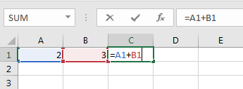
Pressing the Enter key will then give you the following result.
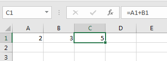
This is assuming that both A1 and B1 contain numerical values. Otherwise, you will get a #VALUE! Error.
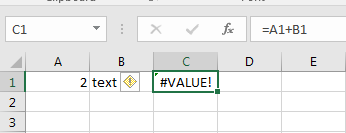
If you place your mouse cursor on the yellow diamond box, it will tell you what error has occurred.
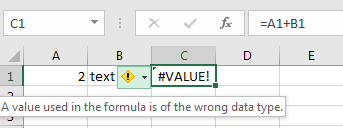
Because A1 contains a numerical value, and B1 contains text, you cannot apply the Sum function, hence Excel raises an error.
We then show an example of multiplication as below.
Range, Worksheet and Workbook
We sometimes need to refer to a group of cells for calculation. Range is always rectangular, hence, we just need the top left cell and bottom right cell. For example, A1:B2 implies cells A1, A2, B1, and B2.
To refer to cells in other worksheet in the same workbook (xlsx file), we use the name and exclamation mark. For example, =Sheet1!A1
To refers to cells in the other worksheet in the different workbook, we use squared bracket. For example, =[appl.xlsx]Sheet1!A1 for workbook that is currently open in Excel. Alternatively, ='C:\document\[appl.xlsx]'Sheet1!A1 for workbook that is not open.
Copy and Paste: Iteration
Copy and Paste is the most commonly used operation in Excel. It is very powerful tools to perform calculation repetitively. In programming terminology, it is called iteration.
Referencing: Absolute vs. Relative
You can use absolute referencing, or relative referencing. We start by explaining relative referencing.
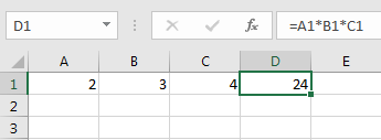
Say I have the following values for columns A, B, and C, and I want to calculate D as their product. If I simply copy D1 and paste it in D2, by default Excel will take it as relative referencing, and D2 = A2*B2*C2 = 210.
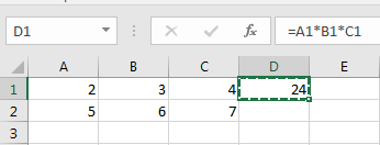

What if I want to reuse the value of A1, say I want D2 = A1*B2*C2? We then use the $ sign to indicate absolute referencing. Placing the $ sign in front of the row or column of the cell will tell Excel to always take that particular row or column even when the formula is copied.
Tips: Pressing F2 will change between relative address and absolute address.


We see that D2=A1*B2*C2 even when we copied the formula from D1. Because of the $ in $A$1, Excel did not use relative referencing for that row/column.
The following example shows how relative address can be used effectively to reduce typing when we create multiplication table. We just need to enter the formula in B2. Then copy and paste the rest of the cells.
| A | B | C | |
|---|---|---|---|
| 1 | x | 1 | 2 |
| 2 | 1 | =$A2*B$1 |
|
| 3 | 2 |
Naming
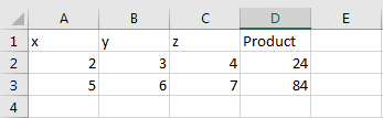
Usually, we will label our rows and/or columns, to let the user know what kind of data or variables are in the spreadsheet. This is for convenience so that the user can follow what you are doing easily.
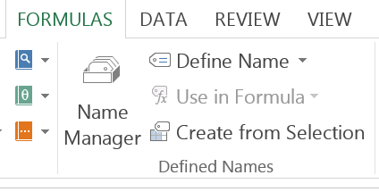
Moreover, we give a name to a cell. In the ribbon, choose FORMULAS tab and then choose to define the name. Then you can refer a cell by its name. This is particularly useful to make your spreadsheet easy to read and understand by other users.
dividend discount model
Let us illustrate the idea of relative address using the dividend discount model(DDM) example. Consider stock which pays out a fixed dividend of $1 per year for the next 10 years. The rate of inflation is going to be constant at 3% per year. We want to find out how much the future dividend payouts are worth in present values.
The discount factor is equal to 1/1.03, which is approximately 0.9709. How do we do this calculation efficiently in Excel? We make use of both relative and absolute referencing.
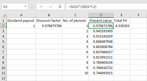
The only thing that changes here is the overall discount factor, which depends on the number of years ahead. Hence we use absolute referencing for the dividend payout amount, and the yearly discount factor, and then multiply the yearly discount factor accordingly with the number of years. Lastly, we sum up the values to get 8.53.
Worksheet Functions
Excel spreadsheet is very convenient because it has a large number of built-in functions that perform calculation without programming. We will learn how to write these functions by yourself in the next class using VBA.
Arithmetic Operators
We first cover some basic arithmetic operators and some basic mathematics functions.
| Function | Meaning |
|---|---|
+ |
Addition |
- |
Substraction |
* |
Multiplication |
/ |
Division |
^ |
Power |
| SQRT() | Square Root |
| ABS() | Absolute number |
Basic Math Functions
| Function | Meaning |
|---|---|
| COUNT(range) | Counts the number of cells in a range that contain numbers |
| SUM(range) | Adds all the numbers in a range of cells |
| PRODUCT(range) | Multiplies all the numbers given as arguments |
| SUMPRODUCT(range1, range2) | Sum of products of the first elements in both ranges, the second elements,…. |
Basic Statistic Functions
| Function | Meaning |
|---|---|
| MIN(range) | Returns the smallest number in a set of values. Ignores logical values and text |
| MAX(range) | Returns the largest number in a set of values. Ignores logical values and text |
| MEDIAN(range) | Returns the median, or the number in the middle of the set of given numbers |
| VAR.P(range) | Calculates population variance |
| VAR.S(range) | Calculates sample variance |
| STDEV.P(range) | Calculate population standard deviation |
| STDEV.S(range) | Calculate sample standard deviation |
The following example shows AVERAGE is used to calculate simple moving average.
| A | B | C | |
|---|---|---|---|
| 1 | n | 5 | |
| 2 | beta | =2/(A1+1) |
|
| 3 | Date | Price | SMA(n) |
| 4 | 02-May-16 | 19 | |
| … | |||
| 7 | 06-May-16 | 30 | =AVERAGE(B3:B7) |
| 8 | 07-May-16 | 56 |
The following example shows AVERAGE and recursive formula is used to calculate exponential moving average. Note that initial EMA is SMA. And the recursive formula is $$EMA{t}(n) = beta P{t}(n) + (1-beta) EMA_{t-1}(n)$$
where $beta=2/(n+1)$.
| A | B | C | |
|---|---|---|---|
| 1 | n | 5 | |
| 2 | beta | =2/(A1+1) |
|
| 3 | Date | Price | EMA(n) |
| 4 | 02-May-16 | 19 | |
| … | |||
| 7 | 06-May-16 | 30 | =AVERAGE(B3:B7) |
| 8 | 07-May-16 | 56 | =$B$2*B9+(1-$B$2)*C8 |
Advanced Statistic Functions
| Function | Meaning |
|---|---|
| COVARIANCE.P(range1 ,range2) | Calculate population covariance using data in range 1 and range 2 |
| COVARIANCE.S(range1, range2) | Calculate sample covariance using data in range 1 and range 2 |
| INTERCEPT(yrange,xrange) | Returns the intercept of simple linear regression of y on x |
| SLOPE(yrange, xrange) | Returns the slope of simple linear regression of y on x |
| STEYX(yrange, xrange) | Returns the standard error of simple linear regression of y on x |
| RAND() | Returns a random number greater than or equal to 0 and less than 1, evenly distributed |
| RANDBETWEEN(integer1, integer2) | Returns a random number between integer1 and integer 2 where integer1 is less than integer2 |
| NORM.INV(probability, mean, standard deviation) | Returns the inverse of the normal cumulative distribution at the given probability under the specified mean and standard deviation. |
How to generate normal distribution? We will use a method called inversion. Use RAND to generate uniform distribution and then use NORM.INV is to generate a normal variable.
Lookup
Lookup functions allow you to get data from another table. Two basic lookup functions are VLOOKUP or HLOOKUP. They help to locate particular cells in table. Using MATCH and INDEX together allows us to have a flexible vlookup and hlookup, when we have 2 different types of data.
For example, we could use =INDEX(range1, MATCH(key, range2)).
| Function | Meaning |
|---|---|
| VLOOKUP(key, range, column, FALSE) | Looks for key in the leftmost column of a table (given by the range), and then returns a value in the same row from a column you specify. |
| HLOOKUP(key, range, column, FALSE) | Looks for key in the top row of a table (given by the range) and returns the value in the same column from a row you specify. |
| MATCH(key, range) | This helps you search for a particular value within a dataset. The output returned is the relative position of the value in the dataset, for example, D8. The key is the value that you want to find, and the range is the range of data that you are searching for. |
| INDEX(range, index) | Returns a value or reference of the cell at the intersection of a particular row and column, in a given range. The output will be the content of that particular cell at that index. |
The following example shows how vlookup can be used to merge two tables.
| A | B | C | D | |
|---|---|---|---|---|
| 1 | Stock | Price | Stock | Volume |
| 2 | Apple | 10 | IBM | 10 |
| 3 | IBM | 20 | 20 | |
| 4 | 30 | Apple | 30 | |
| 5 | ||||
| 6 | Stock | Price | Volume | |
| 7 | Apple | =VLOOKUP(A7,$A$1:$B$4,2,FALSE) |
=VLOOKUP(A7,$C$1:$D$4,2,FALSE) |
|
| 8 | IBM | |||
| 9 |
The following example shows how index and match can be used to merge two tables.
| A | B | C | D | |
|---|---|---|---|---|
| 1 | Stock | Price | Stock | Volume |
| 2 | Apple | 10 | IBM | 10 |
| 3 | IBM | 20 | 20 | |
| 4 | 30 | Apple | 30 | |
| 5 | ||||
| 6 | Stock | Price | Volume | |
| 7 | Apple | =INDEX(B2:B4,MATCH(A7, A2:A4,0)) |
=INDEX(D2:D4, MATCH(A7,C2:C4,0)) |
|
| 8 | IBM | |||
| 9 |
Cell Referencing Function
The following cell referencing functions are very useful to make the code clean and tidy. Offset moves the cell reference to another cell or range of cells. Indirect convert text to cell reference and Address convert cell reference to text.
| Function | Meaning |
|---|---|
| OFFSET(cell, row, column,height and width) | Returns a reference to a range that is a given number of rows and columns from a given reference. Cell refers to the reference cell that you are taking reference from. For row, positive values will mean cells downwards from the reference cell, and negative values will mean cells above the reference cell. For column, positive values will mean cells to the right of the reference cell, while negative values will mean cells to the left of the reference cell. |
| INDIRECT(address string) | Returns the reference specified by a text string. One example would be INDIRECT("A1"), which returns the contents of the cell A1. |
| ADDRESS(row, column) | Creates a cell reference as text, given specified row and column numbers. For example, ADDRESS(2, 7) will return $G$2 as output. |
Combination of INDIRECT and ADDRESS is useful if you do not want to type out the address string, or you have very large datasets. We can use INDIRECT(ADDRESS(1,2)).
The following example shows offset can be used to make spreadsheet customization. We consider K-day momentum where K allow the user to input. While OFFSET is rather simple, we need to take care the case when momentum cannot be calculate in the first K days.
| A | B | C | |
|---|---|---|---|
| 1 | K | 5 | |
| 2 | Date | Price | K-Momentum |
| 3 | 02-May-16 | 10 | =IF(COUNT($A$3:A3)>=$B$1+1,B3-OFFSET(B3,-$B$1), "") |
| 4 | 03-May-16 | 9 | |
| 5 | 04-May-16 | 8 |
The following sample shows more advanced use of OFFSET. We consider n-day simple moving average where n allows the user to input. We only start the calculation when on the n-th day.
| A | B | C | |
|---|---|---|---|
| 1 | n | 5 | |
| 2 | Date | Price | SMA(n) |
| 4 | 02-May-16 | 10 | =IF(COUNT($A$3:A3)>=$B$1,average(Offset(B3,0,0,-$B1$)), "") |
| 5 | 03-May-16 | 9 | |
| 6 | 04-May-16 | 8 |
The following sample shows more advanced use of OFFSET. We consider n-day simple moving average where n allows the user to input. We only start the calculation of EMA when on the n-th day. The first EMA is SMA. Then the rest is by the updating recursive formula.
| A | B | C | |
|---|---|---|---|
| 1 | n | 5 | |
| 2 | beta | =2/(A1+1) |
|
| 3 | Date | Price | EMA(n) |
| 4 | 02-May-16 | 19 | =IF(COUNT($A$4:A4)=$B$1,average(Offset(B4,0,0,-$B1$)),IF(COUNT($A$4:A4)>$B$1,=$B$2*B4+(1-$B$2)*C3, "") |
| 5 | 03-May-16 |
Hyperlink
The following function refers the external link. Hyperlink connects to external file or internet address.
| Function | Meaning |
|---|---|
| HYPERLINK(location, text) | Creates a shortcut or jump that opens a document stored on your hard drive, a network server, or on the internet. For location, you could use places on your computer such as Desktop or C:, or use internet address such as http://www.google.com. The text will be shown as a hyperlink, for example, you could put Click to open Google search'. |
Text Function
The following shows some basic text functions. Len is to find the length. Trim and Clean is to clean up the text. Concatenate is to combine text.
| Function | Meaning |
|---|---|
| LEN(text) | Short form for length. Returns the number of characters in a text string. For example, LEN(apple) returns 5. |
| TRIM(text) | Removes all spaces from a text string except for single spaces between words. |
| CLEAN(text) | Removes all nonprintable characters from text. |
| CONCATENATE(text1, text2, …) | Joins all text strings into one text string. For example, CONCATENATE("I am", "a boy", ...) returns I ama boy. Note that space is not automatically added between text. |
There are some advanced text functions: Left, Right and Mid extract part of text. Find and Search are to look for string and Substitute is to replace text.
| Function | Meaning |
|---|---|
| LEFT(text, number) | Returns the specified number of characters from the left of the text string. For example, LEFT("testing", 2) will return you te. |
| RIGHT (text, number) | Returns the specified number of characters from the right of the text string. For example, RIGHT("testing", 2) will return you ng. |
| MID (text, start position, number) | Returns the specified number of characters from the start position of the text string. For example, MID("testing", 3,2) will return you st |
| FIND(text, target) | Returns the starting position of one text string within the target text string. For example, FIND("apple", "I like apple") returns 8. Note that FIND is case-sensitive, meaning that upper-case letters are not the same as lower-case letters. For example, FIND("APPLE", "I like apple") returns an error. |
| SEARCH(text, target) | Same as FIND but not case-sensitive. For example For example, SEARCH("APPLE", "I like apple") returns 8 |
| SUBSTITUTE(target, new text, old text) | Replaces existing text with new text in a text string. For example, SUBSTITUTE("I like apple", "apple", "banana") returns I like banana. |
Время на прочтение
7 мин
Количество просмотров 312K
Приветствую всех.
В этом посте я расскажу, что такое VBA и как с ним работать в Microsoft Excel 2007/2010 (для более старых версий изменяется лишь интерфейс — код, скорее всего, будет таким же) для автоматизации различной рутины.

VBA (Visual Basic for Applications) — это упрощенная версия Visual Basic, встроенная в множество продуктов линейки Microsoft Office. Она позволяет писать программы прямо в файле конкретного документа. Вам не требуется устанавливать различные IDE — всё, включая отладчик, уже есть в Excel.
Еще при помощи Visual Studio Tools for Office можно писать макросы на C# и также встраивать их. Спасибо, FireStorm.
Сразу скажу — писать на других языках (C++/Delphi/PHP) также возможно, но требуется научится читать, изменять и писать файлы офиса — встраивать в документы не получится. А интерфейсы Microsoft работают через COM. Чтобы вы поняли весь ужас, вот Hello World с использованием COM.
Поэтому, увы, будем учить Visual Basic.
Чуть-чуть подготовки и постановка задачи
Итак, поехали. Открываем Excel.
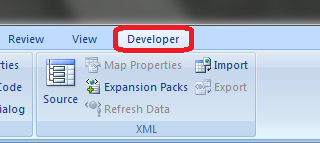
Для начала давайте добавим в Ribbon панель «Разработчик». В ней находятся кнопки, текстовые поля и пр. элементы для конструирования форм.

Появилась вкладка.
Теперь давайте подумаем, на каком примере мы будем изучать VBA. Недавно мне потребовалось красиво оформить прайс-лист, выглядевший, как таблица. Идём в гугл, набираем «прайс-лист» и качаем любой, который оформлен примерно так (не сочтите за рекламу, пожалуйста):

То есть требуется, чтобы было как минимум две группы, по которым можно объединить товары (в нашем случае это будут Тип и Производитель — в таком порядке). Для того, чтобы предложенный мною алгоритм работал корректно, отсортируйте товары так, чтобы товары из одной группы стояли подряд (сначала по Типу, потом по Производителю).
Результат, которого хотим добиться, выглядит примерно так:

Разумеется, если смотреть прайс только на компьютере, то можно добавить фильтры и будет гораздо удобнее искать нужный товар. Однако мы хотим научится кодить и задача вполне подходящая, не так ли?
Кодим
Для начала требуется создать кнопку, при нажатии на которую будет вызываться наша програма. Кнопки находятся в панели «Разработчик» и появляются по кнопке «Вставить». Вам нужен компонент формы «Кнопка». Нажали, поставили на любое место в листе. Далее, если не появилось окно назначения макроса, надо нажать правой кнопкой и выбрать пункт «Назначить макрос». Назовём его FormatPrice. Важно, чтобы перед именем макроса ничего не было — иначе он создастся в отдельном модуле, а не в пространстве имен книги. В этому случае вам будет недоступно быстрое обращение к выделенному листу. Нажимаем кнопку «Новый».


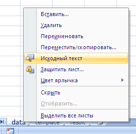
И вот мы в среде разработки VB. Также её можно вызвать из контекстного меню командой «Исходный текст»/«View code».

Перед вами окно с заглушкой процедуры. Можете его развернуть. Код должен выглядеть примерно так:
Sub FormatPrice()End Sub
Напишем Hello World:
Sub FormatPrice()

    MsgBox "Hello World!"

End Sub
И запустим либо щелкнув по кнопке (предварительно сняв с неё выделение), либо клавишей F5 прямо из редактора.
Тут, пожалуй, следует отвлечься на небольшой ликбез по поводу синтаксиса VB. Кто его знает — может смело пропустить этот раздел до конца. Основное отличие Visual Basic от Pascal/C/Java в том, что команды разделяются не ;, а переносом строки или двоеточием (:), если очень хочется написать несколько команд в одну строку. Чтобы понять основные правила синтаксиса, приведу абстрактный код.
Примеры синтаксиса
' Процедура. Ничего не возвращает

' Перегрузка в VBA отсутствует

Sub foo(a As String, b As String)

    ' Exit Sub ' Это значит "выйти из процедуры"

    MsgBox a + ";" + b

End Sub' Функция. Вовращает Integer

Function LengthSqr(x As Integer, y As Integer) As Integer

    ' Exit Function

    LengthSqr = x * x + y * y

End FunctionSub FormatPrice()

    Dim s1 As String, s2 As String

    s1 = "str1"

    s2 = "str2"

    If s1 <> s2 Then

        foo "123", "456" ' Скобки при вызове процедур запрещены

    End IfDim res As sTRING ' Регистр в VB не важен. Впрочем, редактор Вас поправит

    Dim i As Integer

    ' Цикл всегда состоит из нескольких строк

    For i = 1 To 10

        res = res + CStr(i) ' Конвертация чего угодно в String

        If i = 5 Then Exit For

    Next iDim x As Double

    x = Val("1.234") ' Парсинг чисел

    x = x + 10

    MsgBox xOn Error Resume Next ' Обработка ошибок - игнорировать все ошибки

    x = 5 / 0

    MsgBox xOn Error GoTo Err ' При ошибке перейти к метке Err

    x = 5 / 0

    MsgBox "OK!"

    GoTo ne
Err:
MsgBox
"Err!"
ne:
On Error GoTo 0 ' Отключаем обработку ошибок
' Циклы бывает, какие захотите
Do While True
Exit DoLoop 'While True
Do 'Until False
Exit Do
Loop Until False
' А вот при вызове функций, от которых хотим получить значение, скобки нужны.
' Val также умеет возвращать Integer
Select Case LengthSqr(Len("abc"), Val("4"))
Case 24
MsgBox "0"
Case 25
MsgBox "1"
Case 26
MsgBox "2"
End Select' Двухмерный массив.
' Можно также менять размеры командой ReDim (Preserve) - см. google
Dim arr(1 to 10, 5 to 6) As Integer
arr(1, 6) = 8Dim coll As New Collection
Dim coll2 As Collection
coll.Add "item", "key"
Set coll2 = coll ' Все присваивания объектов должны производится командой Set
MsgBox coll2("key")
Set coll2 = New Collection
MsgBox coll2.Count
End Sub
Грабли-1. При копировании кода из IDE (в английском Excel) есь текст конвертируется в 1252 Latin-1. Поэтому, если хотите сохранить русские комментарии — надо сохранить крокозябры как Latin-1, а потом открыть в 1251.
Грабли-2. Т.к. VB позволяет использовать необъявленные переменные, я всегда в начале кода (перед всеми процедурами) ставлю строчку Option Explicit. Эта директива запрещает интерпретатору заводить переменные самостоятельно.
Грабли-3. Глобальные переменные можно объявлять только до первой функции/процедуры. Локальные — в любом месте процедуры/функции.
Еще немного дополнительных функций, которые могут пригодится: InPos, Mid, Trim, LBound, UBound. Также ответы на все вопросы по поводу работы функций/их параметров можно получить в MSDN.
Надеюсь, что этого Вам хватит, чтобы не пугаться кода и самостоятельно написать какое-нибудь домашнее задание по информатике. По ходу поста я буду ненавязчиво знакомить Вас с новыми конструкциями.
Кодим много и под Excel
В этой части мы уже начнём кодить нечто, что умеет работать с нашими листами в Excel. Для начала создадим отдельный лист с именем result (лист с данными назовём data). Теперь, наверное, нужно этот лист очистить от того, что на нём есть. Также мы «выделим» лист с данными, чтобы каждый раз не писать длинное обращение к массиву с листами.
Sub FormatPrice()

    Sheets("result").Cells.Clear

    Sheets("data").Activate

End Sub
Работа с диапазонами ячеек
Вся работа в Excel VBA производится с диапазонами ячеек. Они создаются функцией Range и возвращают объект типа Range. У него есть всё необходимое для работы с данными и/или оформлением. Кстати сказать, свойство Cells листа — это тоже Range.
Примеры работы с Range
Sheets("result").Activate

Dim r As Range

Set r = Range("A1")

r.Value = "123"

Set r = Range("A3,A5")

r.Font.Color = vbRed

r.Value = "456"

Set r = Range("A6:A7")

r.Value = "=A1+A3"
Теперь давайте поймем алгоритм работы нашего кода. Итак, у каждой строчки листа data, начиная со второй, есть некоторые данные, которые нас не интересуют (ID, название и цена) и есть две вложенные группы, к которым она принадлежит (тип и производитель). Более того, эти строки отсортированы. Пока мы забудем про пропуски перед началом новой группы — так будет проще. Я предлагаю такой алгоритм:
- Считали группы из очередной строки.
- Пробегаемся по всем группам в порядке приоритета (вначале более крупные)
- Если текущая группа не совпадает, вызываем процедуру AddGroup(i, name), где i — номер группы (от номера текущей до максимума), name — её имя. Несколько вызовов необходимы, чтобы создать не только наш заголовок, но и всё более мелкие.
- После отрисовки всех необходимых заголовков делаем еще одну строку и заполняем её данными.
Для упрощения работы рекомендую определить следующие функции-сокращения:
Function GetCol(Col As Integer) As String

    GetCol = Chr(Asc("A") + Col)

End FunctionFunction GetCellS(Sheet As String, Col As Integer, Row As Integer) As Range

    Set GetCellS = Sheets(Sheet).Range(GetCol(Col) + CStr(Row))

End FunctionFunction GetCell(Col As Integer, Row As Integer) As Range

    Set GetCell = Range(GetCol(Col) + CStr(Row))

End Function
Далее определим глобальную переменную «текущая строчка»: Dim CurRow As Integer. В начале процедуры её следует сделать равной единице. Еще нам потребуется переменная-«текущая строка в data», массив с именами групп текущей предыдущей строк. Потом можно написать цикл «пока первая ячейка в строке непуста».
Глобальные переменные
Option Explicit ' про эту строчку я уже рассказывал

Dim CurRow As Integer

Const GroupsCount As Integer = 2

Const DataCount As Integer = 3
FormatPrice
Sub FormatPrice()

    Dim I As Integer ' строка в data

    CurRow = 1

    Dim Groups(1 To GroupsCount) As String

    Dim PrGroups(1 To GroupsCount) As String
Sheets(
"data").Activate
I = 2
Do While True
If GetCell(0, I).Value = "" Then Exit Do
' ...
I = I + 1
Loop
End Sub
Теперь надо заполнить массив Groups:
На месте многоточия
Dim I2 As Integer

For I2 = 1 To GroupsCount

    Groups(I2) = GetCell(I2, I)

Next I2

' ...

For I2 = 1 To GroupsCount ' VB не умеет копировать массивы

    PrGroups(I2) = Groups(I2)

Next I2

I =  I + 1
И создать заголовки:
На месте многоточия в предыдущем куске
For I2 = 1 To GroupsCount

    If Groups(I2) <> PrGroups(I2) Then

        Dim I3 As Integer

        For I3 = I2 To GroupsCount

            AddHeader I3, Groups(I3)

        Next I3

        Exit For

    End If

Next I2
Не забудем про процедуру AddHeader:
Перед FormatPrice
Sub AddHeader(Ty As Integer, Name As String)

    GetCellS("result", 1, CurRow).Value = Name

    CurRow = CurRow + 1

End Sub
Теперь надо перенести всякую информацию в result
For I2 = 0 To DataCount - 1

    GetCellS("result", I2, CurRow).Value = GetCell(I2, I)

Next I2
Подогнать столбцы по ширине и выбрать лист result для показа результата
После цикла в конце FormatPrice
Sheets("Result").Activate

Columns.AutoFit
Всё. Можно любоваться первой версией.

Некрасиво, но похоже. Давайте разбираться с форматированием. Сначала изменим процедуру AddHeader:
Sub AddHeader(Ty As Integer, Name As String)

    Sheets("result").Range("A" + CStr(CurRow) + ":C" + CStr(CurRow)).Merge

    ' Чтобы не заводить переменную и не писать каждый раз длинный вызов

    ' можно воспользоваться блоком With

    With GetCellS("result", 0, CurRow)

        .Value = Name

        .Font.Italic = True

        .Font.Name = "Cambria"

        Select Case Ty

        Case 1 ' Тип

            .Font.Bold = True

            .Font.Size = 16

        Case 2 ' Производитель

            .Font.Size = 12

        End Select

        .HorizontalAlignment = xlCenter

    End With

    CurRow = CurRow + 1

End Sub
Уже лучше:

Осталось только сделать границы. Тут уже нам требуется работать со всеми объединёнными ячейками, иначе бордюр будет только у одной:

Поэтому чуть-чуть меняем код с добавлением стиля границ:
Sub AddHeader(Ty As Integer, Name As String)

    With Sheets("result").Range("A" + CStr(CurRow) + ":C" + CStr(CurRow))

        .Merge

        .Value = Name

        .Font.Italic = True

        .Font.Name = "Cambria"

        .HorizontalAlignment = xlCenterSelect Case Ty

        Case 1 ' Тип

            .Font.Bold = True

            .Font.Size = 16

            .Borders(xlTop).Weight = xlThick

        Case 2 ' Производитель

            .Font.Size = 12

            .Borders(xlTop).Weight = xlMedium

        End Select

        .Borders(xlBottom).Weight = xlMedium ' По убыванию: xlThick, xlMedium, xlThin, xlHairline

    End With

    CurRow = CurRow + 1

End Sub

Осталось лишь добится пропусков перед началом новой группы. Это легко:
В начале FormatPrice
Dim I As Integer ' строка в  data

CurRow = 0 ' чтобы не было пропуска в самом начале

Dim Groups(1 To GroupsCount) As String
В цикле расстановки заголовков
If Groups(I2) <> PrGroups(I2) Then

    CurRow = CurRow + 1

    Dim I3 As Integer

В точности то, что и хотели.
Надеюсь, что эта статья помогла вам немного освоится с программированием для Excel на VBA. Домашнее задание — добавить заголовки «ID, Название, Цена» в результат. Подсказка: CurRow = 0 CurRow = 1.
Файл можно скачать тут (min.us) или тут (Dropbox). Не забудьте разрешить исполнение макросов. Если кто-нибудь подскажет человеческих файлохостинг, залью туда.
Спасибо за внимание.
Буду рад конструктивной критике в комментариях.
UPD: Перезалил пример на Dropbox и min.us.
UPD2: На самом деле, при вызове процедуры с одним параметром скобки можно поставить. Либо использовать конструкцию Call Foo(«bar», 1, 2, 3) — тут скобки нужны постоянно.
Excel for Microsoft 365 Excel 2021 Excel 2019 Excel 2016 Excel 2013 Excel 2010 More…Less
Excel is an incredibly powerful tool for getting meaning out of vast amounts of data. But it also works really well for simple calculations and tracking almost any kind of information. The key for unlocking all that potential is the grid of cells. Cells can contain numbers, text, or formulas. You put data in your cells and group them in rows and columns. That allows you to add up your data, sort and filter it, put it in tables, and build great-looking charts. Let’s go through the basic steps to get you started.
Excel documents are called workbooks. Each workbook has sheets, typically called spreadsheets. You can add as many sheets as you want to a workbook, or you can create new workbooks to keep your data separate.
-
Click File, and then click New.
-
Under New, click the Blank workbook.

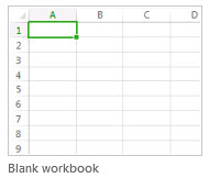
-
Click an empty cell.
For example, cell A1 on a new sheet. Cells are referenced by their location in the row and column on the sheet, so cell A1 is in the first row of column A.
-
Type text or a number in the cell.
-
Press Enter or Tab to move to the next cell.
-
Select the cell or range of cells that you want to add a border to.
-
On the Home tab, in the Font group, click the arrow next to Borders, and then click the border style that you want.
For more information, see Apply or remove cell borders on a worksheet .
-
Select the cell or range of cells that you want to apply cell shading to.
-
On the Home tab, in the Font group, choose the arrow next to Fill Color
, and then under Theme Colors or Standard Colors, select the color that you want.
 , and then under Theme Colors or Standard Colors, select the color that you want.
For more information about how to apply formatting to a worksheet, see Format a worksheet.
When you’ve entered numbers in your sheet, you might want to add them up. A fast way to do that is by using AutoSum.
-
Select the cell to the right or below the numbers you want to add.
-
Click the Home tab, and then click AutoSum in the Editing group.
AutoSum adds up the numbers and shows the result in the cell you selected.
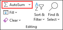
For more information, see Use AutoSum to sum numbers
Adding numbers is just one of the things you can do, but Excel can do other math as well. Try some simple formulas to add, subtract, multiply, or divide your numbers.
-
Pick a cell, and then type an equal sign (=).
That tells Excel that this cell will contain a formula.
-
Type a combination of numbers and calculation operators, like the plus sign (+) for addition, the minus sign (-) for subtraction, the asterisk (*) for multiplication, or the forward slash (/) for division.
For example, enter =2+4, =4-2, =2*4, or =4/2.
-
Press Enter.
This runs the calculation.
You can also press Ctrl+Enter if you want the cursor to stay on the active cell.
For more information, see Create a simple formula.
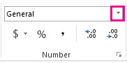
To distinguish between different types of numbers, add a format, like currency, percentages, or dates.
-
Select the cells that have numbers you want to format.
-
Click the Home tab, and then click the arrow in the General box.
-
Pick a number format.
If you don’t see the number format you’re looking for, click More Number Formats. For more information, see Available number formats.

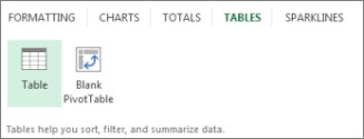
A simple way to access Excel’s power is to put your data in a table. That lets you quickly filter or sort your data.
-
Select your data by clicking the first cell and dragging to the last cell in your data.
To use the keyboard, hold down Shift while you press the arrow keys to select your data.
-
Click the Quick Analysis button
in the bottom-right corner of the selection.
-
Click Tables, move your cursor to the Table button to preview your data, and then click the Table button.
-
Click the arrow
in the table header of a column. -
To filter the data, clear the Select All check box, and then select the data you want to show in your table.
-
To sort the data, click Sort A to Z or Sort Z to A.
-
Click OK.
 in the bottom-right corner of the selection.
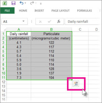
 in the table header of a column.
For more information, see Create or delete an Excel table
The Quick Analysis tool (available in Excel 2016 and Excel 2013 only) let you total your numbers quickly. Whether it’s a sum, average, or count you want, Excel shows the calculation results right below or next to your numbers.
-
Select the cells that contain numbers you want to add or count.
-
Click the Quick Analysis button
in the bottom-right corner of the selection. -
Click Totals, move your cursor across the buttons to see the calculation results for your data, and then click the button to apply the totals.
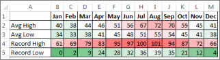
Conditional formatting or sparklines can highlight your most important data or show data trends. Use the Quick Analysis tool (available in Excel 2016 and Excel 2013 only) for a Live Preview to try it out.
-
Select the data you want to examine more closely.
-
Click the Quick Analysis button
in the bottom-right corner of the selection. -
Explore the options on the Formatting and Sparklines tabs to see how they affect your data.
For example, pick a color scale in the Formatting gallery to differentiate high, medium, and low temperatures.
-
When you like what you see, click that option.
 in the bottom-right corner of the selection.
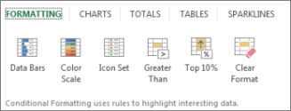
Learn more about how to analyze trends in data using sparklines.
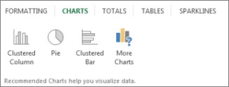
The Quick Analysis tool (available in Excel 2016 and Excel 2013 only) recommends the right chart for your data and gives you a visual presentation in just a few clicks.
-
Select the cells that contain the data you want to show in a chart.
-
Click the Quick Analysis button
in the bottom-right corner of the selection. -
Click the Charts tab, move across the recommended charts to see which one looks best for your data, and then click the one that you want.
Note: Excel shows different charts in this gallery, depending on what’s recommended for your data.
Learn about other ways to create a chart.
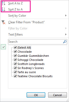
To quickly sort your data
-
Select a range of data, such as A1:L5 (multiple rows and columns) or C1:C80 (a single column). The range can include titles that you created to identify columns or rows.
-
Select a single cell in the column on which you want to sort.
-
Click
to perform an ascending sort (A to Z or smallest number to largest). -
Click
to perform a descending sort (Z to A or largest number to smallest).
 to perform an ascending sort (A to Z or smallest number to largest).
 to perform a descending sort (Z to A or largest number to smallest).
To sort by specific criteria
-
Select a single cell anywhere in the range that you want to sort.
-
On the Data tab, in the Sort & Filter group, choose Sort.
-
The Sort dialog box appears.
-
In the Sort by list, select the first column on which you want to sort.
-
In the Sort On list, select either Values, Cell Color, Font Color, or Cell Icon.
-
In the Order list, select the order that you want to apply to the sort operation — alphabetically or numerically ascending or descending (that is, A to Z or Z to A for text or lower to higher or higher to lower for numbers).
For more information about how to sort data, see Sort data in a range or table .
-
Select the data that you want to filter.
-
On the Data tab, in the Sort & Filter group, click Filter.
-
Click the arrow
in the column header to display a list in which you can make filter choices. -
To select by values, in the list, clear the (Select All) check box. This removes the check marks from all the check boxes. Then, select only the values you want to see, and click OK to see the results.
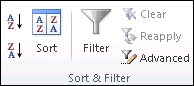
For more information about how to filter data, see Filter data in a range or table.
-
Click the Save button on the Quick Access Toolbar, or press Ctrl+S.
If you’ve saved your work before, you’re done.
-
If this is the first time you’ve save this file:
-
Under Save As, pick where to save your workbook, and then browse to a folder.
-
In the File name box, enter a name for your workbook.
-
Click Save.
-

-
Click File, and then click Print, or press Ctrl+P.
-
Preview the pages by clicking the Next Page and Previous Page arrows.
The preview window displays the pages in black and white or in color, depending on your printer settings.
If you don’t like how your pages will be printed, you can change page margins or add page breaks.
-
Click Print.

-
On the File tab, choose Options, and then choose the Add-Ins category.
-
Near the bottom of the Excel Options dialog box, make sure that Excel Add-ins is selected in the Manage box, and then click Go.
-
In the Add-Ins dialog box, select the check boxes the add-ins that you want to use, and then click OK.
If Excel displays a message that states it can’t run this add-in and prompts you to install it, click Yes to install the add-ins.
For more information about how to use add-ins, see Add or remove add-ins.
Excel allows you to apply built-in templates, to apply your own custom templates, and to search from a variety of templates on Office.com. Office.com provides a wide selection of popular Excel templates, including budgets.
For more information about how to find and apply templates, see Download free, pre-built templates.
Need more help?
Want more options?
Explore subscription benefits, browse training courses, learn how to secure your device, and more.
Communities help you ask and answer questions, give feedback, and hear from experts with rich knowledge.
Basic Excel Skills
Now a days, any job requires basic Excel skills. These basic Excel skills are – familiarity with Excel ribbons & UI, ability to enter and format data, calculate totals & summaries thru formulas, highlight data that meets certain conditions, creating simple reports & charts, understanding the importance of keyboard shortcuts & productivity tricks. Based on my experience of training more than 5,000 students in various online & physical training programs, the following 6 areas form the core of basic Excel skills.
Getting Started
Excel is a massive application with 1000s of features and 100s of ribbon (menu) commands. It is very easy to get lost once you open Excel. So one of the basic survival skills is to understand how to navigate Excel and access the features you are looking for.
When you open Excel, this is how it looks.

There are 5 important areas in the screen.
1. Quick Access Toolbar: This is a place where all the important tools can be placed. When you start Excel for the very first time, it has only 3 icons (Save, Undo, Redo). But you can add any feature of Excel to to Quick Access Toolbar so that you can easily access it from anywhere (hence the name).
2. Ribbon: Ribbon is like an expanded menu. It depicts all the features of Excel in easy to understand form. Since Excel has 1000s of features, they are grouped in to several ribbons. The most important ribbons are – Home, Insert, Formulas, Page Layout & Data.
3. Formula Bar: This is where any calculations or formulas you write will appear. You will understand the relevance of it once you start building formulas.
4. Spreadsheet Grid: This is where all your numbers, data, charts & drawings will go. Each Excel file can contain several sheets. But the spreadsheet grid shows few rows & columns of active spreadsheet. To see more rows or columns you can use the scroll bars to the left or at bottom. If you want to access other sheets, just click on the sheet name (or use the shortcut CTRL+Page Up or CTRL+Page Down).
5. Status bar: This tells us what is going on with Excel at any time. You can tell if Excel is busy calculating a formula, creating a pivot report or recording a macro by just looking at the status bar. The status bar also shows quick summaries of selected cells (count, sum, average, minimum or maximum values). You can change this by right clicking on it and choosing which summaries to show.
Getting Started with Excel – 10 minute video tutorial
Entering & Formatting Data, Numbers & Tables
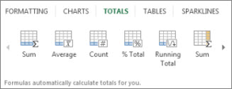
Calculating Totals & Summaries using Formulas
Conditional Formatting
Conditional formatting is a powerful feature in Excel that is often underutilized. By using conditional formatting, you can tell Excel to highlight portions of your data that meet any given condition. For example: highlighting top 10 customers, below average performing employees etc. While anyone can set up simple conditional formatting rules, an advanced Excel user can do a lot more. They can combine formulas with conditional formatting to highlight data that meets almost any condition.
Resources to learn Advanced Conditional Formatting
What is conditional formatting
Introduction to Conditional Formatting
5 Tips on CF
Highlighting Duplicates
More
Creating Reports Quickly
Using Excel Productively
Beyond Basics – Becoming Awesome in Excel
Once you know the basics, chances are you will be asking for more. The reason is simple. Anyone with good Excel skills is always in demand. Your bosses love you because you can get things done easily. Your customers love you becuase you create impressive things. Your colleagues envy you becuase your workbooks are shining and easy to use. And you want more, because you have seen the amazing results of Excel.
This is where learning Excel pays off. I highly recommend you to join my most comprehensive Excel training program – Excel School. It is an entirely online course that can be done at your own pace from the comfort of your home (or office). The course has more than 24 hours of training videos, 50+ downloadable workbooks, in-depth coverage of all the important areas of Excel usage to make you awesome. To date, more than 5,000 people have enrolled in Excel School and became champions at their work.
Click here to learn more about Excel School Program.
Explore the 20 most popular pages in this section. Below you can find a description of each page. Happy learning!
1 Drop-down List: Drop-down lists in Excel are helpful if you want to be sure that users select an item from a list, instead of typing their own values.
2 Lock Cells: You can lock cells in Excel if you want to protect cells from being edited.
3 Budget: This example shows you how to create a budget in Excel.
4 Checkbox: Inserting a checkbox in Excel is easy. For example, use checkboxes to create a checklist or a dynamic chart.
5 Time Sheet: This example teaches you how to create a simple timesheet calculator in Excel.
6 Freeze Panes: If you have a large table of data in Excel, it can be useful to freeze rows or columns. This way you can keep rows or columns visible while scrolling through the rest of the worksheet.
7 Delete Blank Rows: This example teaches you how to delete blank rows or rows that contain blank cells.
8 Merge Cells: Merge cells into one large cell to make clear that a label in Excel applies to multiple columns. Use CONCATENATE, TEXTJOIN or Flash Fill to merge cells without losing data.
9 Wrap Text: Wrap text in Excel if you want to display long text on multiple lines in a single cell.
10 Bullet Points: This page illustrates three ways to insert bullet points in Excel.
11 Check Mark: To insert a check mark symbol in Excel, simply press SHIFT + P and use the Wingdings 2 font.
12 Strikethrough: This example teaches you how to apply strikethrough formatting in Excel.
13 Show Formulas: By default, Excel shows the results of formulas. To show the formulas instead of their results, press CTRL + ` (you can find this key above the tab key).
14 Read-only Workbook: This example shows you how to make your Excel workbook read-only.
15 Superscript and Subscript: It’s easy to format a character as superscript (slightly above the baseline) or subscript (slightly below the baseline) in Excel.
16 Insert Row: To quickly insert a row in Excel, select a row and use the shortcut CTRL SHIFT +.
17 AutoRecover: Excel periodically saves a copy of your Excel file. Learn how to recover a file that was never saved and how to recover a file that has been saved at least once.
18 PDF: This page teaches you how to convert an Excel file to a PDF file.
19 Page Breaks: Insert a page break in Excel to specify where a new page will begin in the printed copy.
20 Calendar: This example describes how to create a calendar in Excel (2023 calendar, 2024 calendar, etc).
Check out all 300 examples.
Excel Basics Tutorials
Excel Basics tutorials are for beginners with no knowledge of Excel, in this section we cover the introduction to MS Excel, Objects and Tools available in Excel, Data entry and Formatting. By end of this session you will have understanding about Excel and be more confident using Excel to start work with excel.
Topics
In this section I will introduce the basic features of Microsoft Excel, one of the tools in the MS Office Package.
» Introduction to Microsoft Excel and Creating First Excel File:
Microsoft Excel is one of the tools in the Microsoft Office Package; it is used to create spreadsheets. It has many in-built functions and tools to work with data and create different type of reports and dashboards. It also provided the feature to the users to work behind the existing tools and can enhance its capabilities. To implement functionality beyond a regular spreadsheet, Microsoft Visual Basic programming environment is provided with Microsoft Office Excel. This programming language is called as Visual Basic for Application (VBA).
» Introduction to Excel Interface and Objects:
We have seen what is Excel and what we can achieve using Excel in the previous section. In this section we will what are the different objects in Excel to do our jobs and pictorial representation of Excel Interface.
» Entering Data and Moving in the Worksheet:
Entering Data and Moving in Excel Worksheet is very easy and you find that it is the time saver for data entry. You can enter any numbers, text, dates in Excel and you can format as per your requirement.
» Formatting Data and Formatting Cells:
One of the beauty of the Excel is rich formats, we can format the numbers, fonts, font color, background color, alignments and many more things we can do in Excel. This tutorial will help you to learn Formatting Data and Formatting Cells in Excel.
» Copying, Moving and Pasting Data:
When we are working with the data most of the time we may required to copy/move the data from one location (range) to another location. This tutorials will explains you Copying Moving and Pasting Data in Excel.
Downloads and Links
Downloads
» Excel Downloads
Useful Link
» Shortcut Keys
» Excel Tips
A Powerful & Multi-purpose Templates for project management. Now seamlessly manage your projects, tasks, meetings, presentations, teams, customers, stakeholders and time. This page describes all the amazing new features and options that come with our premium templates.
Save Up to 85% LIMITED TIME OFFER

All-in-One Pack
120+ Project Management Templates
Essential Pack
50+ Project Management Templates
Excel Pack
50+ Excel PM Templates
PowerPoint Pack
50+ Excel PM Templates
MS Word Pack
25+ Word PM Templates
Ultimate Project Management Template
Ultimate Resource Management Template
Project Portfolio Management Templates
Related Posts
VBA Reference
Effortlessly
Manage Your Projects
120+ Project Management Templates
Seamlessly manage your projects with our powerful & multi-purpose templates for project management.
120+ PM Templates Includes:
Effectively Manage Your
Projects and Resources
ANALYSISTABS.COM provides free and premium project management tools, templates and dashboards for effectively managing the projects and analyzing the data.
We’re a crew of professionals expertise in Excel VBA, Business Analysis, Project Management. We’re Sharing our map to Project success with innovative tools, templates, tutorials and tips.
Project Management
Excel VBA
Download Free Excel 2007, 2010, 2013 Add-in for Creating Innovative Dashboards, Tools for Data Mining, Analysis, Visualization. Learn VBA for MS Excel, Word, PowerPoint, Access, Outlook to develop applications for retail, insurance, banking, finance, telecom, healthcare domains.
Page load link

3 Realtime VBA Projects
with Source Code!
Go to Top