
Excel for Microsoft 365 Excel for Microsoft 365 for Mac Excel for the web Excel 2021 Excel 2021 for Mac Excel 2019 Excel 2019 for Mac Excel 2016 Excel 2016 for Mac Excel 2013 Excel 2010 Excel 2007 Excel for Mac 2011 Excel Starter 2010 More…Less
This article describes the formula syntax and usage of the ABS function in Microsoft Excel.
Description
Returns the absolute value of a number. The absolute value of a number is the number without its sign.
Syntax
ABS(number)
The ABS function syntax has the following arguments:
-
Number Required. The real number of which you want the absolute value.
Example
Copy the table below, and paste into cell A1 in Excel. You may need to select any cells that contain formulas and press F2 and then Enter to make the formulas work. You may also want to make the columns wider to make your worksheet easier to read.
|
Data |
||
|
-4 |
||
|
Formula |
Description |
Result |
|
=ABS(2) |
Absolute value of 2 |
2 |
|
=ABS(-2) |
Absolute value of -2 |
2 |
|
=ABS(A2) |
Absolute value of -4 |
4 |
See Also
Subtract numbers
Multiply and divide numbers in Excel
Calculate percentages
Need more help?
Want more options?
Explore subscription benefits, browse training courses, learn how to secure your device, and more.
Communities help you ask and answer questions, give feedback, and hear from experts with rich knowledge.
The ABS function in Excel returns the absolute value of a number. In other words: the ABS function removes the minus sign (-) from a negative number, making it positive.
1. For example, the ABS function in cell B1 below returns the absolute value of a negative number.

The ABS function has no effect on 0 (zero) or positive numbers.
2. The absolute value of 0 is 0.

3. The absolute value of a positive number is the same positive number.

When do we need the ABS function in Excel?
4. For example, calculate the forecast error (difference between the actual and the forecast value) for each month.

Note: if we look at the sum of these errors (zero), this forecast model seems perfect, but it’s not!
5. Simply use the ABS function to calculate the absolute error for each month.

6. If you don’t want to display the forecast errors on the sheet, use SUMPRODUCT and ABS.

Note: visit our page about the SUMPRODUCT function to learn more about this function.
Let’s take a look at one more cool example.
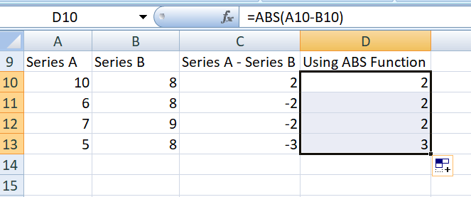
7. Use the ABS function to calculate the absolute value of each difference.

8. Add the IF function to test if the values are within tolerance.

Explanation: if the difference is less than or equal to 3, the IF function returns 1, else it returns 0.
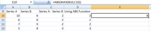
9. Add icons.
![]()
10. Change the tolerance.

Note: visit our page about icon sets to learn more about this topic. To view this formatting rule, download the Excel file. Next, on the Home tab, in the Styles group, click Conditional Formatting, Manage Rules.
Returns the absolute value of a number
What is the ABSOLUTE Function in Excel (ABS)?
The ABS Function[1] in Excel returns the absolute value of a number. The function converts negative numbers to positive numbers while positive numbers remain unaffected.
Formula
ABSOLUTE Value = ABS(number)
Where number is the numeric value for which we need to calculate the Absolute value.
How to use the ABSOLUTE Function in Excel?
Let’s take a series of numbers to understand how this function can be used.
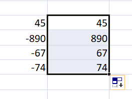
In the screenshot above, we are given a series of numbers. When we use the ABSOLUTE function, we get the following results:
- For positive numbers, we get the same result. So 45 is returned as 45.
- For negative numbers, the function returns absolute numbers. So for -890, -67, -74, we got 890, 67, 74.
To learn more, launch our free Excel crash course now!
Examples of the ABSOLUTE Function in Excel
For our analysis, we want the difference between Series A and Series B as given below. Ideally, if you subtract Series A from Series B you might get negative numbers depending on the values. However, if you want absolute numbers in this scenario, we can use the ABSOLUTE function.
The results returned using ABSOLUTE function would be absolute numbers. So ABS can be combined with other functions such as SUM, MAX, MIN, AVERAGE, etc. to calculate the absolute value for positive and negative numbers in Excel spreadsheets.
Let’s see a few examples of how ABS can be used with other Excel Functions.
1. SUMIF and ABS
We all are aware that SUMIF would sum up values if certain criteria within the range given are met. Let’s assume we’ve been given a few numbers in Column A and Column B as below:
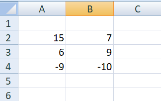
Now, I wish to subtract all negative numbers in Column B from all positive numbers of Column A. I want the result to be an absolute number. So I can use the ABS function along with SUMIF in the following manner:
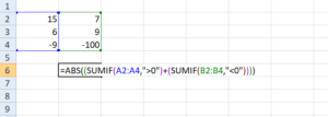
The result is 79. Excel added 15 and 6 from Column A and subtracted 100 from Column B to give us 79, as we used ABS function instead of -79.
2. SUM ARRAY Formula and ABS Function
The Excel array formulas help us to do multiple calculations for a given array or column of values. We can use SUM ARRAY along with ABS to get the absolute value of a series of numbers in column or row. Suppose we are given a few numbers as below, so in this scenario, the SUM array formula for absolute values would be =SUM(ABS(A2:A6)).
Now, select cell A7 in your spreadsheet, and enter the formula ‘=SUM(ABS(A2:A6))’. After entering the formula in cell A7, press “Ctrl + Shift + Enter”. Once we do this, the formula will have {} brackets around it as shown in the screenshot below.
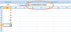
As seen in the screenshot above, the array formula also returned the value 44 in cell A7, which is the absolute value of the data entered in cells A2:A6.
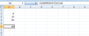
3. SUMPRODUCT Formula and ABS Function
The SUMPRODUCT function allows us to include the ABS function to provide absolute numbers. Suppose we are given the following data. If we would just use the SUMPRODUCT formula, we would get a negative number as shown below:
However, using ABS Function, we can get the absolute number as a result. The formula to be used would be:
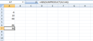
To learn more, launch our free Excel crash course now!
ABS as a VBA Function
If we wish to use the ABSOLUTE function in Excel VBA code, it can be used in the following manner. Let’s assume I need ABS of -600 so the code would be:
Dim LNumber As Double
LNumber = ABS(-600)
Now in the above code, the variable known as LNumber would now contain the value of 600.
Free Excel Course
If you want to learn more Excel functions with your own online instructor, check out CFI’s Free Excel Crash Course! You’ll get step by step tutorials and demonstrations on how to become an Excel power user.
Additional Resources
Thanks for reading CFI’s guide to important Excel functions! By taking the time to learn and master these functions, you’ll significantly speed up your financial analysis. To learn more, check out these additional CFI resources:
- Excel Functions for Finance
- Advanced Excel Formulas Course
- Advanced Excel Formulas You Must Know
- Excel Shortcuts for PC and Mac
- See all Excel resources
Article Sources
- ABS Function
Purpose
Find the absolute value of a number
Usage notes
The ABS function returns the absolute value of a number. You can think about absolute value as a number’s distance from zero on a number line. ABS converts negative numbers to positive numbers. Positive numbers and zero (0) are unaffected.
The ABS function takes just one argument, number, which must be a numeric value. If number is not numeric, ABS returns a #VALUE! error.
Basic example
Negative numbers become positive, while positive numbers and zero (0) are unaffected:
=ABS(-3) // returns 3
=ABS(5) // returns 5
=ABS(0) // returns 0
Absolute Variance
Calculating the variance between two numbers is a common problem. For example, with a forecast value in A1 and an actual value in B1, you might calculate variance like this:
=B1-A1 // negative or positive result
When B1 is greater than A1, variance is a positive number. However, when A1 is greater than B1, the result will be negative. To ensure the result is a positive number, you can use ABS like this:
=ABS(B1-A1) // ensure positive result
See a detailed example here.
Counting absolute variances with conditions
The ABS function can be used together with the SUMPRODUCT function to count absolute variances that meet specific conditions. For example, to count absolute variances greater than 100, you can use a formula like this:
=SUMPRODUCT(--(ABS(variances)>100))
This formula is explained in more detail here.
Square root of negative number
The SQRT function calculates the square root of a number. If you give SQRT a negative number, it will return a #NUM! error:
=SQRT(-4) // returns #NUM!
To handle a negative number like a positive number, you can use the ABS function like this:
=SQRT(ABS(A1))
Calculating tolerance
To calculate whether a value is within tolerance or not, you can use a formula like this:
=IF(ABS(actual-expected)<=tolerance,"OK","Fail")
See a detailed explanation here.
Excel Absolute Value (Table of Contents)
- Absolute Value in Excel
- Methods of Absolute Functions in Excel
- How to Use Absolute value in excel?
Absolute Value in Excel
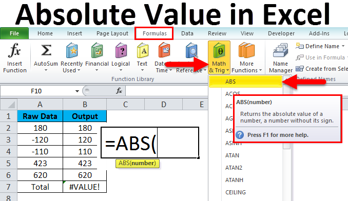
Absolute Value in Excel can be calculated using the ABS function, which is available under the category of Math and Trig in Insert function. Absolute Value is the positive form of any negative value whether is it an integer number or decimal number. To use the ABS function, go to the Insert function option from the Formula menu tab in Excel and select ABS function, or else we can directly select ABS function by going in the edit mode of any cell. Then select those cells that contain negative values as per syntax. We will see, it would get converted into positive absolute value.
Absolute Formula in Excel
Below is the Absolute Formula in Excel :
The Absolute Value Formula in excel has one argument:
- Number – which is used to get the absolute value of the number.
Methods of Absolute Functions in Excel
In Microsoft excel, the ABS function comes under the category of Math and Trigonometric, where we can find the Math and Trigonometric in the Formula menu; we will see how to use the ABS function by following the below steps.
- First, go to the Formulas option.
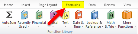
- In the formula menu, we can see the Math & Trig option.
- Click on the Math & Trig option so that we will get the list of functions which is shown in the below screenshot.
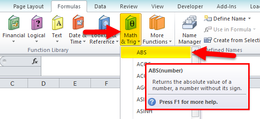
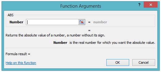
- Click on the first function called ABS.
- We will get the ABS function dialogue box as shown below.
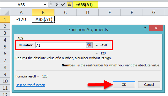
- Select the negative number on the cell as shown in the below screenshot.
- Click OK
- The given negative number will be returned as an absolute positive number.
How to Use Absolute value in excel?
Absolute Value in Excel is very simple and easy to use. Let’s understand the working of excel Absolute Value with some examples.
You can download this Absolute Value Excel Template here – Absolute Value Excel Template
Excel Absolute Value – Example #1
In this example, we are going to see how to use the ABS function by following the below steps.
Consider the below example, which has some random positive and negative numbers.
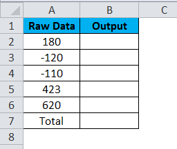
Now we are going to use the ABS function, which will return the positive number by following the below procedure.
- Click on the Output column.
- Use ABS formula as =ABS(A2) as shown in the below screenshot.
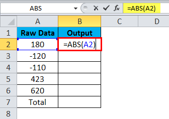
- Press ENTER; we will get the output as follows.
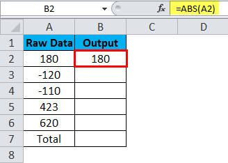
- In the above screenshot, the first row contains a positive number, so there is no difference, and the ABS function returned the absolute value of the number.
- Drag down the formula for all the cell
- We will get the below output as follows.

- As we can see that in the second row, we have a negative number; by using the ABS function, we have converted a negative number to a positive number, and the positive number remains unchanged.
- At last, we can see the VALUE error because the ABS function will throw a VALUE error If the supplied argument is non-numeric.
Excel Absolute Value – Example #2
Using Addition in ABS function
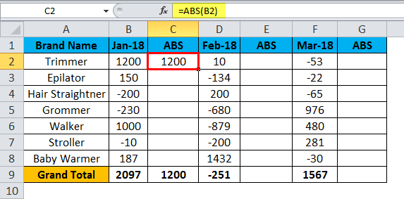
In this example, we are going to see how the ABS function work using SUM. Consider the below example, which has product wise sales figure for three months.
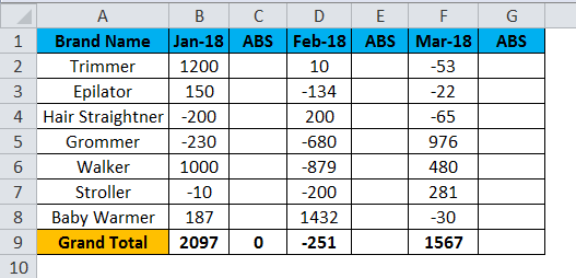
In the above screenshot, we can see that the grand total has been calculated using the SUM formula.
Let us use the ABS function and check for the final grand value by following the below steps.
- First, click on cell C2.
- Insert the ABS function formula as =ABS(B2) shown below.
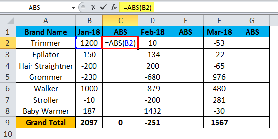
- Click ENTER.
- The absolute function checks for the number, and it will return the absolute number.
- We will get the output as follows, as shown in the below screenshot.
- Drag down the formula for all the cells so that we will get the final out output as follows.
- As we can see in the above screenshot, the ABS function returned the absolute number and converted the negative number to positive numbers.
- We can notice that the grand total value has a huge difference after using the ABS function because SUM will add the positive numbers and subtract the negative numbers and give the end result.
- Here ABS function converted all negative numbers to positive numbers, and we got the grand total with a positive number.
- Do the same operation and apply the ABS function to the E and H column, and we will get the below result as follows.
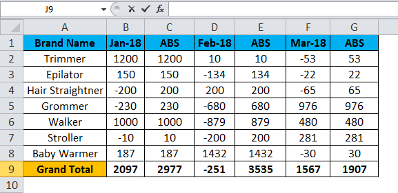
In the above result, we can see the Grand total difference after applying the ABS function.
Excel Absolute Value – Example#3
Using Subtraction in ABS function
In this example, we are going to see how the ABS function works in subtraction. Let’s consider the below example, which shows the month-wise sales data of each employee and the difference.
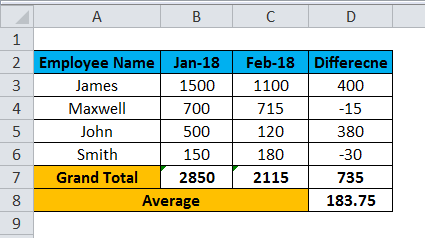
We can notice that we got the difference minus sign figure for the salesperson MAXWELL and the salesperson SMITH in the above screenshot. We have used the subtraction formula as Jan sales value – Feb sales value as shown in the below screenshot.
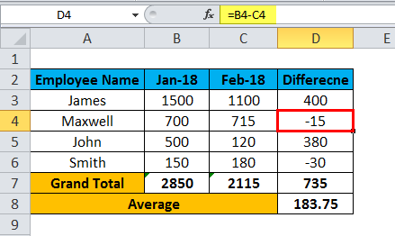
Here we have used the formulation as =B4-C4 as we cannot subtract lower value with higher value, and while doing sales analysis, this report will go wrong because of the negative figure and also we can see that Average also seems to be wrong due to the negative figure. In order to overcome these errors, we can use the ABS function by following the below steps.
- Click on the D column cell named Difference.
- Use the ABS function as =ABS (B3-C3) will check for the number and return the absolute value shown in the below screenshot.
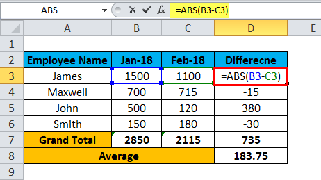
- Click ENTER, and we will get the output as shown below.
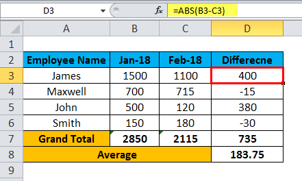
- Drag down the formula for all the cells so that we will get the final output as shown.
- This is the correct way of reporting that the ABS function converted the negative number to a positive number, which gives the exact report.
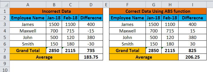
In the above comparison result, we can see the difference that before applying the ABS function, we got some different figures which is actually an incorrect way of doing subtraction.
We can notice that after applying the ABS function, it returned the absolute value, and we can see the changed in Grand total where it was 735 before and after applying the ABS function, we got the Grand total as 825.
We can notice the same difference in Average where it was 183.7 before and after applying the ABS function; we got an average of 206.25, which is the exact average of the sales report.
Things to Remember
- ABS function in excel normally returns the absolute values. Which converts negative numbers to positive numbers
- While using the ABS function, we can see that positive numbers are unaffected.
- ABS function in excel will throw a #VALUE! error if the supplied argument is non-numeric.
- While using the ABS function, make sure that all arguments are numeric values.
Recommended Articles
This has been a guide to Absolute Value in Excel. Here we discuss how to use the Absolute Value in Excel along with practical examples and a downloadable excel template. You can also go through our other suggested articles –
- ABS Function in Excel
- Excel Absolute Reference
- Relative Reference in Excel
- Statistics in Excel