
Содержание
- Применение абсолютной адресации
- Способ 1: абсолютная ссылка
- Способ 2: функция ДВССЫЛ
- Вопросы и ответы

Как известно, в таблицах Excel существует два вида адресации: относительная и абсолютная. В первом случае ссылка изменяется по направлению копирования на относительную величину сдвига, а во втором — является фиксированной и при копировании остается неизменной. Но по умолчанию все адреса в Экселе являются абсолютными. В то же время, довольно часто присутствует необходимость использовать абсолютную (фиксированную) адресацию. Давайте узнаем, какими способами это можно осуществить.
Применение абсолютной адресации
Абсолютная адресация нам может понадобиться, например, в том случае, когда мы копируем формулу, одна часть которой состоит из переменной, отображаемой в ряду чисел, а вторая имеет постоянное значение. То есть, данное число играет роль неизменного коэффициента, с которым нужно провести определенную операцию (умножение, деление и т.д.) всему ряду переменных чисел.
В Excel существует два способа задать фиксированную адресацию: путем формирования абсолютной ссылки и с помощью функции ДВССЫЛ. Давайте рассмотрим каждый из указанных способов подробно.
Способ 1: абсолютная ссылка
Безусловно, самым известным и часто применяемым способом создать абсолютную адресацию является применение абсолютных ссылок. Абсолютные ссылки имеют отличие не только функциональное, но и синтаксическое. Относительный адрес имеет такой синтаксис:
=A1
У фиксированного адреса перед значением координат устанавливается знак доллара:
=$A$1

Знак доллара можно ввести вручную. Для этого нужно установить курсор перед первым значением координат адреса (по горизонтали), находящегося в ячейке или в строке формул. Далее, в англоязычной раскладке клавиатуры следует кликнуть по клавише «4» в верхнем регистре (с зажатой клавишей «Shift»). Именно там расположен символ доллара. Затем нужно ту же процедуру проделать и с координатами по вертикали.
Существует и более быстрый способ. Нужно установить курсор в ячейку, в которой находится адрес, и щелкнуть по функциональной клавише F4. После этого знак доллара моментально появится одновременно перед координатами по горизонтали и вертикали данного адреса.
Теперь давайте рассмотрим, как применяется на практике абсолютная адресация путем использования абсолютных ссылок.
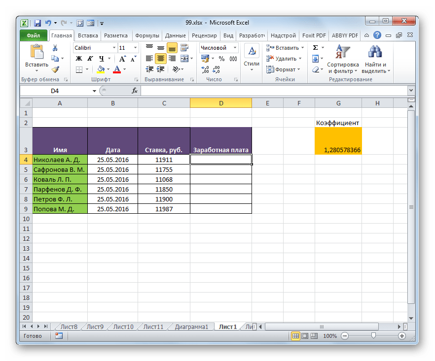
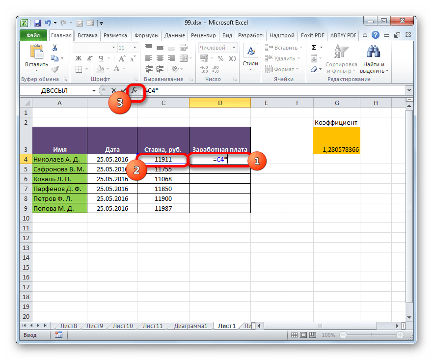
Возьмем таблицу, в которой рассчитывается заработная плата работников. Расчет производится путем умножения величины их личного оклада на фиксированный коэффициент, который одинаков для всех сотрудников. Сам коэффициент расположен в отдельной ячейке листа. Перед нами стоит задача рассчитать заработную плату всех работников максимально быстрым способом.
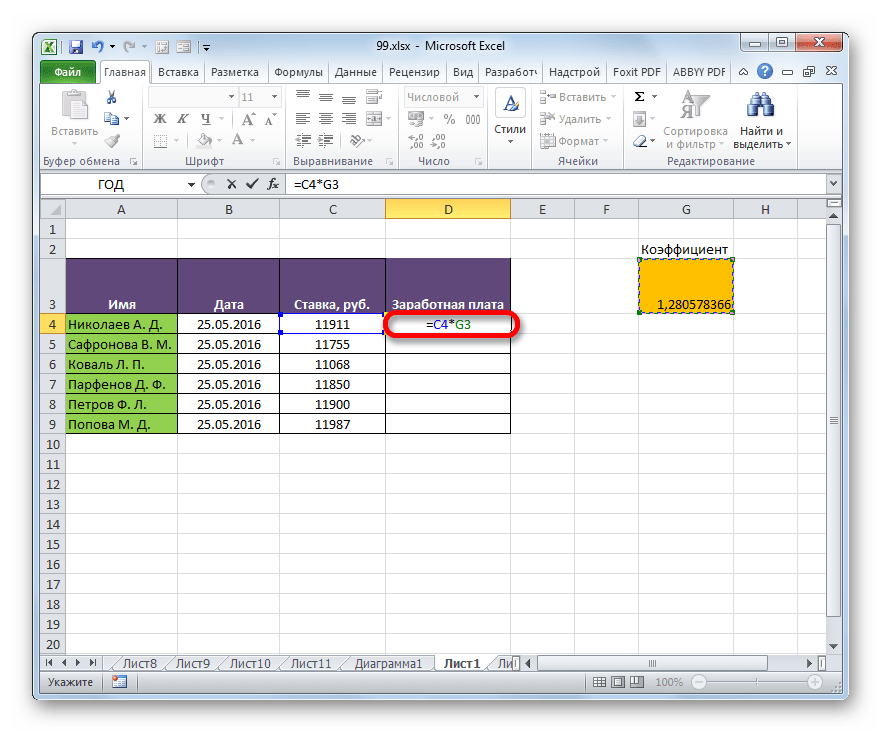
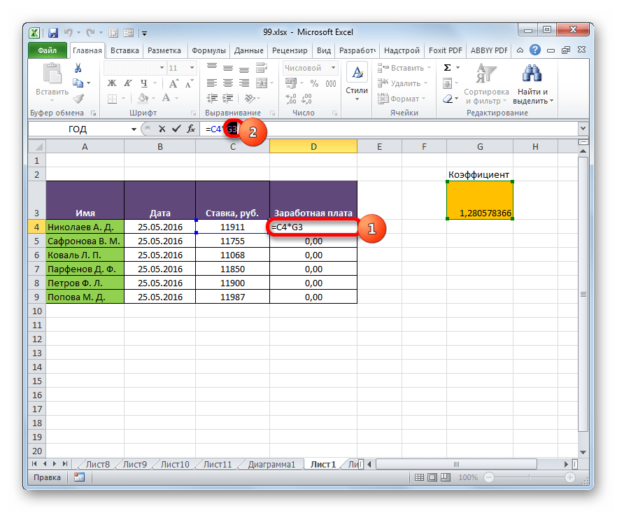
- Итак, в первую ячейку столбца «Заработная плата» вводим формулу умножения ставки соответствующего работника на коэффициент. В нашем случае эта формула имеет такой вид:
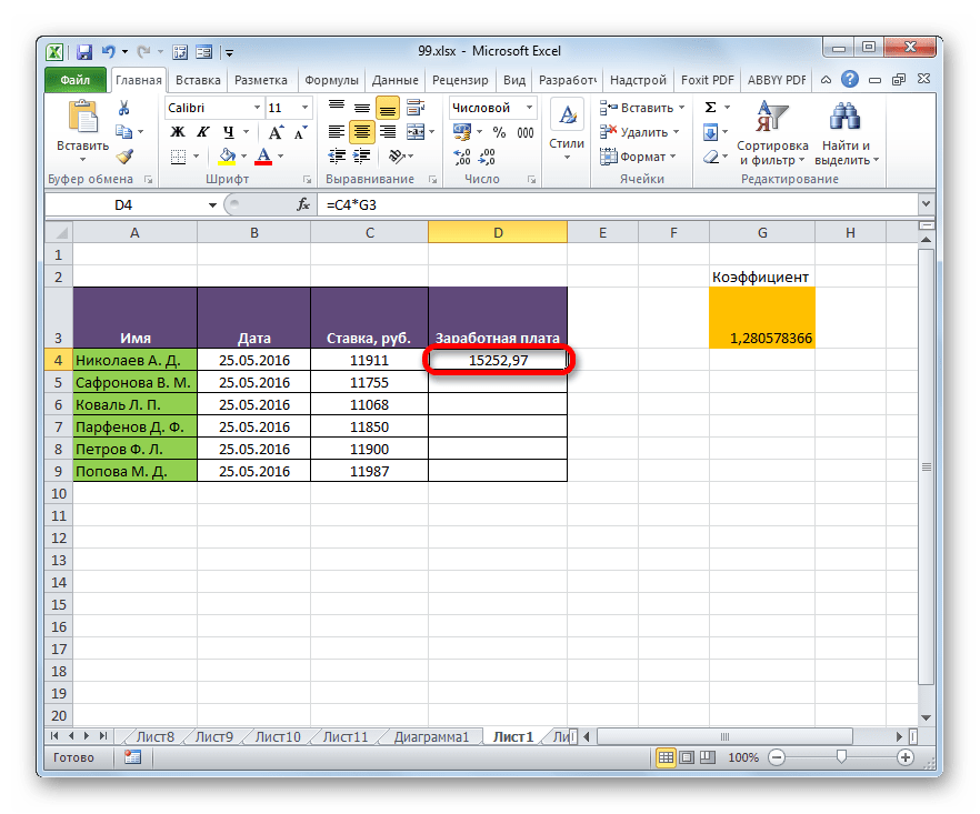
=C4*G3 - Чтобы рассчитать готовый результат, щелкаем по клавише Enter на клавиатуре. Итог выводится в ячейку, содержащую формулу.
- Мы рассчитали значение зарплаты для первого сотрудника. Теперь нам нужно это сделать для всех остальных строк. Конечно, операцию можно записать в каждую ячейку столбца «Заработная плата» вручную, вводя аналогичную формулу с поправкой на смещение, но у нас стоит задача, как можно быстрее выполнить вычисления, а ручной ввод займет большое количество времени. Да и зачем тратить усилия на ручной ввод, если формулу можно попросту скопировать в другие ячейки?
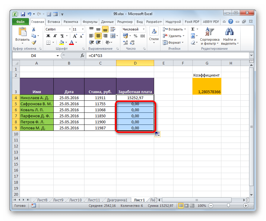
Для копирования формулы применим такой инструмент, как маркер заполнения. Становимся курсором в нижний правый угол ячейки, где она содержится. При этом сам курсор должен преобразоваться в этот самый маркер заполнения в виде крестика. Зажимаем левую кнопку мыши и тянем курсор вниз до конца таблицы.
- Но, как видим, вместо корректного расчета заработной платы для остальных сотрудников, мы получили одни нули.
- Смотрим, в чем причина такого результата. Для этого выделяем вторую ячейку в столбце «Заработная плата». В строке формул отображается соответствующее данной ячейке выражение. Как видим, первый множитель (C5) соответствует ставке того работника, зарплату которого мы рассчитываем. Смещение координат по сравнению с предыдущей ячейкой произошло из-за свойства относительности. Впрочем, в конкретно данном случае это нам и нужно. Благодаря этому первым множителем стала ставка именно нужного нам работника. Но смещение координат произошло и со вторым множителем. И теперь его адрес ссылается не на коэффициент (1,28), а на пустую ячейку, расположенную ниже.

Именно это и послужило причиной того, что расчет заработной платы для последующих сотрудников из списка получился некорректным.
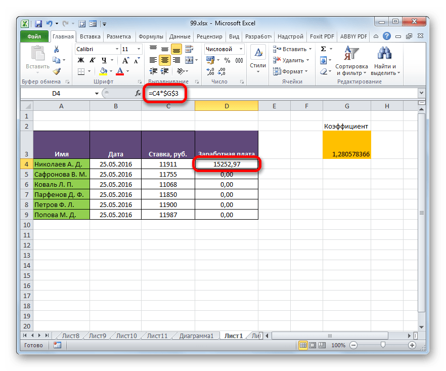
- Для исправления ситуации нам нужно изменить адресацию второго множителя с относительной на фиксированную. Для этого возвращаемся к первой ячейке столбца «Заработная плата», выделив её. Далее перемещаемся в строку формул, где отобразилось нужное нам выражение. Выделяем курсором второй множитель (G3) и жмем на функциональную клавишу на клавиатуре.
- Как видим, около координат второго множителя появился знак доллара, а это, как мы помним, является атрибутом абсолютной адресации. Чтобы вывести результат на экран жмем на клавишу Enter.
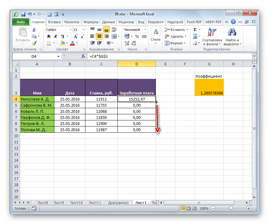
- Теперь, как и ранее вызываем маркер заполнения, установив курсор в правый нижний угол первого элемента столбца «Заработная плата». Зажимаем левую кнопку мыши и тянем его вниз.
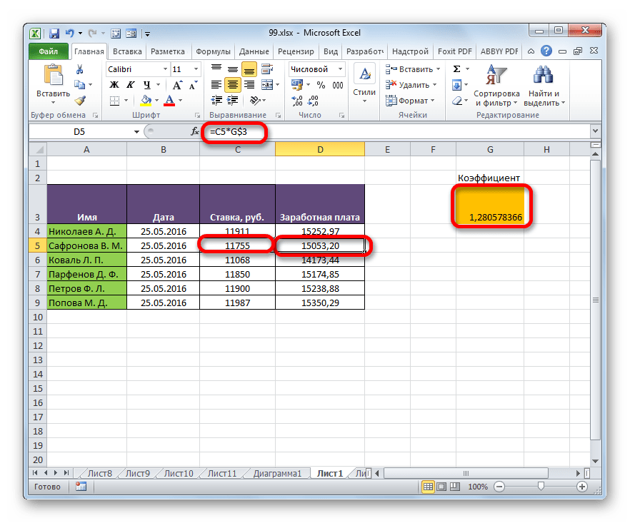
- Как видим, в данном случае расчет был проведен верно и сумма заработной платы для всех работников предприятия рассчитана корректно.
- Проверим, как была скопирована формула. Для этого выделяем второй элемент столбца «Заработная плата». Смотрим на выражение, расположенное в строке формул. Как видим, координаты первого множителя (C5), который по прежнему является относительным, сдвинулись по сравнению с предыдущей ячейкой на один пункт вниз по вертикали. Зато второй множитель ($G$3), адресацию в котором мы сделали фиксированной, остался неизменным.


В Экселе также применяется, так называемая смешанная адресация. В этом случае в адресе элемента фиксируется либо столбец, либо строка. Достигается это таким образом, что знак доллара ставится только перед одним из координат адреса. Вот пример типичной смешанной ссылки:
=A$1

Этот адрес тоже считается смешанным:
=$A1

То есть, абсолютная адресация в смешанной ссылке используется только для одного из значений координат из двух.
Посмотрим, как такую смешанную ссылку можно применить на практике на примере все той же таблицы заработной платы сотрудников предприятия.
- Как видим, ранее мы сделали так, что все координаты второго множителя имеют абсолютную адресацию. Но давайте разберемся, обязательно ли в этом случае оба значения должны быть фиксированными? Как видим, при копировании происходит смещение по вертикали, а по горизонтали координаты остаются неизменными. Поэтому вполне можно применить абсолютную адресацию только к координатам строки, а координаты столбца оставить такими, каковыми они являются по умолчанию – относительными.
Выделяем первый элемент столбца «Заработная плата» и в строке формул выполняем вышеуказанную манипуляцию. Получаем формулу следующего вида:
=C4*G$3Как видим, фиксированная адресация во втором множителе применяется только по отношению к координатам строки. Для вывода результата в ячейку щелкаем по кнопке Enter.
- После этого посредством маркера заполнения копируем данную формулу на диапазон ячеек, который расположен ниже. Как видим, расчет заработной платы по всем сотрудникам выполнен корректно.
- Смотрим, как отображается скопированная формула во второй ячейке столбца, над которым мы выполняли манипуляцию. Как можно наблюдать в строке формул, после выделения данного элемента листа, несмотря на то, что абсолютную адресацию у второго множителя имели только координаты строк, смещение координат столбца не произошло. Это связано с тем, что мы выполняли копирование не по горизонтали, а по вертикали. Если бы мы выполнили копирование по горизонтали, то в аналогичном случае, наоборот, пришлось бы делать фиксированную адресацию координат столбцов, а для строк эта процедура была бы необязательной.


Урок: Абсолютные и относительные ссылки в Экселе
Способ 2: функция ДВССЫЛ
Вторым способом организовать абсолютную адресацию в таблице Excel является применение оператора ДВССЫЛ. Указанная функция относится к группе встроенных операторов «Ссылки и массивы». Её задачей является формирование ссылки на указанную ячейку с выводом результата в тот элемент листа, в котором находится сам оператор. При этом ссылка прикрепляется к координатам ещё крепче, чем при использовании знака доллара. Поэтому иногда принято называть ссылки с использованием ДВССЫЛ «суперабсолютными». Этот оператор имеет следующий синтаксис:
=ДВССЫЛ(ссылка_на_ячейку;[a1])
Функция имеет в наличии два аргумента, первый из которых имеет обязательный статус, а второй – нет.
Аргумент «Ссылка на ячейку» является ссылкой на элемент листа Excel в текстовом виде. То есть, это обычная ссылка, но заключенная в кавычки. Именно это и позволяет обеспечить свойства абсолютной адресации.
Аргумент «a1» — необязательный и используется в редких случаях. Его применение необходимо только тогда, когда пользователь выбирает альтернативный вариант адресации, а не обычное использование координат по типу «A1» (столбцы имеют буквенное обозначение, а строки — цифровое). Альтернативный вариант подразумевает использование стиля «R1C1», в котором столбцы, как и строки, обозначаются цифрами. Переключиться в данный режим работы можно через окно параметров Excel. Тогда, применяя оператор ДВССЫЛ, в качестве аргумента «a1» следует указать значение «ЛОЖЬ». Если вы работает в обычном режиме отображения ссылок, как и большинство других пользователей, то в качестве аргумента «a1» можно указать значение «ИСТИНА». Впрочем, данное значение подразумевается по умолчанию, поэтому намного проще вообще в данном случае аргумент «a1» не указывать.
Взглянем, как будет работать абсолютная адресация, организованная при помощи функции ДВССЫЛ, на примере нашей таблицы заработной платы.
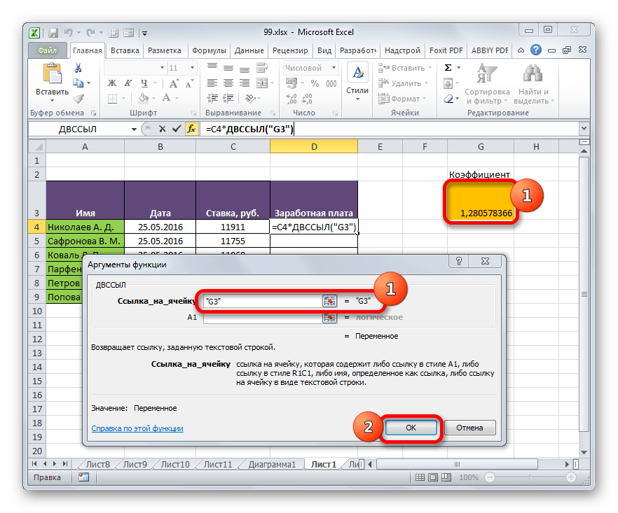
- Производим выделение первого элемента столбца «Заработная плата». Ставим знак «=». Как помним, первый множитель в указанной формуле вычисления зарплаты должен быть представлен относительным адресом. Поэтому просто кликаем на ячейку, содержащую соответствующее значение оклада (C4). Вслед за тем, как её адрес отобразился в элементе для вывода результата, жмем на кнопку «умножить» (*) на клавиатуре. Затем нам нужно перейти к использованию оператора ДВССЫЛ. Выполняем щелчок по иконке «Вставить функцию».
- В открывшемся окне Мастера функций переходим в категорию «Ссылки и массивы». Среди представленного списка названий выделяем наименование «ДВССЫЛ». Затем щелкаем по кнопке «OK».
- Производится активация окошка аргументов оператора ДВССЫЛ. Оно состоит из двух полей, которые соответствуют аргументам этой функции.
Ставим курсор в поле «Ссылка на ячейку». Просто кликаем по тому элементу листа, в котором находится коэффициент для расчета зарплаты (G3). Адрес тут же появится в поле окна аргументов. Если бы мы имели дело с обычной функцией, то на этом введение адреса можно было бы считать завершенным, но мы используем функцию ДВССЫЛ. Как мы помним, адреса в ней должны иметь вид текста. Поэтому оборачиваем координаты, которые расположись в поле окна, кавычками.
Так как мы работаем в стандартном режиме отображения координат, то поле «A1» оставляем незаполненным. Щелкаем по кнопке «OK».
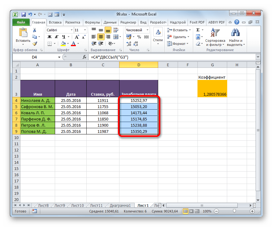
- Приложение выполняет вычисление и выводит результат в элемент листа, содержащий формулу.
- Теперь производим копирование данной формулы во все остальные ячейки столбца «Заработная плата» посредством маркера заполнения, как мы это делали ранее. Как видим, все результаты были рассчитаны верно.
- Посмотрим, как отображается формула в одной из ячеек, куда она была скопирована. Выделяем второй элемент столбца и смотрим на строку формул. Как видим, первый множитель, являющийся относительной ссылкой, изменил свои координаты. В то же время, аргумент второго множителя, который представлен функцией ДВССЫЛ, остался неизменным. В данном случае была использована методика фиксированной адресации.


Урок: Оператор ДВССЫЛ в Экселе
Абсолютную адресацию в таблицах Excel можно обеспечить двумя способами: использование функции ДВССЫЛ и применение абсолютных ссылок. При этом функция обеспечивает более жесткую привязку к адресу. Частично абсолютную адресацию можно также применять при использовании смешанных ссылок.
Excel for Microsoft 365 Excel for the web Excel 2021 Excel 2019 Excel 2016 Excel 2013 Excel Web App Excel 2010 Excel 2007 More…Less
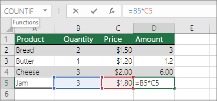
By default, a cell reference is a relative reference, which means that the reference is relative to the location of the cell. If, for example, you refer to cell A2 from cell C2, you are actually referring to a cell that is two columns to the left (C minus A)—in the same row (2). When you copy a formula that contains a relative cell reference, that reference in the formula will change.
As an example, if you copy the formula =B4*C4 from cell D4 to D5, the formula in D5 adjusts to the right by one column and becomes =B5*C5. If you want to maintain the original cell reference in this example when you copy it, you make the cell reference absolute by preceding the columns (B and C) and row (2) with a dollar sign ($). Then, when you copy the formula =$B$4*$C$4 from D4 to D5, the formula stays exactly the same.
Less often, you may want to mixed absolute and relative cell references by preceding either the column or the row value with a dollar sign—which fixes either the column or the row (for example, $B4 or C$4).
To change the type of cell reference:
-
Select the cell that contains the formula.
-
In the formula bar
 , select the reference that you want to change.
 -
Press F4 to switch between the reference types.
The table below summarizes how a reference type updates if a formula containing the reference is copied two cells down and two cells to the right.
 , select the reference that you want to change.
|
For a formula being copied: |
If the reference is: |
It changes to: |
|
|
$A$1 (absolute column and absolute row) |
$A$1 (the reference is absolute) |
|
A$1 (relative column and absolute row) |
C$1 (the reference is mixed) |
|
|
$A1 (absolute column and relative row) |
$A3 (the reference is mixed) |
|
|
A1 (relative column and relative row) |
C3 (the reference is relative) |
Need more help?
Преимущества абсолютных ссылок сложно недооценить. Их часто приходится использовать в процессе работы с программой. Относительные ссылки на ячейки в Excel более популярные чем, абсолютные, но так же имеют свои плюсы и минусы.
В Excel существует несколько типов ссылок: абсолютные, относительные и смешанные. Сюда так же относятся «имена» на целые диапазоны ячеек. Рассмотрим их возможности и отличия при практическом применении в формулах.
Абсолютные и относительные ссылки в Excel
Абсолютные ссылки позволяют нам зафиксировать строку или столбец (или строку и столбец одновременно), на которые должна ссылаться формула. Относительные ссылки в Excel изменяются автоматически при копировании формулы вдоль диапазона ячеек, как по вертикали, так и по горизонтали. Простой пример относительных адресов ячеек:
- Заполните диапазон ячеек A2:A5 разными показателями радиусов.
- В ячейку B2 введите формулу вычисления объема сферы, которая будет ссылаться на значение A2. Формула будет выглядеть следующим образом: =(4/3)*3,14*A2^3
- Скопируйте формулу из B2 вдоль колонки A2:A5.
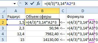
Как видите, относительные адреса помогают автоматически изменять адрес в каждой формуле.
Так же стоит отметить закономерность изменения ссылок в формулах. Данные в B3 ссылаются на A3, B4 на A4 и т.д. Все зависит од того куда будет ссылаться первая введенная формула, а ее копии будут изменять ссылки относительно своего положения в диапазоне ячеек на листе.
Использование абсолютных и относительных ссылок в Excel
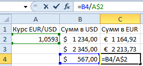
Заполните табличку, так как показано на рисунке:
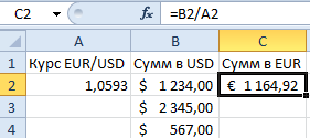
Описание исходной таблицы. В ячейке A2 находиться актуальный курс евро по отношению к доллару на сегодня. В диапазоне ячеек B2:B4 находятся суммы в долларах. В диапазоне C2:C4 будут находится суммы в евро после конвертации валют. Завтра курс измениться и задача таблички автоматически пересчитать диапазон C2:C4 в зависимости от изменения значения в ячейке A2 (то есть курса евро).
Для решения данной задачи нам нужно ввести формулу в C2: =B2/A2 и скопировать ее во все ячейки диапазона C2:C4. Но здесь возникает проблема. Из предыдущего примера мы знаем, что при копировании относительные ссылки автоматически меняют адреса относительно своего положения. Поэтому возникнет ошибка:
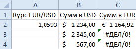
Относительно первого аргумента нас это вполне устраивает. Ведь формула автоматически ссылается на новое значение в столбце ячеек таблицы (суммы в долларах). А вот второй показатель нам нужно зафиксировать на адресе A2. Соответственно нужно менять в формуле относительную ссылку на абсолютную.
Как сделать абсолютную ссылку в Excel? Очень просто нужно поставить символ $ (доллар) перед номером строки или колонки. Или перед тем и тем. Ниже рассмотрим все 3 варианта и определим их отличия.
Наша новая формула должна содержать сразу 2 типа ссылок: абсолютные и относительные.
- В C2 введите уже другую формулу: =B2/A$2. Чтобы изменить ссылки в Excel сделайте двойной щелчок левой кнопкой мышки по ячейке или нажмите клавишу F2 на клавиатуре.
- Скопируйте ее в остальные ячейки диапазона C3:C4.
Описание новой формулы. Символ доллара ($) в адресе ссылок фиксирует адрес в новых скопированных формулах.
Абсолютные, относительные и смешанные ссылки в Excel:
- $A$2 – адрес абсолютной ссылки с фиксацией по колонкам и строкам, как по вертикали, так и по горизонтали.
- $A2 – смешанная ссылка. При копировании фиксируется колонка, а строка изменяется.
- A$2 – смешанная ссылка. При копировании фиксируется строка, а колонка изменяется.
Для сравнения: A2 – это адрес относительный, без фиксации. Во время копирования формул строка (2) и столбец (A) автоматически изменяются на новые адреса относительно расположения скопированной формулы, как по вертикали, так и по горизонтали.
Примечание. В данном примере формула может содержать не только смешанную ссылку, но и абсолютную: =B2/$A$2 результат будет одинаковый. Но в практике часто возникают случаи, когда без смешанных ссылок не обойтись.
Полезный совет. Чтобы не вводить символ доллара ($) вручную, после указания адреса периодически нажимайте клавишу F4 для выбора нужного типа: абсолютный или смешанный. Это быстро и удобно.
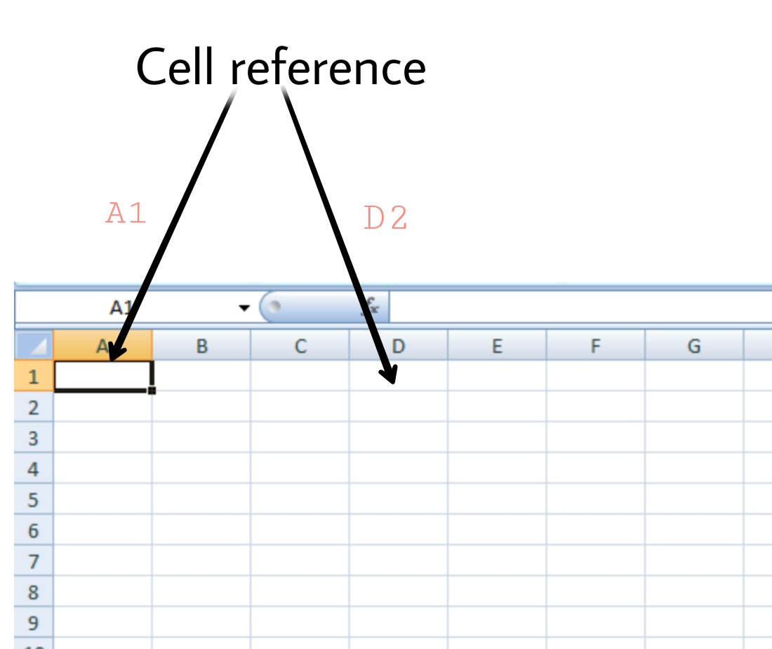
Cell reference is the address or name of a cell or a range of cells. It is the combination of column name and row number. It helps the software to identify the cell from where the data/value is to be used in the formula. We can reference the cell of other worksheets and also of other programs.
- Referencing the cell of other worksheets is known as External referencing.
- Referencing the cell of other programs is known as Remote referencing.
There are two types of cell references in Excel:
- Relative reference
- Absolute reference
Relative Reference
Relative reference is the default cell reference in Excel. It is simply the combination of column name and row number without any dollar ($) sign. When you copy the formula from one cell to another the relative cell address changes depending on the relative position of column and row. C1, D2, E4, etc are examples of relative cell references. Relative references are used when we want to perform a similar operation on multiple cells and the formula must change according to the relative address of column and row.
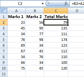
For example, We want to add the marks of two subjects entered in column A and column B and display the result in column C. Here, we will use relative reference so that the same rows of column’s A and B are added.
Steps to Use Relative Reference:
Step 1: We write the formula in any cell and press enter so that it is calculated. In this example, we write the formula(= B2 + A2) in cell C2 and press enter to calculate the formula.
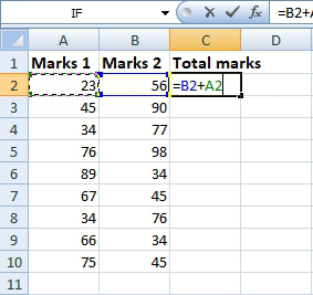
Step 2: Now click on the Fill handle at the corner of cell which contains the formula(C2).

Step 3: Drag the Fill handle up to the cells you want to fill. In our example, we will drag it till cell C10.
Step 4: Now we can see that the addition operation is performed between the cell A2 and B2, A3 and B3 and so on.
Step 5: You can double-click on any cell to check that the operation is performed in between which cells.
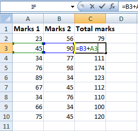
Thus, in the above example, we see that the relative address of cell A2 changes to A3, A4, and so on, similarly the relative address changes for column B, depending on the relative position of the row.
Absolute Reference
Absolute reference is the cell reference in which the row and column are made constant by adding the dollar ($) sign before the column name and row number. The absolute reference does not change as you copy the formula from one cell to other. If either the row or the column is made constant then it is known as a mixed reference. You can also press the F4 key to make any cell reference constant. $A$1, $B$3 are examples of absolute cell reference.
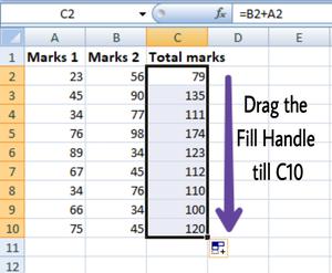
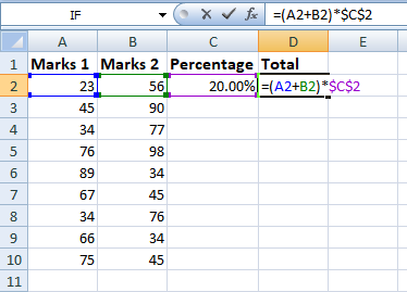
For example, We want to multiply the sum of marks of two subjects, entered in column A and column B, with the percentage entered in cell C2 and display the result in column D. Here, we will use absolute reference so that the address of cell C2 remains constant and does not change with the relative position of column and rows.
Steps to Use Absolute Reference:
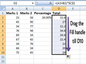
Step 1: We write the formula in any cell and press enter so that it is calculated. In this example, we write the formula(=(A2+B2)*$C$2) in cell D2 and press enter to calculate the formula.
Step 2: Now click on the Fill handle at the corner of cell which contains the formula(D2).
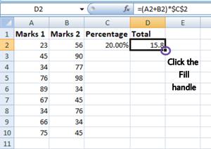
Step 3: Drag the Fill handle up to the cells you want to fill. In our example, we will drag it till cell D10.
Step 4: Now we can see that the percentage is calculated in column D.
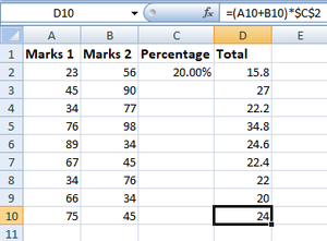
Step 5: You can double-click on any cell to check that the operation is performed in between which cells, and we see that the address of cell C2 does not change.
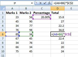
Thus, in the above example we see that the address of cell C2 is not changed whereas the address of column A and B changes with the relative position of the row and column, this happened because we used the absolute address of the cell C2.
Содержание
- Relative and Absolute Cell References in MS Excel
- Relative Reference
- Absolute Reference
- Address Function in Excel
- Address Function in Excel
- Syntax of the ADDRESS Function
- How to Use the Address Function in Excel? (With Example)
- How to Use the INDIRECT Function to Pass the Address?
- Frequently Asked Questions
- Key Takeaways
- Recommended Articles
- Absolute, Relative, and Mixed Cell References in Excel
- What are Relative Cell References in Excel?
- When to Use Relative Cell References in Excel?
- What are Absolute Cell References in Excel?
- What does the Dollar ($) sign do?
- When to Use Absolute Cell References in Excel?
- What are Mixed Cell References in Excel?
- How to Change the Reference from Relative to Absolute (or Mixed)?
Relative and Absolute Cell References in MS Excel
Cell reference is the address or name of a cell or a range of cells. It is the combination of column name and row number. It helps the software to identify the cell from where the data/value is to be used in the formula. We can reference the cell of other worksheets and also of other programs.
- Referencing the cell of other worksheets is known as External referencing.
- Referencing the cell of other programs is known as Remote referencing.
There are two types of cell references in Excel:
- Relative reference
- Absolute reference
Relative Reference
Relative reference is the default cell reference in Excel. It is simply the combination of column name and row number without any dollar ($) sign. When you copy the formula from one cell to another the relative cell address changes depending on the relative position of column and row. C1, D2, E4, etc are examples of relative cell references. Relative references are used when we want to perform a similar operation on multiple cells and the formula must change according to the relative address of column and row.
For example, We want to add the marks of two subjects entered in column A and column B and display the result in column C. Here, we will use relative reference so that the same rows of column’s A and B are added.
Steps to Use Relative Reference:
Step 1: We write the formula in any cell and press enter so that it is calculated. In this example, we write the formula(= B2 + A2) in cell C2 and press enter to calculate the formula.
Step 2: Now click on the Fill handle at the corner of cell which contains the formula(C2).
Step 3: Drag the Fill handle up to the cells you want to fill. In our example, we will drag it till cell C10.
Step 4: Now we can see that the addition operation is performed between the cell A2 and B2, A3 and B3 and so on.
Step 5: You can double-click on any cell to check that the operation is performed in between which cells.
Thus, in the above example, we see that the relative address of cell A2 changes to A3, A4, and so on, similarly the relative address changes for column B, depending on the relative position of the row.
Absolute Reference
Absolute reference is the cell reference in which the row and column are made constant by adding the dollar ($) sign before the column name and row number. The absolute reference does not change as you copy the formula from one cell to other. If either the row or the column is made constant then it is known as a mixed reference. You can also press the F4 key to make any cell reference constant. $A$1, $B$3 are examples of absolute cell reference.
For example, We want to multiply the sum of marks of two subjects, entered in column A and column B, with the percentage entered in cell C2 and display the result in column D. Here, we will use absolute reference so that the address of cell C2 remains constant and does not change with the relative position of column and rows.
Steps to Use Absolute Reference:
Step 1: We write the formula in any cell and press enter so that it is calculated. In this example, we write the formula(=(A2+B2)*$C$2) in cell D2 and press enter to calculate the formula.
Step 2: Now click on the Fill handle at the corner of cell which contains the formula(D2).
Step 3: Drag the Fill handle up to the cells you want to fill. In our example, we will drag it till cell D10.
Step 4: Now we can see that the percentage is calculated in column D.
Step 5: You can double-click on any cell to check that the operation is performed in between which cells, and we see that the address of cell C2 does not change.
Thus, in the above example we see that the address of cell C2 is not changed whereas the address of column A and B changes with the relative position of the row and column, this happened because we used the absolute address of the cell C2.
Источник
Address Function in Excel


Address Function in Excel
The ADDRESS function returns the absolute address of the cell based on a specified row and column number. The cell address is returned as a text string. For example, “=ADDRESS(1,2)” returns “$B$1.” An inbuilt function of Excel, it is categorized under the lookup and reference functions.
Table of contents
Syntax of the ADDRESS Function
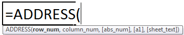
The syntax is stated as follows:
You are free to use this image on your website, templates, etc., Please provide us with an attribution link How to Provide Attribution? Article Link to be Hyperlinked
For eg:
Source: Address Function in Excel (wallstreetmojo.com)
The function accepts the following mandatory arguments:
- Row_Num: This is the row number used in the cell reference. The “row_num=1” represents row 1.
- Column_Num: This is the column number used in the cell reference. The “column_num= 2” represents column B.
The function accepts the following optional arguments:
- Abs_num (absolute number): This is the type of cell referenceCell ReferenceCell reference in excel is referring the other cells to a cell to use its values or properties. For instance, if we have data in cell A2 and want to use that in cell A1, use =A2 in cell A1, and this will copy the A2 value in A1.read more –absolute or relative. If this parameter is omitted, the default value is set at 1 (absolute). It can have any of the following values depending on the requirement:
| Abs_num | Explanation |
| 1 | Absolute referenceAbsolute ReferenceAbsolute reference in excel is a type of cell reference in which the cells being referred to do not change, as they did in relative reference. By pressing f4, we can create a formula for absolute referencing.read more like “$A$1” |
| 2 | Relative column, absolute row like “A$1” |
| 3 | Absolute column, relative row like “$A1” |
| 4 | Relative referenceRelative ReferenceIn Excel, relative references are a type of cell reference that changes when the same formula is copied to different cells or worksheets. Let’s say we have =B1+C1 in cell A1, and we copy this formula to cell B2 and it becomes C2+D2.read more like “A1” |
- A1: This is the reference style used. It can be either “A1” (1 or true) or “R1C1” (0 or false). If this parameter is omitted, the default style is “A1.”
- Sheet_text: This is the name of the sheet used in the cell address. If this parameter is omitted, no worksheet name is used.
How to Use the Address Function in Excel? (With Example)
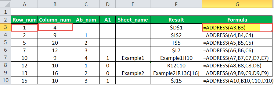
Let us consider the various possible outcomes of the ADDRESS function, as shown in the succeeding image.
The observations of a few rows are explained as follows:
1. The Third Row
- The “row=1” and “column=4.”
- The formula is “=ADDRESS(1,4).”
- By default, the parameters “absolute number” and “reference type” are set at 1.
- The result is an absolute address with an absolute row and an absolute column, i.e., “$D$1.”
- The “$D” signifies the absolute column “4” and “$1” signifies the absolute row “1.”
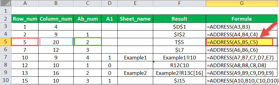
2. The Fifth Row
- The “row=5,” “column=20,” and “abs_num=2.”
- The ADDRESS formula can be rewritten in a simpler form as “=ADDRESS(5,20,2).”
- The reference style is set at 1 (true) when it has not been defined explicitly.
- The result is “T$5,” which has an absolute row ($5) and a relative column (T).
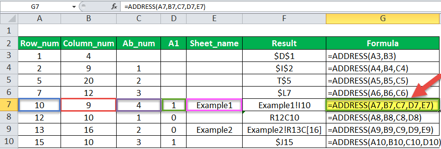
3. The Seventh Row
- We pass all the arguments of the ADDRESS function, including the optional ones.
- The “row=10,” “column=9,” “abs_num=4,” “A1=1,” and “sheet_name=Example1.”
- The address formula can be rewritten in a simpler form as “=ADDRESS(10,9,4,1,”Example1″).”
- The result is “Example1!I10.”
- Since the “absolute number” parameter is set at 4, the result is a relative reference (“I10”).
How to Use the INDIRECT Function to Pass the Address?
The reference of a cell can be derived with the help of the ADDRESS function. However, if we are interested in obtaining the value stored in the Excel address of cells, we use the INDIRECT function INDIRECT Function The INDIRECT excel function is used to indirectly refer to cells, cell ranges, worksheets, and workbooks. read more . With this function, we can get the actual value through reference.
Syntax of the INDIRECT Function
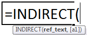
The function accepts the following arguments:
- Ref_text: This is the cell reference supplied in the form of a text string.
- A1: This is a logical value that specifies the style of reference. It can be either “A1” (true or omitted) or “R1C1” (false).
The first argument is mandatory, while the second is optional.
Let us consider an example.
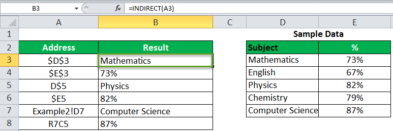
The data is given in the following image. We want to find the value of the cell reference passed in the INDIRECT function.
In the first observation, the “ADDRESS=$D$3.” We rewrite the function as “=INDIRECT(A3).”
In cell D3, under the sample data, the value is “Mathematics.” This is the same as the result of the INDIRECT function in cell B3.
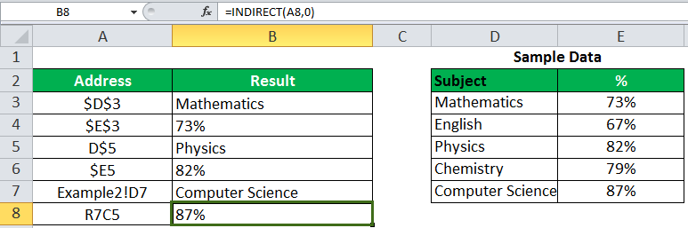
Let us consider another example in which the reference style is R7C5.
Here, we must set the “ref_type” to “false” (0), so that the INDIRECT function can read the reference style.
The output of “=INDIRECT(A8,0)” is 87%.
Frequently Asked Questions
The uses of the function are listed as follows:
– It is used to address the first or the last cell in a range.
– It helps convert a column number to a letter and vice versa.
– It is used to construct a cell reference within a formula.
– It helps find the cell value from the row and column number.
– It returns the address of the cell with the highest value.
The formula to return the full address of a named range is stated as follows:
“=ADDRESS(ROW(range), COLUMN(range)) & “:” & ADDRESS(ROW(range) + ROWS(range)-1, COLUMN(range) + COLUMNS(range)-1)”
“Range” is the named range whose address is required.
If the range address is required as a relative reference, the “abs_num” argument is set at 4. The formula can be rewritten as follows:
“=ADDRESS(ROW(range), COLUMN(range), 4) & “:” & ADDRESS(ROW(range) + ROWS(range)-1, COLUMN(range) + COLUMNS(range)-1, 4)”
Key Takeaways
- The ADDRESS function creates a cell address from a given row and column number.
- The syntax of the ADDRESS function is–“ADDRESS(row_num, column_num, [abs_num], [a1], [sheet_text]).”
- The “row_num” and “column_num” are mandatory arguments, while “abs_num,” “A1,” and “sheet_text” are optional arguments.
- The “abs_num” parameter can be set as follows:
- 1 or omitted–Absolute reference
- 2–Absolute row, relative column
- 3–Relative row, absolute column
- 4–Relative reference
- The reference style can be set at either “A1” (1 or true) or “R1C1” (0 or false).
- The default reference style is “A1.”
- The INDIRECT function helps obtain the value stored in the Excel address of cells. The syntax of the INDIRECT function is–“INDIRECT(ref_text, [a1]).”
Recommended Articles
This has been a guide to Address Excel Function. Here we discuss how to use the Address Formula in Excel along with step by step examples and downloadable Excel templates.`
Источник
Absolute, Relative, and Mixed Cell References in Excel
A worksheet in Excel is made up of cells. These cells can be referenced by specifying the row value and the column value.
For example, A1 would refer to the first row (specified as 1) and the first column (specified as A). Similarly, B3 would be the third row and second column.
The power of Excel lies in the fact that you can use these cell references in other cells when creating formulas.
Now there are three kinds of cell references that you can use in Excel:
- Relative Cell References
- Absolute Cell References
- Mixed Cell References
Understanding these different types of cell references will help you work with formulas and save time (especially when copy-pasting formulas).
This Tutorial Covers:
What are Relative Cell References in Excel?
Let me take a simple example to explain the concept of relative cell references in Excel.
Suppose I have a data set shown below:
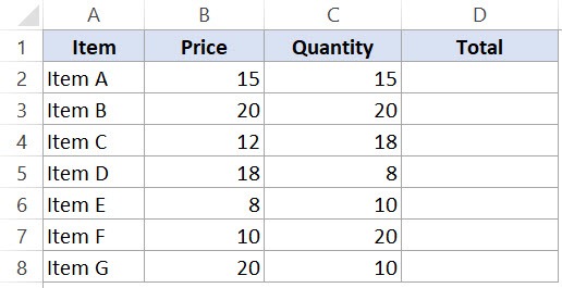
To calculate the total for each item, we need to multiply the price of each item with the quantity of that item.
For the first item, the formula in cell D2 would be B2* C2 (as shown below):
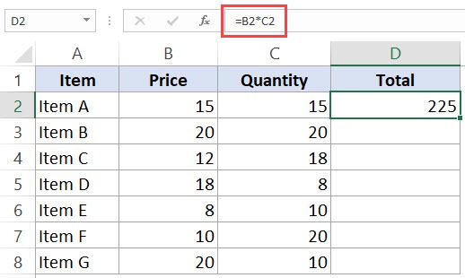
Now, instead of entering the formula for all the cells one by one, you can simply copy cell D2 and paste it into all the other cells (D3:D8). When you do it, you will notice that the cell reference automatically adjusts to refer to the corresponding row. For example, the formula in cell D3 becomes B3*C3 and the formula in D4 becomes B4*C4.
These cell references that adjust itself when the cell is copied are called relative cell references in Excel.
When to Use Relative Cell References in Excel?
Relative cell references are useful when you have to create a formula for a range of cells and the formula needs to refer to a relative cell reference.
In such cases, you can create the formula for one cell and copy-paste it into all cells.
What are Absolute Cell References in Excel?
Unlike relative cell references, absolute cell references don’t change when you copy the formula to other cells.
For example, suppose you have the data set as shown below where you have to calculate the commission for each item’s total sales.
The commission is 20% and is listed in cell G1.
![]()
To get the commission amount for each item sale, use the following formula in cell E2 and copy for all cells:
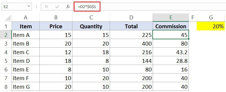
Note that there are two dollar signs ($) in the cell reference that has the commission – $G$2.
What does the Dollar ($) sign do?
A dollar symbol, when added in front of the row and column number, makes it absolute (i.e., stops the row and column number from changing when copied to other cells).
For example, in the above case, when I copy the formula from cell E2 to E3, it changes from =D2*$G$1 to =D3*$G$1.
Note that while D2 changes to D3, $G$1 doesn’t change.
Since we have added a dollar symbol in front of ‘G’ and ‘1’ in G1, it wouldn’t let the cell reference change when it’s copied.
Hence this makes the cell reference absolute.
When to Use Absolute Cell References in Excel?
Absolute cell references are useful when you don’t want the cell reference to change as you copy formulas. This could be the case when you have a fixed value that you need to use in the formula (such as tax rate, commission rate, number of months, etc.)
While you can also hard code this value in the formula (i.e., use 20% instead of $G$2), having it in a cell and then using the cell reference allows you to change it at a future date.
For example, if your commission structure changes and you’re now paying out 25% instead of 20%, you can simply change the value in cell G2, and all the formulas would automatically update.
What are Mixed Cell References in Excel?
Mixed cell references are a bit more tricky than the absolute and relative cell references.
There can be two types of mixed cell references:
- The row is locked while the column changes when the formula is copied.
- The column is locked while the row changes when the formula is copied.
Let’s see how it works using an example.
Below is a data set where you need to calculate the three tiers of commission based on the percentage value in cell E2, F2, and G2.
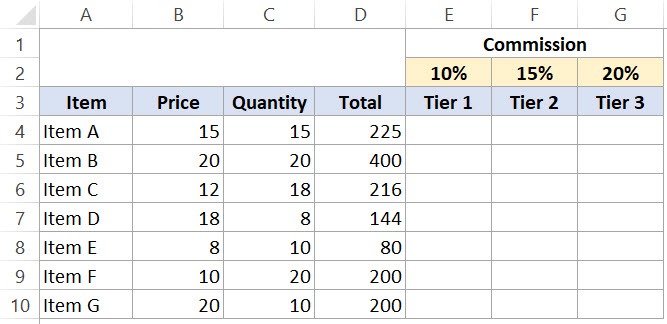
Now you can use the power of mixed reference to calculate all these commissions with just one formula.
Enter the below formula in cell E4 and copy for all cells.
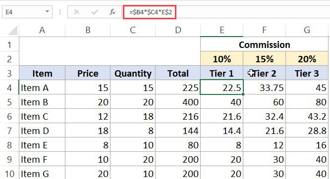
The above formula uses both kinds of mixed cell references (one where the row is locked and one where the column is locked).
Let’s analyze each cell reference and understand how it works:
- $B4 (and $C4) – In this reference, the dollar sign is right before the Column notation but not before the Row number. This means that when you copy the formula to the cells on the right, the reference will remain the same as the column is fixed. For example, if you copy the formula from E4 to F4, this reference would not change. However, when you copy it down, the row number would change as it is not locked.
- E$2 – In this reference, the dollar sign is right before the row number, and the Column notation has no dollar sign. This means that when you copy the formula down the cells, the reference will not change as the row number is locked. However, if you copy the formula to the right, the column alphabet would change as it’s not locked.
How to Change the Reference from Relative to Absolute (or Mixed)?
To change the reference from relative to absolute, you need to add the dollar sign before the column notation and the row number.
For example, A1 is a relative cell reference, and it would become absolute when you make it $A$1.
If you only have a couple of references to change, you may find it easy to change these references manually. So you can go to the formula bar and edit the formula (or select the cell, press F2, and then change it).
However, a faster way to do this is by using the keyboard shortcut – F4.
When you select a cell reference (in the formula bar or in the cell in edit mode) and press F4, it changes the reference.
Suppose you have the reference =A1 in a cell.
Here is what happens when you select the reference and press the F4 key.
- Press F4 key once: The cell reference changes from A1 to $A$1 (becomes ‘absolute’ from ‘relative’).
- Press F4 key two times: The cell reference changes from A1 to A$1 (changes to mixed reference where the row is locked).
- Press F4 key three times: The cell reference changes from A1 to $A1 (changes to mixed reference where the column is locked).
- Press F4 key four times: The cell reference becomes A1 again.
You May Also Like the Following Excel Tutorials:
Источник