
Convert numbers stored as text to numbers
Excel for Microsoft 365 Excel for Microsoft 365 for Mac Excel 2021 Excel 2021 for Mac Excel 2019 Excel 2019 for Mac Excel 2016 Excel 2016 for Mac Excel 2013 Excel Web App Excel 2010 Excel 2007 Excel for Mac 2011 Excel Starter 2010 More…Less
Numbers that are stored as text can cause unexpected results, like an uncalculated formula showing instead of a result. Most of the time, Excel will recognize this and you’ll see an alert next to the cell where numbers are being stored as text. If you see the alert, select the cells, and then click  to choose a convert option.
Check out Format numbers to learn more about formatting numbers and text in Excel.

If the alert button is not available, do the following:
1. Select a column
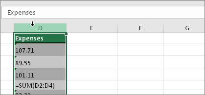
Select a column with this problem. If you don’t want to convert the whole column, you can select one or more cells instead. Just be sure the cells you select are in the same column, otherwise this process won’t work. (See «Other ways to convert» below if you have this problem in more than one column.)
2. Click this button
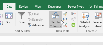
The Text to Columns button is typically used for splitting a column, but it can also be used to convert a single column of text to numbers. On the Data tab, click Text to Columns.
3. Click Apply
The rest of the Text to Columns wizard steps are best for splitting a column. Since you’re just converting text in a column, you can click Finish right away, and Excel will convert the cells.
4. Set the format

Press CTRL + 1 (or  + 1 on the Mac). Then select any format.
Note: If you still see formulas that are not showing as numeric results, then you may have Show Formulas turned on. Go to the Formulas tab and make sure Show Formulas is turned off.
Other ways to convert:
You can use the VALUE function to return just the numeric value of the text.
1. Insert a new column
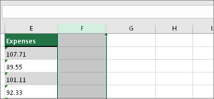
Insert a new column next to the cells with text. In this example, column E contains the text stored as numbers. Column F is the new column.
2. Use the VALUE function
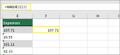
In one of the cells of the new column, type =VALUE() and inside the parentheses, type a cell reference that contains text stored as numbers. In this example it’s cell E23.
3. Rest your cursor here
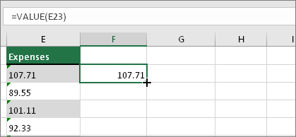
Now you’ll fill the cell’s formula down, into the other cells. If you’ve never done this before, here’s how to do it: Rest your cursor on the lower-right corner of the cell until it changes to a plus sign.
4. Click and drag down
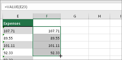
Click and drag down to fill the formula to the other cells. After that’s done, you can use this new column, or you can copy and paste these new values to the original column. Here’s how to do that: Select the cells with the new formula. Press CTRL + C. Click the first cell of the original column. Then on the Home tab, click the arrow below Paste, and then click Paste Special > Values.
If the steps above didn’t work, you can use this method, which can be used if you’re trying to convert more than one column of text.
-
Select a blank cell that doesn’t have this problem, type the number 1 into it, and then press Enter.
-
Press CTRL + C to copy the cell.
-
Select the cells that have numbers stored as text.
-
On the Home tab, click Paste > Paste Special.
-
Click Multiply, and then click OK. Excel multiplies each cell by 1, and in doing so, converts the text to numbers.
-
Press CTRL + 1 (or
 + 1 on the Mac). Then select any format.

Related topics
Replace a formula with its result
Top ten ways to clean your data
CLEAN function
Need more help?
Want more options?
Explore subscription benefits, browse training courses, learn how to secure your device, and more.
Communities help you ask and answer questions, give feedback, and hear from experts with rich knowledge.
Skip to content
В этом руководстве показано множество различных способов преобразования текста в число в Excel: опция проверки ошибок в числах, формулы, математические операции, специальная вставка и многое другое.
Иногда значения в ваших таблицах Excel выглядят как числа, но их нельзя сложить или перемножить, они приводят к ошибкам в формулах. Общая причина этого — числа, записанные как текст. Во многих случаях Microsoft Excel достаточно умен, чтобы автоматически преобразовывать цифровые символы, импортированные из других программ, в обычные числа. Но иногда числа остаются отформатированными в виде текста, что вызывает множество проблем в ваших электронных таблицах.
Перестает правильно работать сортировка данных, поскольку числовые и текстовые значения упорядочиваются по-разному. Функции поиска, подобные ВПР, также не могут найти нужные значения (подробнее об этом читайте – Почему не работает ВПР?). Подсчет по условиям СУММЕСЛИ и СЧЁТЕСЛИ даст неверные результаты. Если они находятся среди «нормальных» чисел, то функция СУММ их проигнорирует, а вы этого даже не заметите. В результате – неверные расчеты.
- Как выглядят числа-как текст?
- Используем индикатор ошибок.
- Изменение формата ячейки может преобразовать текст в число
- Специальная вставка
- Инструмент «текст по столбцам»
- Повторный ввод
- Формулы для преобразования текста в число
- Как можно использовать математические операции
- Удаление непечатаемых символов
- Использование макроса VBA
- Как извлечь число из текста при помощи инструмента Ultimate Suite
Из этого материала вы узнаете, как преобразовать строки в «настоящие» числа.
Как определить числа, записанные как текст?
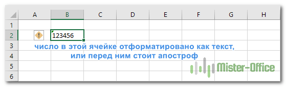
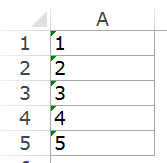
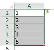
В Excel есть встроенная функция проверки ошибок, которая предупреждает вас о возможных проблемах со значениями ячеек. Это выглядит как маленький зеленый треугольник в верхнем левом углу ячейки. При выборе ячейки с таким индикатором ошибки отображается предупреждающий знак с желтым восклицательным знаком (см. Скриншот ниже). Наведите указатель мыши на этот знак, и Excel сообщит вам о потенциальной проблеме: в этой ячейке число сохранено как текст или перед ним стоит апостроф .
В некоторых случаях индикатор ошибки не отображается для чисел, записанных в виде текста. Но есть и другие визуальные индикаторы текстовых чисел:
|
Число |
Строка (текстовое значение) |
• Если выбрано несколько ячеек, в строке состояния отображается «Среднее», «Количество» и «Сумма» . |
• Если выбрано несколько ячеек, строка состояния показывает только Количество . • В поле Числовой формат отображается текстовый формат (во многих случаях, но не всегда). • В строке формул может быть виден начальный апостроф. • Зелёный треугольник в левом верхнем углу. |
На изображении ниже вы можете видеть текстовые представления чисел справа и реальные числа слева:
Есть несколько разных способов изменить текст на число Excel. Ниже мы рассмотрим их, начиная с самых быстрых и простых. Если простые методы не работают для вас, пожалуйста, не расстраивайтесь. Нет проблем, которые невозможно преодолеть. Просто нужно попробовать другие способы.
Используем индикатор ошибок.
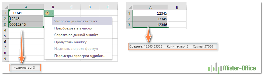
Если в ваших клетках отображается индикатор ошибки (зеленый треугольник в верхнем левом углу), преобразование выполняется одним щелчком мыши:
- Выберите всю область, где цифры сохранены как текст.
- Нажмите предупреждающий знак и затем — Преобразовать в число.

Таким образом можно одним махом преобразовать в числа весь столбец. Просто выделите всю проблемную область, а затем жмите восклицательный знак.
Смена формата ячейки.
Все ячейки в Экселе имеют определенный формат, который указывает программе, как их обрабатывать. Например, даже если в клетке таблицы будут записаны цифры, но формат выставлен текстовый, то они будут рассматриваться как простой текст. Никакие подсчеты с ними вы провести не сможете. Для того, чтобы Excel воспринимал цифры как нужно, они должны быть записаны с общим или числовым форматом.
Итак, первый быстрый способ видоизменения заключается в следующем:
- Выберите ячейки с цифрами в текстовом формате.
- На вкладке «Главная » в группе «Число» выберите « Общий» или « Числовой» в раскрывающемся списке «Формат» .

Или же можно воспользоваться контекстным меню, вызвав его правым кликом мышки.

Последовательность действий в этом случае показана на рисунке. В любом случае, нужно применить числовой либо общий формат.
Этот способ не слишком удобен и достался нам «в наследство» от предыдущих версий Excel, когда еще не было индикатора ошибки в виде зелёного уголка.
Примечание. Этот метод не работает в некоторых случаях. Например, если вы примените текстовый формат, запишете несколько цифр, а затем измените формат на «Числовой». Тут ячейка все равно останется отформатированной как текст.
То же самое произойдёт, если перед цифрами будет стоять апостроф. Это однозначно указывает Excel, что записан именно текст и ничто другое.
Совет. Если зеленых уголков нет совсем, то проверьте — не выключены ли они в настройках вашего Excel (Файл — Параметры — Формулы — Числа, отформатированные как текст или с предшествующим апострофом).
Специальная вставка.
По сравнению с предыдущими методами этот метод требует еще нескольких дополнительных шагов, но работает почти на 100%.
Чтобы исправить числа, отформатированные как текст с помощью специальной вставки, выполните следующие действия:
- Выделите клетки таблицы с текстовым номером и установите для них формат «Общий», как описано выше.
- Скопируйте какую-нибудь пустую ячейку. Для этого либо установите в нее курсор и нажмите
Ctrl + C, либо щелкните правой кнопкой мыши и выберите «Копировать» в контекстном меню. - Выберите клетки таблицы, которые вы хотите трансформировать, щелкните правой кнопкой мыши и выберите «Специальная вставка». В качестве альтернативы, нажмите комбинацию клавиш
Ctrl + Alt + V. - В диалоговом окне «Специальная вставка» выберите «Значения» в разделе «Вставить» и затем «Сложить» в разделе «Операция».
- Нажмите ОК.

Если все сделано правильно, то ваши значения изменят выравнивание слева на правую сторону. Excel теперь воспринимает их как числа.
Инструмент «текст по столбцам».
Это еще один способ использовать встроенные возможности Excel. При использовании для других целей, например для разделения ячеек, мастер «Текст по столбцам» представляет собой многоэтапный процесс. А вот чтобы просто выполнить нашу метаморфозу, нажимаете кнопку Готово на самом первом шаге 
- Выберите позиции (можно и весь столбец), которые вы хотите конвертировать, и убедитесь, что их формат установлен на Общий.
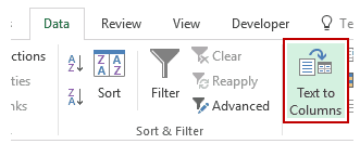
- Перейдите на вкладку «Данные», группу «Инструменты данных» и нажмите кнопку «Текст по столбцам» .
- На шаге 1 мастера распределения выберите «С разделителями» в разделе «Формат исходных данных» и сразу чтобы завершить преобразование, нажмите «Готово» .

Это все, что нужно сделать!
Повторный ввод.
Если проблемных ячеек, о которых мы ведём здесь разговор, у вас не очень много, то, возможно, неплохим вариантом будет просто ввести их заново.
Для этого сначала установите их формат на «Обычный». Затем в каждую из них введите цифры заново.
Думаю, вы знаете, как корректировать ячейку — либо двойным кликом мышки, либо через клавишу F2.
Но это, конечно, если таких «псевдо-чисел» немного. Иначе овчинка не стоит выделки. Есть много других менее трудоемких способов.
Преобразовать текст в число с помощью формулы
До сих пор мы обсуждали встроенные возможности, которые можно применить для перевода текста в число в Excel. Во многих ситуациях это может быть сделано быстрее с помощью формулы.
В Microsoft Excel есть специальная функция — ЗНАЧЕН (VALUE в английском варианте). Она обрабатывает как текст в кавычках, так и ссылку на элемент таблицы, содержащий символы для трансформирования.
Функция ЗНАЧЕН может даже распознавать набор цифр, включающих некоторые «лишние» символы.
Например, распознает цифры, записанные с разделителем тысяч в виде пробела:
=ЗНАЧЕН(«1 000»)
Конвертируем число, введенное с символом валюты и разделителем тысяч:
=ЗНАЧЕН(«1 000 $»)
Обе эти формулы возвратят число 1000.
Точно так же она расправляется с пробелами перед цифрами.

Чтобы преобразовать столбец символьных значений в числа, введите выражение в первую позицию и перетащите маркер заполнения, чтобы скопировать его вниз по столбцу.
Функция ЗНАЧЕН также пригодится, когда вы извлекаете что-либо из символьной строки с помощью одной из текстовых функций, таких как ЛЕВСИМВ, ПРАВСИМВ и ПСТР.
Например, чтобы получить последние 3 символа из A2 и вернуть результат в виде цифр, используйте следующее:
=ЗНАЧЕН(ПРАВСИМВ(A2;3))
На приведенном ниже рисунке продемонстрирована формула трансформации:

Если вы не обернете функцию ПРАВСИМВ в ЗНАЧЕН, результат будет возвращен в виде набора символов, что делает невозможным любые вычисления с извлеченными значениями.
Этот метод подходит, когда вы точно знаете, сколько символов и откуда вы желаете получить, а затем превратить их в число.
Математические операции.
Еще один способ — выполнить простую арифметическую операцию, которая фактически не меняет исходное значение. В этом случае программа, если есть такая возможность, сама сделает нужную конвертацию.
Что это может быть? Например, сложение с нулём, умножение или деление на 1.
=A2+0
=A2*1
=A2/1

Важно, чтобы эти действия не изменили величины чисел. Выше вы видите пример таких операций: двойное умножение на минус 1, умножение на 1, сложение с 0. Наиболее элегантно и просто для ввода выглядит «двойное отрицание»: ставим два минуса перед ссылкой, то есть дважды умножаем на минус 1. Результат расчета не изменится, а записать такую формулу очень просто.
Но если исходные значения отформатированы как текст, Excel также может автоматически применить соответствующий формат и к полученным результатам. Вы сможете заметить это по выровненному влево их содержимому. Чтобы это исправить, обязательно установите общий формат для ячеек, которые используются в формуле.
Примечание. Если вы хотите, чтобы результаты были значениями, а не формулами, используйте после применения этого метода функцию специальной вставки, чтобы заменить их результатами.
Удаление непечатаемых символов.
Когда вы копируете в таблицу Excel данные из других приложений при помощи буфера обмена (то есть Копировать – Вставить), вместе с цифрами часто копируется и различный «мусор». Так в таблице могут появиться внешне не видимые непечатаемые символы. В результате ваши цифры будут восприниматься программой как символьная строка.
Эту напасть можно удалить программным путем при помощи формулы. Аналогично предыдущему примеру, в С2 можно записать примерно такое выражение:
=ЗНАЧЕН(СЖПРОБЕЛЫ(ПЕЧСИМВ(A2)))
Поясню, как это работает. Функция ПЕЧСИМВ удаляет непечатаемые знаки. СЖПРОБЕЛЫ – лишние пробелы. Функция ЗНАЧЕН, как мы уже говорили ранее, преобразует текст в число.
Макрос VBA.
Если вам часто приходится преобразовывать большие области данных из текстового формата в числовой, то есть резон для этих повторяющихся операций создать специальный макрос, который будет использоваться при необходимости. Но для того, чтобы это выполнить, прежде всего, нужно в Экселе включить макросы и панель разработчика, если это до сих пор не сделано. Нажмите правой кнопкой мыши на ленте и настройте показ этого раздела.
Нажмите сочетание клавиш Alt+F11 или откройте вкладку Разработчик (Developer) и нажмите кнопку Visual Basic. В появившемся окне редактора добавьте новый модуль через меню Insert — Module и скопируйте туда следующее небольшое выражение:
Sub Текст_в_число()
   Dim rArea As Range
   On Error Resume Next
   ActiveWindow.RangeSelection.SpecialCells(xlCellTypeConstants).Select
   If Err Then Exit Sub
   With Application: .ScreenUpdating = False: .EnableEvents = False: .Calculation = xlManual: End With
   For Each rArea In Selection.Areas
   rArea.Replace ",", "."
   rArea.FormulaLocal = rArea.FormulaLocal
   Next rArea
   With Application: .ScreenUpdating = True: .EnableEvents = True: .Calculation = xlAutomatic: End With
End Sub
После этого закрываем редактор, выполнив нажатие стандартной кнопки закрытия в верхнем правом углу окна.
Что делает этот макрос?
Вы можете выделить несколько областей данных для конвертации (можно использовать мышку при нажатой клавише CTRL). При этом, если в ваших числах в качестве разделителя десятичных разрядов используется запятая, то она будет автоматически заменена на точку. Ведь в Windows чаще всего именно точка отделяет целую и дробную части числа. А при экспорте данных из других программ запятая в этой роли встречается почему-то очень часто.
Чтобы использовать этот код, выделяем область на рабочем листе, которую нужно преобразовать. Жмем на значок «Макросы», который расположен на вкладке «Разработчик» в группе «Код». Или нам поможет комбинация клавиш ALT+F8.
Открывается окно имеющихся макросов. Находим «Текст_в_число», указываем на его и жмем на кнопку «Выполнить».
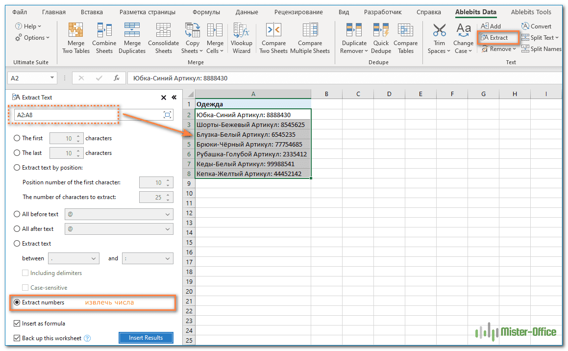
Извлечь число из текстовой строки с помощью Ultimate Suite
Как вы уже убедились, не существует универсальной формулы Excel для извлечения числа из текстовой строки. Если у вас возникли трудности с пониманием формул или их настройкой для ваших наборов данных, вам может понравиться этот простой способ получить число из строки в Excel.
Надстройка Ultimate Suite предоставляет множество инструментов для работы с текстовыми значениями: удалить лишние пробелы и ненужные символы, изменить регистр текста, подсчитать символы и слова, добавить один и тот же текст в начало или конец всех ячеек в диапазоне, преобразовать текст в числа, разделить его по отдельным ячейкам, заменить ошибочные символы с правильными.
Вот как вы можете быстро получить число из любой буквенно-цифровой строки:
- Перейдите на вкладку Ablebits Data > Текст и нажмите Извлечь (Extract) :

- Выделите все ячейки с нужным текстом.
- На панели инструмента установите переключатель «Извлечь числа (Extract numbers)».
- В зависимости от того, хотите ли вы, чтобы результаты были формулами или значениями, выберите переключатель «Вставить как формулу (Insert as formula)» или оставьте его неактивным (по умолчанию).
Я советую активировать эту возможность, если вы хотите, чтобы извлеченные числа обновлялись автоматически, как только в исходные строки вносятся какие-либо изменения.
Если вы хотите, чтобы результаты не зависели от исходных строк (например, если вы планируете удалить исходные данные позже), не выводите результат в виде формулы.
- Нажмите кнопку «Вставить результаты (Insert results)». Вот и всё!

Как и в предыдущем примере, результаты извлечения являются числами , что означает, что вы можете подсчитывать, суммировать, усреднять или выполнять любые другие вычисления с ними.
В этом примере мы решили вставить результаты как формулы , и надстройка сделала именно то, что было запрошено:
=ЕСЛИ(МИН(НАЙТИ({0;1;2;3;4;5;6;7;8;9},A2&»_0123456789″))>ДЛСТР(A2), «»,СУММПРОИЗВ(ПСТР(0&A2,НАИБОЛЬШИЙ(ИНДЕКС(ЕЧИСЛО(—ПСТР(A2,СТРОКА(ДВССЫЛ(«$1:$»&ДЛСТР(A2))),1))*СТРОКА(ДВССЫЛ(«$1:$»&ДЛСТР(A2))),0),СТРОКА(ДВССЫЛ(«$1:$»&ДЛСТР(A2))))+1,1)*10^СТРОКА(ДВССЫЛ(«$1:$»&ДЛСТР(A2)))/10))
Сложновато самому написать такую формулу, не правда ли?
Если отсутствует флажок «Вставить как формулу», вы увидите число в строке формул.
Любопытно попробовать? Просто скачайте пробную версию Ultimate Suite и убедитесь сами
Если вы хотите иметь этот, а также более 60 других полезных инструментов в своем Excel, воспользуйтесь этой специальной возможностью покупки, которую предоставлена исключительно читателям нашего блога.
Вот как вы можете преобразовать текст в число Excel с помощью формул и встроенных функций. Более сложные случаи, когда в ячейке находятся одновременно и буквы, и цифры, мы рассмотрим в отдельной статье. Я благодарю вас за чтение и надеюсь не раз еще увидеть вас в нашем блоге!
Также рекомендуем:
 Как быстро посчитать количество слов в Excel — В статье объясняется, как подсчитывать слова в Excel с помощью функции ДЛСТР в сочетании с другими функциями Excel, а также приводятся формулы для подсчета общего количества или конкретных слов в…
  Как быстро извлечь число из текста в Excel — В этом кратком руководстве показано, как можно быстро извлекать число из различных текстовых выражений в Excel с помощью формул или специального инструмента «Извлечь». Проблема выделения числа из текста возникает достаточно…
  Как умножить число на процент и прибавить проценты — Ранее мы уже научились считать проценты в Excel. Рассмотрим несколько случаев, когда известная нам величина процента помогает рассчитать различные числовые значения. Чему равен процент от числаКак умножить число на процентКак…
  Как считать проценты в Excel — примеры формул — В этом руководстве вы познакомитесь с быстрым способом расчета процентов в Excel, найдете базовую формулу процента и еще несколько формул для расчета процентного изменения, процента от общей суммы и т.д.…
  Функция ПРАВСИМВ в Excel — примеры и советы. — В последних нескольких статьях мы обсуждали различные текстовые функции. Сегодня наше внимание сосредоточено на ПРАВСИМВ (RIGHT в английской версии), которая предназначена для возврата указанного количества символов из крайней правой части…
  Функция ЛЕВСИМВ в Excel. Примеры использования и советы. — В руководстве показано, как использовать функцию ЛЕВСИМВ (LEFT) в Excel, чтобы получить подстроку из начала текстовой строки, извлечь текст перед определенным символом, заставить формулу возвращать число и многое другое. Среди…
  5 примеров с функцией ДЛСТР в Excel. — Вы ищете формулу Excel для подсчета символов в ячейке? Если да, то вы, безусловно, попали на нужную страницу. В этом коротком руководстве вы узнаете, как использовать функцию ДЛСТР (LEN в английской версии)…
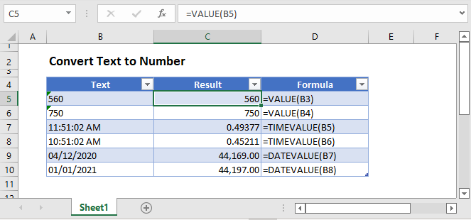
Summary
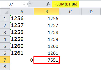
To convert simple text values to numbers, you can use the the VALUE function, or simply add zero as described below. In the example shown, the formula in C5 is:
=VALUE(B5)
Background
Sometimes Excel ends up with text in a cell, when you really want a number. There are many reasons this might happen, and many ways to fix. This article describes a formula-based approach convert text values to numbers.
Generic formula
Explanation
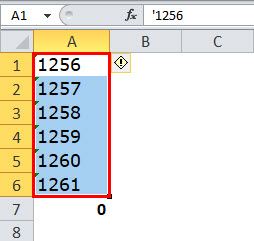
In this example, the values in column A are «stored as text». This means if you try to SUM column A, you’ll get a result of zero.
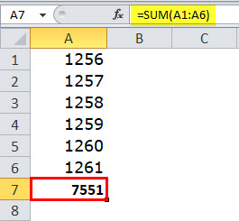
The VALUE function will try to «coerce» a number stored as text to a true number. In simple cases, it will just work and you’ll get a numeric result. If it doesn’t work, you’ll get a #VALUE error.
Add zero instead
Another common trick is to simply add zero to the text value with a formula like this:
=A1+0
This forces Excel to try and convert the text value to a number to handle the math operation. This has the same functionality as VALUE above. In the example shown, C7 uses this formula.
Stripping other characters
If a cell contains non-numeric characters like dashes, punctuation, and so on, you’ll need to remove those characters before you can convert to numbers.
The formulas in C8 and C9 show how to use the LEFT and RIGHT functions to strip non-numeric characters from a text value before it’s converted to a number. You can also use the MID function in more complicated situations. If you need to strip extra spaces or other non-printing characters, see the TRIM and CLEAN functions.
Finally, the SUBSTITUTE function will let you remove characters with «search and replace» type functionality.

Author![]()
Dave Bruns
Hi — I’m Dave Bruns, and I run Exceljet with my wife, Lisa. Our goal is to help you work faster in Excel. We create short videos, and clear examples of formulas, functions, pivot tables, conditional formatting, and charts.
This is the best learning resource I have stumbled upon in many years during the process of my Excel learning.
Get Training
Quick, clean, and to the point training
Learn Excel with high quality video training. Our videos are quick, clean, and to the point, so you can learn Excel in less time, and easily review key topics when needed. Each video comes with its own practice worksheet.
View Paid Training & Bundles
Help us improve Exceljet
This post is going to show you all the ways you can convert text to numbers in Microsoft Excel.
An issue that comes up quite often in Excel is numbers that have been entered or formatted as text values.
This can cause many headaches when trying to troubleshoot why a formula like a SUM is not giving the correct answer.
Even though the data looks like a number, it can actually be a text value and will be ignored from any numerical calculations like a sum.
In this post, I will show you how you can identify such numbers which are stored as text values, and 7 ways you can use to convert the text into a proper number value.
How to Indentify Numbers Entered as Text
How can you tell if your number data has been entered as text?
There are quite a few easy ways to tell!
Left Aligned
The first way you might be able to tell if you have text values instead of numerical values is the way the data is aligned in the cell.
By default text is left aligned and numbers are right aligned.
Unless the alignment formatting has been changed from the default, this will be an easy way to spot numbers that have been formatted as text.
Green Triangle Error Checking
If you don’t realize you have numbers entered as text values, it can potentially cause some serious errors. This is why it’s flagged by Excel’s built-in error checker.
Any cells that are flagged with an error will show a small green triangle in the left of the cell to visually indicate an error.
When you select such a cell a small warning icon will appear.
When you click on this, it will show you what the error is. In this case, you can see the error is Number Stored as Text.
You can turn off this error checking entirely, or customize which errors are flagged.
Go to the File tab and then select Options at the bottom. This will open up the Excel Options menu.
In the Formula section of the Excel Options menu ➜ Error Checking.
Uncheck the Enable background error checking option to disable this feature. You can also customize the color used to indicate errors here.
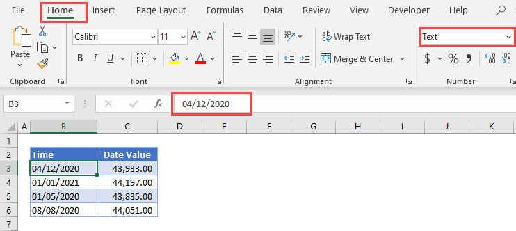
Text Format Applied
One way that numbers get entered as text is when the cell has been formatted as text. This causes values to be entered as text values regardless of whether they are numerical.
There is a quick way to determine whether or not a cell has had text formatting applied.
Select the cell and go to the Home tab. You will be able to see if Text is the selected formatting in the dropdown menu found in the Number section of the ribbon.
Preceding Apostrophe
Another way that numbers can be entered as text is by using a preceding apostrophe.
When you enter an apostrophe ' as the first character in a cell, anything after will be regarded as a text value by Excel.
This means if you see a leading apostrophe in the formula bar, you know the data is a text value.
Use the ISTEXT Function
Excel has a function you can use to test if a value is a text value or not.
ISTEXT ( input )- input is the value, cell or range which you want to test if it is text.
The ISTEXT function will return TRUE if the value is text and FALSE otherwise.
= ISTEXT ( B3 )Here you can see the ISTEXT function being used to determine if the cells contain text. The function returns TRUE when it finds a text value.
ISNUMBER ( input )- input is the value, cell or range which you want to test if it is a number.
Similarly, you can test if a value is a number using the ISNUMBER function. It takes a single input and returns TRUE when the value is a number and FALSE otherwise.
Here the same data is tested using the ISNUMBER function. The function returns FALSE when it does not find a number.
Status Bar Only Shows a Count
Another way to quickly test a range of cells to see if they are all text is by using the status bar.
When you select a range of numerical values, Excel will show you some basic statistics like the sum, min, max, and average in the status bar.
If they are all numbers entered as text values, then these basic statistics won’t be calculated. Instead, you will only see the count of the cells in the status bar.
Note: If just one of the cells is a numerical value, you will see the full set of statistics in the status bar.
Convert Text to Number with Error Checking
You have already seen that you can use error checking to spot numbers entered as text.
The error checking will also allow you to convert these text values into proper numbers.
Click on the Error icon and choose Convert to Number from the options. Excel will then convert each cell in the selected range into a number.
Note: This option can be very slow when you have a large number of cells to convert.
Convert Text to Number with Text to Column
Usually, Text to Columns is for splitting data into multiple columns. But with this trick, you can use it to convert text format into the general format.
Text to Column will let you choose a delimiter character to split your data based on. If you deselect this option and don’t pick any delimiter then it won’t split your data.
You are then able to choose how to format the results, and this is where you can choose a general format for the output.
Follow these steps to use the text to column feature to convert text to numbers.
- Select the cells that contain the text which you want to convert into number.
- Go to the Data tab.
- Click on the Text to Column command found in the Data Tools tab.
- Select Delimited in the Original data type options.
- Press the Next button.
- Press the Next button again in step 2 of the Convert Text to Columns wizard. You can keep the default options.
- Select General from the Column data format option.
- Select a Destination if you want to place the converted values in a new location. Otherwise you can keep the default value which should be the active cell, this will replace the text with numeric values.
- Press the Finish button.
This will convert your text values into numerical values.
The Text to Column command is usually used to split comma-separated or other delimiter separated data into multiple columns.
Any delimited data will be text data, so when Excel splits the data into multiple columns it also converts numerical data into numbers for added convenience.
This is also true even if there is nothing to split!
So the Text to Column wizard can be used to converts numerical text values to numbers.
Convert Text to Number with Multiply by 1
Even when values are stored as text you can still perform certain numerical calculations with them and the results of these calculations will also be numerical values.
You can use this to convert the text into numbers by multiplying them by 1. Since you are multiplying by 1, it won’t change the numbers but it will convert them.
= B3 * 1You can use the above formula in an adjacent cell and copy and paste it down to convert an entire column.
If you want to remove the formula after, you can copy and paste them as values.
Convert Text to Number with Paste Special Multiply
Multiplying by 1 is a great trick for converting text to values, but you might not want to use a formula for this.
The great news is there is an easy way to multiply your text by 1 without using a formula.
This means you can convert your text in place and you don’t need to copy and paste formulas as values in an additional step.
You can use Paste Special Multiply to convert your text values. Follow these steps to multiply by 1 using Paste Special.
- Enter 1 into a cell elsewhere in the sheet. The 1 doesn’t even need to be a number value and can be a text value.
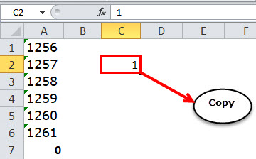
- Copy the cell which contains 1 using Ctrl + C on your keyboard or right click and choose Copy.
- Select the cells with the text values to convert.
- Press Ctrl + Alt + V on your keyboard or right click and choose Paste Special. This will open up the Paste Special menu.
- Select Values under the Paste options and select Multiply under the Operation options.
- Press the OK button.
This will multiply all the values by 1 which was the value in the copied cell. As a result, the text is converted into values, but since you are multiplying by 1 the numbers won’t change.
Convert Text to Number with VALUE Function
There is actually a dedicated function you can use for converting text to numerical values.
The VALUE function takes a text value and returns the text value as a number.
= VALUE ( text )- text is the text value you want to convert into a numerical value.
If the text contains any non-numerical characters, then the VALUE function will return a #VALUE! error. It doesn’t extract numbers from text, it can only convert numbers entered as text into numbers.
= VALUE ( B3 )You can use the above formula to convert the text in cell B3 into a number and then copy and paste the formula to convert the entire column.
Convert Text to Number with Power Query
Power Query is an amazing tool for any type of data transformation required. It can certainly be used to convert text into numbers as well.
Power Query is strongly typed. This means calculations with incompatible data types will result in an error. So you won’t be able to multiply text values by 1 to convert them into numbers.
But Power Query does come with an easy way to convert data types, including text to numbers.
Follow these steps once your data has been imported into Power Query.
Click on the data type icon to the left side of the column heading for the values you want to convert.
Each column in the Power Query editor has a data type icon that displays the current data type of the column. If the column has not been assigned a data type, then the icon shown will be ABC123.
There are several numeric data types available in Power Query and which one you choose will depend on the level of decimal precision you need.
In this case, you can select the Whole Number option from the menu.
Notice the values in the column are now right-aligned and the data type icon has changed? These are visual indicators that the data type is now whole numbers instead of text.
= Table.TransformColumnTypes(Source,{{"Text", Int64.Type}})You will see a new Changed Type step has been applied to the query and it will use the above M code formula.
You can then press the Close & Load button in the Home tab to save the results and load the data into Excel.
You might not even need to apply this data type conversion step to your query. When you first import data into Power Query, it will usually guess the data type and apply the conversion for you!
Convert Text to Number with Power Pivot
If you want to analyze or summarize your data after you convert it from text to numbers, then you might want to do the conversion in Power Pivot.
Power Pivot is an add-in that allows you to efficiently analyze millions of rows in the data model with Pivot Tables.
With Power Pivot, you can build row-level calculations using the DAX formula language to create new columns in your datasets. You can then access these new columns in your pivot tables connected to the data model.
In this case, the DAX formula you can use to convert text to numbers is the exact same as the formula in the grid.
Follow these steps inside the Power Pivot add-in to create a new calculated column that converts the text to numbers.
Select any cell under the Add Column heading.
=VALUE(TextNumbers[Text])Insert the above formula. TextNumbers is the name of the table of data in Power Pivot and Text is the name of the column you want to convert.
Double click on the column heading to change the name.
Press the Save icon and close the Power Pivot add-in.
Now you can create a pivot table from the data model and this new column will be available for use inside the pivot table just like any other field.
- Go to the Insert tab.
- Click on the PivotTable button.
- Choose From Data Model in the available options.
The calculated column will be available in your pivot table fields list and you will be able to use it like any other number field.
Conclusions
There are many reasons why you might have data that contains numbers formatted as text.
If you want to freely use these values in your calculations, you will need to convert them into numbers.
Thankfully, there are many easy options to convert text to numbers such as error checking, paste special, basic multiplication, and the VALUE function. These are all easy ways to convert text inside the grid.
If you’re importing your data using Power Query or Power Pivot, you can perform the conversion inside each of these tools. Both have methods available to convert text to numbers.
Do you use any of these methods to change your text values to numbers? Do you know any other interesting ways to perform this action? Let me know in the comments below!
About the Author
John is a Microsoft MVP and qualified actuary with over 15 years of experience. He has worked in a variety of industries, including insurance, ad tech, and most recently Power Platform consulting. He is a keen problem solver and has a passion for using technology to make businesses more efficient.
It’s common to find numbers stored as text in Excel. This leads to incorrect calculations when you use these cells in Excel functions such as SUM and AVERAGE (as these functions ignore cells that have text values in it). In such cases, you need to convert cells that contain numbers as text back to numbers.
Now before we move forward, let’s first look at a few reasons why you may end up with a workbook that has numbers stored as text.
- Using ‘ (apostrophe) before a number.
- A lot of people enter apostrophe before a number to make it text. Sometimes, it’s also the case when you download data from a database. While this makes the numbers show up without the apostrophe, it impacts the cell by forcing it to treat the numbers as text.
- Getting numbers as a result of a formula (such as LEFT, RIGHT, or MID)
- If you extract the numerical part of a text string (or even a part of a number) using the TEXT functions, the result is a number in the text format.
Now, let’s see how to tackle such cases.
Convert Text to Numbers in Excel
In this tutorial, you’ll learn how to convert text to numbers in Excel.
The method you need to use depends on how the number has been converted into text. Here are the ones that are covered in this tutorial.
- Using the ‘Convert to Number’ option.
- Change the format from Text to General/Number.
- Using Paste Special.
- Using Text to Columns.
- Using a Combination of VALUE, TRIM, and CLEAN function.
Convert Text to Numbers Using ‘Convert to Number’ Option
When an apostrophe is added to a number, it changes the number format to text format. In such cases, you’ll notice that there is a green triangle at the top left part of the cell.
In this case, you can easily convert numbers to text by following these steps:
- Select all the cells that you want to convert from text to numbers.

- Click on the yellow diamond shape icon that appears at the top right. From the menu that appears, select ‘Convert to Number’ option.
This would instantly convert all the numbers stored as text back to numbers. You would notice that the numbers get aligned to the right after the conversion (while these were aligned to the left when stored as text).
Convert Text to Numbers by Changing Cell Format
When the numbers are formatted as text, you can easily convert it back to numbers by changing the format of the cells.
Here are the steps:
- Select all the cells that you want to convert from text to numbers.
- Go to Home –> Number. In the Number Format drop-down, select General.
This would instantly change the format of the selected cells to General and the numbers would get aligned to the right. If you want, you can select any of the other formats (such as Number, Currency, Accounting) which will also lead to the value in cells being considered as numbers.
Also read: How to Convert Serial Numbers to Dates in Excel
Convert Text to Numbers Using Paste Special Option
To convert text to numbers using Paste Special option:
Convert Text to Numbers Using Text to Column
This method is suitable in cases where you have the data in a single column.
Here are the steps:
- Select all the cells that you want to convert from text to numbers.
- Go to Data –> Data Tools –> Text to Columns.

- In the Text to Column Wizard:
While you may still find the resulting cells to be in the text format, and the numbers still aligned to the left, now it would work in functions such as SUM and AVERAGE.
Convert Text to Numbers Using the VALUE Function
You can use a combination of VALUE, TRIM and CLEAN function to convert text to numbers.
- VALUE function converts any text that represents a number back to a number.
- TRIM function removes any leading or trailing spaces.
- CLEAN function removes extra spaces and non-printing characters that might sneak in if you import the data or download from a database.
Suppose you want convert cell A1 from text to numbers, here is the formula:
=VALUE(TRIM(CLEAN(A1)))
If you want to apply this to other cells as well, you can copy and use the formula.
Finally, you can convert the formula to value using paste special.
You May Also Like the Following Excel Tutorials:
- Multiply in Excel Using Paste Special.
- How to Convert Text to Date in Excel (8 Easy Ways)
- How to Convert Numbers to Text in Excel
- Convert Formula to Values Using Paste Special.
- Excel Custom Number Formatting.
- Convert Time to Decimal Number in Excel
- Change Negative Number to Positive in Excel
- How to Capitalize First Letter of a Text String in Excel
- Convert Scientific Notation to Number or Text in Excel
- How To Convert Date To Serial Number In Excel?
Return to Excel Formulas List
Download Example Workbook
Download the example workbook
This tutorial will demonstrate how to convert text to numbers in Excel and Google Sheets.
VALUE Function
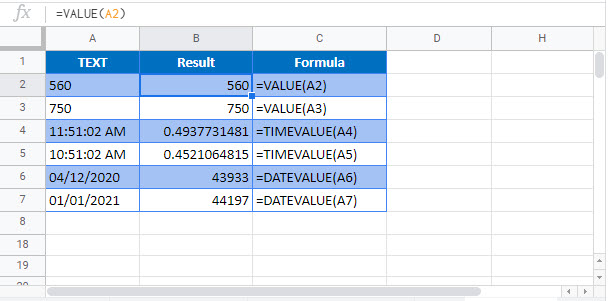
If you have a number stored as text in Excel, you can convert it to a value by using the VALUE Function.
=VALUE(B3)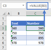
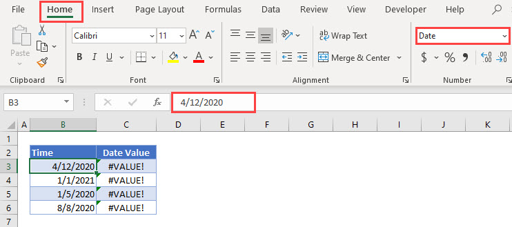
DATEVALUE Function
If you have a date stored as text in Excel, you can get the date value from it by using the DATEVALUE Function.
=DATEVALUE(B3)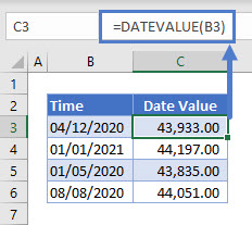
This will only work, however, if the date is stored as text.
If the date is stored as an actual date, the DATEVALUE Function will return an error.
TIMEVALUE Function
If you have time stored as text, you can use the TIMEVALUE Function to return the time value. The TIMEVALUE function will convert the text to an Excel serial number from 0 which is 12:00:00 AM to 0.999988426 which is 11:59.59 PM.
=TIMEVALUE(B3)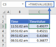
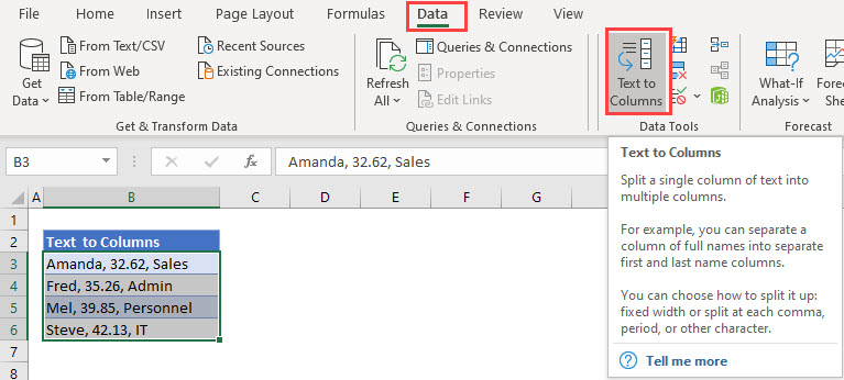
TEXT to COLUMNS
Excel has the ability to convert data stored in a text string into separate columns, using Text to Columns. If there are values within this data, it will convert the value to a number.
- Select the range to apply the formatting (ex. B3:B6)
- In the Ribbon, select Data > Text to Columns.
- Keep the option as Delimited, and click Next
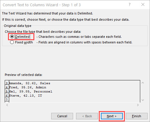
- Select Comma as the Delimiter, and make sure that the Text qualifier is set to {none}.
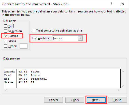
- Select cell C3 as the destination for the data. You do not need to change the Column data format as Excel will find the best match for the data.
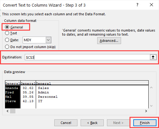
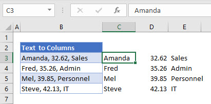
- Click Finish to view the data. If you click in cell D3, you will see that the number part of the text string has been converted to a number.
Convert Text to Number in Google Sheets
All of the examples above work the same way in google sheets.
How to Convert Text to Numbers in Excel? (Step by Step)
There are many ways we can convert text to numbers in Excel. We will see them one by one.
- Using quick convert text to numbers Excel option.
- Use a special cell formatting method.
- Using the Text to ColumnText to columns in excel is used to separate text in different columns based on some delimited or fixed width. This is done either by using a delimiter such as a comma, space or hyphen, or using fixed defined width to separate a text in the adjacent columns.read more Method.
- Using the VALUE function.
Table of contents
- How to Convert Text to Numbers in Excel? (Step by Step)
- #1 Using quick Convert Text to Numbers Excel Option
- #2 Using Paste Special Cell Formatting Method
- #3 Using the Text to Column Method
- #4 Using the VALUE Function
- Things to Remember
- Recommended Articles
You can download this Convert Text to Numbers Excel Template here – Convert Text to Numbers Excel Template
#1 Using quick Convert Text to Numbers Excel Option
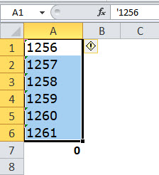
It is probably the simplest of ways in Excel. Many people use the apostrophe ( ‘ ) before entering the numbers in Excel.
Below are the steps for converting text to numbers Excel option:
- We must first select the data.

- Then, we need to click on the error handle box and select the “Convert to Number” option.

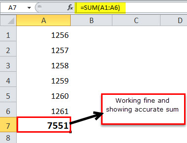
- That would instantly convert the text-formatted numbers to number format, and now the SUM function works well and shows the accurate result.


#2 Using Paste Special Cell Formatting Method
Now let us move to another way of changing the text to numbers. Here we are using the Paste Special methodPaste special in Excel allows you to paste partial aspects of the data copied. There are several ways to paste special in Excel, including right-clicking on the target cell and selecting paste special, or using a shortcut such as CTRL+ALT+V or ALT+E+S.read more. Again, consider the same data we used in the previous example.
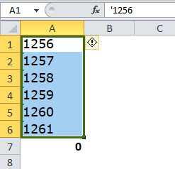
- Step 1: First, we must type the number either zero or 1 in any one cell.
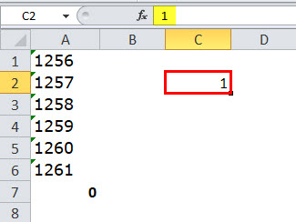
- Step 2: Now, we need to copy that number. (We have entered the number 1 in cell C2).
- Step 3: Now, we must select the numbers list.
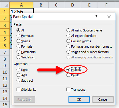
- Step 4: Now, we must press ALT + E + S (Excel shortcut keyAn Excel shortcut is a technique of performing a manual task in a quicker way.read more for the pastespecial method). That will open up the below dialog box. Select the multiply option. (We can try to divide also).
- Step 5: As a result, it would instantly convert the text to numbers, and the SUM formula is working well now.
#3 Using the Text to Column Method
It is the third method of converting text to numbers. It is a bit lengthier process than the earlier two, but it is always good to have as many alternatives as possible.
- Step 1: We must first select the data
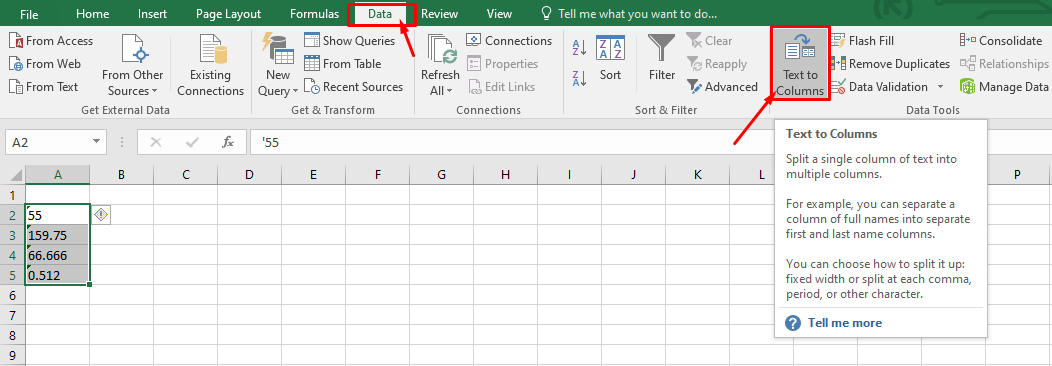
- Step 2: We need to click on the “Data” tab and the “Text to Columns” option.
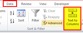
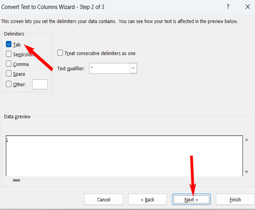
- Step 3: As a result, it will open up the below dialog box and ensure “Delimited” is selected. Click on the “Next button.”
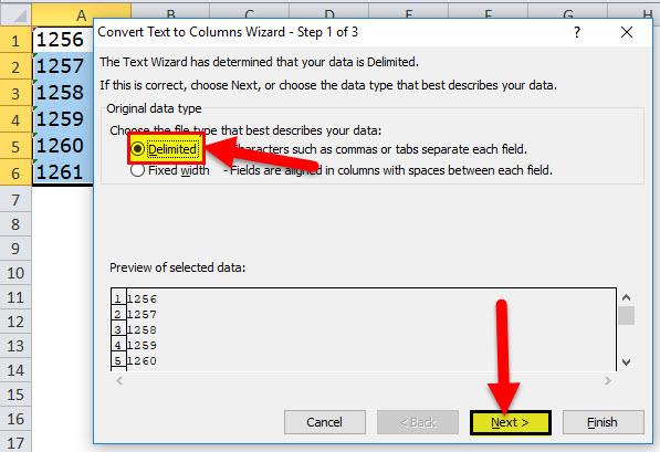
- Step 4: We must ensure the “Tab” box is checked and click on the “Next” button.
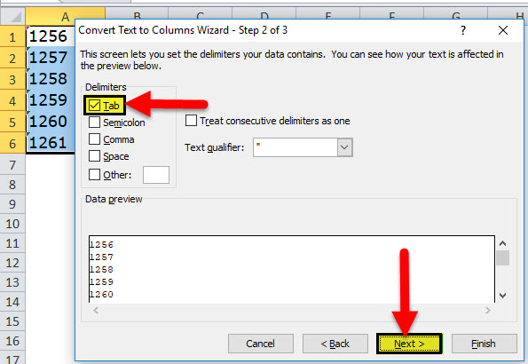
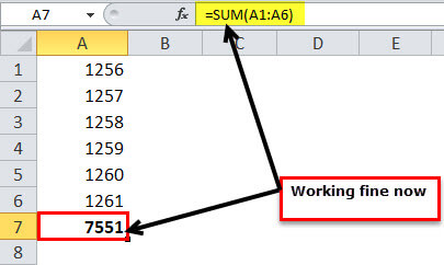
- Step 5: In the next window, we must select the “General” option, select the destination cell, and click on the “Finish” button.

- Step 6: Consequently, this would convert text to numbers, and SUM may work now.
#4 Using the VALUE Function
In addition, a formula can convert text to numbers in Excel. The VALUE function can perform the job for us. We must follow the below steps to learn how to do it.
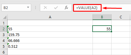
- Step 1: First, we must apply the VALUE formula in cell B1.

- Step 2: We need to drag and drop the formula into the remaining cells.

- Step 3: Then, apply the SUM formula in cell B6 to check whether it has converted or not.
Things to Remember
- If we find the green triangle button in the cell, there must be something wrong with the data.
- The VALUE function can be useful in converting the text string that represents a number to a number.
- If spacing problems exist, we nest the VALUE function with the TRIM function. For example, =Trim(Value(A1))
- The “Text to Column” can also correct dates, numbers, and time formats.
Recommended Articles
This article is a guide to Convert Text to Numbers in Excel. Here, we discuss how to convert text to numbers in Excel using 1) Error handler, 2) text to the column, 2) PasteSpecial, and 4) Value Function and Excel examples and downloadable Excel templates. You may also look at these useful functions in Excel: –
- Convert Columns to Rows in Excel
- Convert Date to Text
- Convert Numbers to Text in Excel
- Convert Excel to CSV
It is quite a frustrating situation when the numbers are formatted or stored as text in an Excel spreadsheet. Due to this, you’ll be unable to perform various Excel tasks like creating charts from values, mathematical calculations, or grouping them into arrays. But don’t worry, in this write-up, you’ll learn how to convert text to number in Excel using 6 different ways.
So, without any further ado, let’s get started…
Follow the below step-by-step methods for converting text to numerical values in MS Excel.
- Use the ‘Convert to Number’ Option
- Use Paste Special with Multiply
- Use the ‘Text to Columns’
- How to Convert the Text to Number with the VALUE Function
- Excel Convert Text To Number Using VBA
- Changing Cell Format
Way 1: Use the ‘Convert to Number’ Option to Convert Text to Number Excel
The very first way that you can try to convert text to number using the option ‘Convert to Number’. This option will eventually help you to convert the data that is been entered in the Excel with an apostrophe.
Here is how you can use this option:
- Initially, select the Excel cells that you need to convert to the number format.
- Then, you’ll see one yellow diamond exclamation symbol near the selection.
- Simply, click on a dropdown >> select the option ‘Convert to Number’.

- Now, you will be getting your text converted to the number.
Way 2: Use Paste Special with Multiply
In Microsoft Excel, Paste Special is a fabulous tool that also helps to convert text to numbers in Excel.
So, here we will use the Paste Special feature to convert the text into numbers and to perform the simple calculation.
Here is how you can do so:
- Enter the value 1, in any blank cell.
- After that select, the particular cell where you type 1 > on the Edit menu. Click Copy.
- And with the values select the cells that you need to convert to numbers.
- Next on Edit menu >> click Paste Special.

- Then under Paste Special operation >> select All >> click Multiply >> OK.

Note: If you are getting any issues while pasting your data in the Excel worksheet, check out this post.
Way 3: Use the ‘Text to Columns’
This method works best if data is arranged in a single column. The example presumes that the data is in column A and starts in row 1 ($A$1).
Follow the steps to do so:
- Choose one column of cells that holds the text.
- And on the Data menu > click Text to Columns.
- After that under Original data type > click Delimited > click Next.
- Next under Delimiters > click to choose the Tab check box > click Next.
- And under Column data format > click General.
- Then click Advanced > make any appropriate settings for the Decimal separator > Thousands separator and click OK.
- Click Finish.

And that all your text is converted to numbers.
Way 4: How to Convert Text to Number in Excel with the VALUE Function
The VALUE function is a handy way that can be used for converting the text to numbers.
Here you have to type the below command in the cell:
= VALUE (text)
- Here, text is the value that you need to convert to a numerical value.
In case, if your text contains non-numerical characters, the VALUE function returns a #VALUE! error. And it doesn’t give you the result that you want.
= VALUE (B3)
Now, the above formula can be used to convert text in the Excel cell B3 to a numerical value and then copy & paste a formula in order to convert the complete column.
Way 5: Excel Convert Text To Number Using VBA
Another very interesting way to make your Convert Text to Numerical values is by using the VBA code. It is well applicable to Excel 2003/2007 application version.
It is found that in many cases all the above-mentioned solution fails to work. Well in a such situation, using VBA works great.
The following VBA Macro code is provided on the Microsoft page to make Excel convert Text to Number.
Sub Enter_Values()
For Each xCell In Selection
xCell.Value = xCell.Value
Next xCell
End Sub
If in case the above VBA code shows an error on execution, then you need to do the following changes in coding:
For Each xCell In Selection
xCell.Value = CDec(xCell.Value)
Next xCell
Way 6: Changing Cell Format
Changing the cell format is another yet way that can assist you to convert text to number Excel successfully.
- For this, you have to right-click on the cell(s).
- Click on “Format Cells.”

- After this, choose “Number” tab >> click on “Number” on a left.
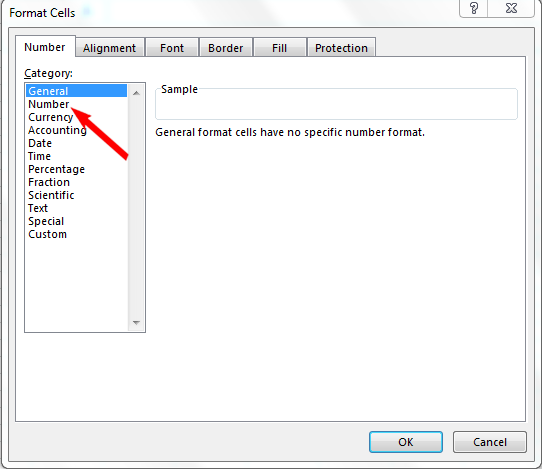
- Now, you can adjust the Decimal Places >> click “OK.”
Related FAQs:
What Is the Shortcut to Convert to Number in Excel?
The Ctrl + Alt + V is the shortcut to convert to numbers. All you need to do is to select the cells that you need to convert to numbers, then press the Ctrl + Alt + V keys simultaneously.
How Do I Convert Text to Number in Excel VLOOKUP?
By using the Value Function, you can convert the text to number in Excel VLOOKUP.
How Do I Convert Text to Number in Excel Cell?
You can convert text to number in Excel cell using the Paste Special feature, error checking, or Value Function.
Also Read: How to Convert Access To Excel File? [The Definitive Guide]
To Sum Up
Well, this is all about how to convert text to number in Excel in easy ways. I tried my level best to put together the possible steps that will help you out.
All you need to do is to follow the given steps one by one and convert text to number in MS Excel effortlessly.
Thanks for reading this post!

Priyanka is an entrepreneur & content marketing expert. She writes tech blogs and has expertise in MS Office, Excel, and other tech subjects. Her distinctive art of presenting tech information in the easy-to-understand language is very impressive. When not writing, she loves unplanned travels.