Text string function excel - Word и Excel - помощь в работе с программами

The TEXT function lets you change the way a number appears by applying formatting to it with format codes. It’s useful in situations where you want to display numbers in a more readable format, or you want to combine numbers with text or symbols.

Note: The TEXT function will convert numbers to text, which may make it difficult to reference in later calculations. It’s best to keep your original value in one cell, then use the TEXT function in another cell. Then, if you need to build other formulas, always reference the original value and not the TEXT function result.

Syntax

TEXT(value, format_text)

The TEXT function syntax has the following arguments:

Argument Name	Description
value	A numeric value that you want to be converted into text.
format_text	A text string that defines the formatting that you want to be applied to the supplied value.

Overview

In its simplest form, the TEXT function says:

=TEXT(Value you want to format, «Format code you want to apply»)

Here are some popular examples, which you can copy directly into Excel to experiment with on your own. Notice the format codes within quotation marks.

Formula	Description
=TEXT(1234.567,«$#,##0.00»)	Currency with a thousands separator and 2 decimals, like $1,234.57. Note that Excel rounds the value to 2 decimal places.
=TEXT(TODAY(),«MM/DD/YY»)	Today’s date in MM/DD/YY format, like 03/14/12
=TEXT(TODAY(),«DDDD»)	Today’s day of the week, like Monday
=TEXT(NOW(),«H:MM AM/PM»)	Current time, like 1:29 PM
=TEXT(0.285,«0.0%»)	Percentage, like 28.5%
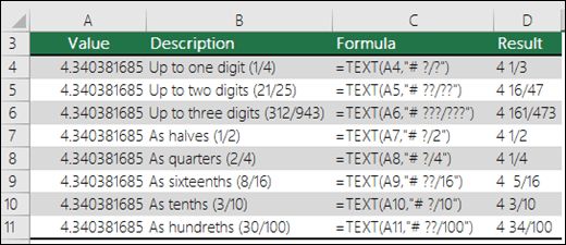
=TEXT(4.34 ,«# ?/?»)	Fraction, like 4 1/3
=TRIM(TEXT(0.34,«# ?/?»))	Fraction, like 1/3. Note this uses the TRIM function to remove the leading space with a decimal value.
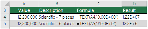
=TEXT(12200000,«0.00E+00»)	Scientific notation, like 1.22E+07
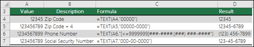
=TEXT(1234567898,«[<=9999999]###-####;(###) ###-####»)	Special (Phone number), like (123) 456-7898
=TEXT(1234,«0000000»)	Add leading zeros (0), like 0001234
=TEXT(123456,«##0° 00′ 00»»)	Custom — Latitude/Longitude

Note: Although you can use the TEXT function to change formatting, it’s not the only way. You can change the format without a formula by pressing CTRL+1 (or +1 on the Mac), then pick the format you want from the Format Cells > Number dialog.

Download our examples

You can download an example workbook with all of the TEXT function examples you’ll find in this article, plus some extras. You can follow along, or create your own TEXT function format codes.

Download Excel TEXT function examples

Other format codes that are available

You can use the Format Cells dialog to find the other available format codes:

Press Ctrl+1 (+1 on the Mac) to bring up the Format Cells dialog.
Select the format you want from the Number tab.
Select the Custom option,
The format code you want is now shown in the Type box. In this case, select everything from the Type box except the semicolon (;) and @ symbol. In the example below, we selected and copied just mm/dd/yy.
Press Ctrl+C to copy the format code, then press Cancel to dismiss the Format Cells dialog.
Now, all you need to do is press Ctrl+V to paste the format code into your TEXT formula, like: =TEXT(B2,»mm/dd/yy«). Make sure that you paste the format code within quotes («format code»), otherwise Excel will throw an error message.

Format codes by category

Following are some examples of how you can apply different number formats to your values by using the Format Cells dialog, then use the Custom option to copy those format codes to your TEXT function.

Why does Excel delete my leading 0’s?

Excel is trained to look for numbers being entered in cells, not numbers that look like text, like part numbers or SKU’s. To retain leading zeros, format the input range as Text before you paste or enter values. Select the column, or range where you’ll be putting the values, then use CTRL+1 to bring up the Format > Cells dialog and on the Number tab select Text. Now Excel will keep your leading 0’s.

If you’ve already entered data and Excel has removed your leading 0’s, you can use the TEXT function to add them back. You can reference the top cell with the values and use =TEXT(value,»00000″), where the number of 0’s in the formula represents the total number of characters you want, then copy and paste to the rest of your range.

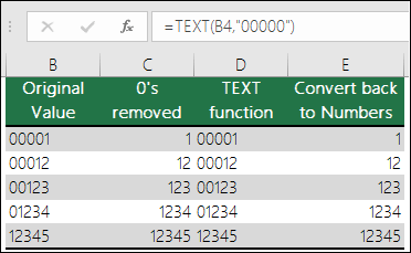
If for some reason you need to convert text values back to numbers you can multiply by 1, like =D4*1, or use the double-unary operator (—), like =—D4.

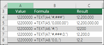
Excel separates thousands by commas if the format contains a comma (,) that is enclosed by number signs (#) or by zeros. For example, if the format string is «#,###», Excel displays the number 12200000 as 12,200,000.

A comma that follows a digit placeholder scales the number by 1,000. For example, if the format string is «#,###.0,», Excel displays the number 12200000 as 12,200.0.

Notes:

The thousands separator is dependent on your regional settings. In the US it’s a comma, but in other locales it might be a period (.).
The thousands separator is available for the number, currency and accounting formats.

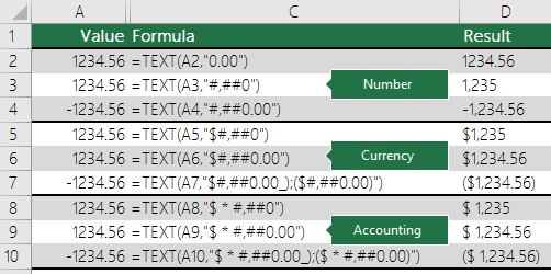
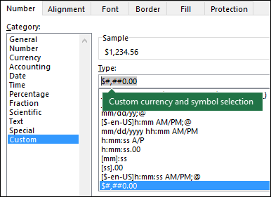
Following are examples of standard number (thousands separator and decimals only), currency and accounting formats. Currency format allows you to insert the currency symbol of your choice and aligns it next to your value, while accounting format will align the currency symbol to the left of the cell and the value to the right. Note the difference between the currency and accounting format codes below, where accounting uses an asterisk (*) to create separation between the symbol and the value.

To find the format code for a currency symbol, first press Ctrl+1 (or +1 on the Mac), select the format you want, then choose a symbol from the Symbol drop-down:

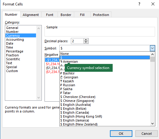
Then click Custom on the left from the Category section, and copy the format code, including the currency symbol.

Note: The TEXT function does not support color formatting, so if you copy a number format code from the Format Cells dialog that includes a color, like this: $#,##0.00_);[Red]($#,##0.00), the TEXT function will accept the format code, but it won’t display the color.

You can alter the way a date displays by using a mix of «M» for month, «D» for days, and «Y» for years.

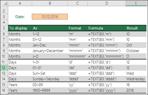
Format codes in the TEXT function aren’t case sensitive, so you can use either «M» or «m», «D» or «d», «Y» or «y».

You can alter the way time displays by using a mix of «H» for hours, «M» for minutes, or «S» for seconds, and «AM/PM» for a 12-hour clock.

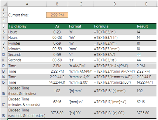
If you leave out the «AM/PM» or «A/P», then time will display based on a 24-hour clock.

Format codes in the TEXT function aren’t case sensitive, so you can use either «H» or «h», «M» or «m», «S» or «s», «AM/PM» or «am/pm».

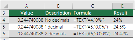
You can alter the way decimal values display with percentage (%) formats.

You can alter the way decimal values display with fraction (?/?) formats.

Scientific notation is a way of displaying numbers in terms of a decimal between 1 and 10, multiplied by a power of 10. It is often used to shorten the way that large numbers display.

Excel provides 4 special formats:

Zip Code — «00000»
Zip Code + 4 — «00000-0000»
Phone Number — «[<=9999999]###-####;(###) ###-####»
Social Security Number — «000-00-0000»

Special formats will be different depending on locale, but if there aren’t any special formats for your locale, or if these don’t meet your needs then you can create your own through the Format Cells > Custom dialog.

Common scenario

The TEXT function is rarely used by itself, and is most often used in conjunction with something else. Let’s say you want to combine text and a number value, like “Report Printed on: 03/14/12”, or “Weekly Revenue: $66,348.72”. You could type that into Excel manually, but that defeats the purpose of having Excel do it for you. Unfortunately, when you combine text and formatted numbers, like dates, times, currency, etc., Excel doesn’t know how you want to display them, so it drops the number formatting. This is where the TEXT function is invaluable, because it allows you to force Excel to format the values the way you want by using a format code, like «MM/DD/YY» for date format.

In the following example, you’ll see what happens if you try to join text and a number without using the TEXT function. In this case, we’re using the ampersand (&) to concatenate a text string, a space (» «), and a value with =A2&» «&B2.

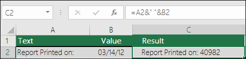
As you can see, Excel removed the formatting from the date in cell B2. In the next example, you’ll see how the TEXT function lets you apply the format you want.

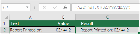
Our updated formula is:

Cell C2:=A2&» «&TEXT(B2,»mm/dd/yy») — Date format

Frequently Asked Questions

Yes, you can use the UPPER, LOWER and PROPER functions. For example, =UPPER(«hello») would return «HELLO».

Yes, but it takes a few steps. First, select the cell or cells where you want this to happen and use Ctrl+1 to bring up the Format > Cells dialog, then Alignment > Text control > check the Wrap Text option. Next, adjust your completed TEXT function to include the ASCII function CHAR(10) where you want the line break. You might need to adjust your column width depending on how the final result aligns.

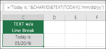
In this case, we used: =»Today is: «&CHAR(10)&TEXT(TODAY(),»mm/dd/yy»)

This is called Scientific Notation, and Excel will automatically convert numbers longer than 12 digits if a cell(s) is formatted as General, and 15 digits if a cell(s) is formatted as a Number. If you need to enter long numeric strings, but don’t want them converted, then format the cells in question as Text before you input or paste your values into Excel.

1. LEN Function

LEN function returns the count of characters in the value. In simple words, with the LEN function, you can count how many characters are there in value. You can refer to a cell or insert the value in the function directly.

Syntax

LEN(text)

Arguments

text: A string for which you want to count the characters.

Example

In the below example, we have used the LEN to count letters in a cell. “Hello, World” has 10 characters with a space between and we have got 11 in the result.

In the below example, “22-Jan-2016” has 11 characters, but LEN returns 5.

The reason behind it is that the LEN function counts the characters in the value of a cell and is not concerned with formatting.

Related: How to COUNT Words in Excel

2. FIND Function

FIND function returns a number which is the starting position of a substring in a string. In simple words, by using the find function you can find (case sensitive) a string’s starting position from another string.

Syntax

FIND(find_text,within_text,[start_num])

Arguments

find_text: The text which you want to find from another text.
within_text: The text from which you want to locate the text.
[start_num]: The number represents the starting position of the search.

Example

In the below example, we have used the FIND to locate the “:” and then with the help of MID and LEN, we have extracted the name from the cell.

3. SEARCH Function

SEARCH function returns a number which is the starting position of a substring in a string. In simple words, with the SEARCH function, you can search (non-case sensitive) for a text string’s starting position from another string.

Syntax

SEARCH(find_text,within_text,[start_num])

Arguments

find_text: A text which you want to find from another text.
within_text: A text from which you want to locate the text. You can refer to a cell, or you can input a text in your function.

Example

In the below example, we are searching for the alphabet “P” and we have specified start_num as 1 to start our search. Our formula returns 1 as the position of the text.

But, if you look at the word, we also have a “P” in the 6th position. That means the SEARCH function can only return the position of the first occurrence of a text, or if you specify the start position accordingly.

4. LEFT Function

LEFT Functions return sequential characters from a string starting from the left side (starting). In simple words, with the LEFT function, you can extract characters from a string from its left side.

Syntax

LEFT(text,num_chars)

Arguments

text: A text or number from which you want to extract characters.
[num_char]: The number of characters you want to extract.

Example

In the below example, we have extracted the first five digits from a text string using LEFT by specifying the number of characters to extract.

In the below example, we have used LEN and FIND along with the LEFT to create a formula that extracts the name from the cell.

5. RIGHT Function

The RIGHT function returns sequential characters from a string starting from the right side (ending). In simple words, with the RIGHT function, you can extract characters from a string from its left side.

Syntax

RIGHT(text,num_chars)

Arguments

text: A text or number from which you want to extract characters.
[num_char]: A number of characters you want to extract.

Example

In the below example, we have extracted 6 characters using the right function. If you know, how many characters you need to extract from the string, you can simply extract them by using a number.

Now, if you look at the below example, where we have to extract the last name from the cell, but we are not confirmed about the number of characters in the last name.

So, we are using LEN and FIND to get the name. Let me show you how we have done this.

First of all, we have used the LEN to get the length of that entire text string, then we used the FIND to get the position number of space between first and last names. And in the end, we have used both the figures to get the last name.

Arguments

value1: A cell reference, an array, or a number that is directly entered into the function.
[value2]: A cell reference, an array, or a number that is directly entered into the function.

6. MID Function

MID returns a substring from a string using a specific position and number of characters. In simple words, with MID, you can extract a substring from a string by specifying the starting character and number of characters you want to extract.

Syntax

MID(text,start_num,num_chars)

Arguments

text: A text or a number from which you want to extract characters.
start_char: A number for the position of the character from where you want to extract characters.
num_chars: The number of characters you want to extract from the start_char.

Example

In the below example, we have used different values:

From the 6th character to the next 6 characters.
From the 6th character to the next 10 characters.
We have used starting a character in negative and it has returned an error.
By using 0 for the number of characters to extract and it has returned a blank.
With a negative number for the number of characters to extract and it has returned an error.
The starting number is zero and it has returned an error.
Text string directly into the function.

7. LOWER Function

LOWER returns the string after converting all the letters in small. In simple words, it converts a text string where all the letters you have are in small letters, numbers will stay intact.

Syntax

LOWER(text)

Arguments

text: The text which you want to convert to the lowercase.

Example

In the below example, we have compared the lower case, upper case, proper case, and sentence case with each other.

A lower case text has all the letters in a small case compared to others.

8. PROPER Function

The PROPER function returns the text string into a proper case. In simple words, with a PROPER function where the first letter of the word is in capital and rest in small (proper case).

Syntax

PROPER(text)

Arguments

text: The text which you want to convert to the proper case.

Example

In the below example, we have a proper case that has the first letter in the capital case in a word and the rest of the letters are in the lower case compared to the other two cases lowercase and uppercase.

In the below example, we have used the PROPER function to streamline first name and last name into the proper case.

9. UPPER Function

The UPPER function returns the string after converting all the letters in the capital. In simple words, it converts a text string where all the letters you have are in capital form and numbers will stay intact.

Syntax

UPPER(text)

Arguments

text: The text which you want to convert into uppercase.

Example

In the below example, we have used the UPPER to convert name text to capital letters from the text in which characters are in different cases.

10. REPT Function

REPT function returns a text value several times. In simple words, with the REPT function, you can specify a text, and a number to repeat that text.

Syntax

REPT(value1, [value2], …)

Example

In the below example, we have used different type of text for repetition using REPT. It can repeat any type of text or numbers and even symbols that you specify in function and the main use of the REPT function is for creating in-cell charts.

Источник

The TEXT excel function converts a number to a text string based on the format specified by the user. This format is supplied as an argument to the TEXT function. Since the resulting outputs are text representations of numbers, they cannot be used as is in formulas. Therefore, it is recommended to retain the original numbers and create a separate row or column for the converted numbers.

For example, the formula “=TEXT(“10/2/2022″,”mmmm dd, yyyy”)” returns February 10, 2022. Exclude the beginning and ending double quotation marks while entering this formula in Excel.

The purpose of using the TEXT function in Excel is to display a number in the desired format. Since this function also helps combine numbers with other text strings, it tends to make the output more legible. The TEXT function is particularly used when the number formats of different datasets need to be made identical.

Estimated reading time: 21 minutes

What is Text Function in Excel?
- Syntax of the TEXT Function of Excel
- How to Use the TEXT Function in Excel?
  - Example #1–Prefix the Text Strings to the Newly Formatted Date Values
  - Example #2–Join the Newly Formatted Time and Date Values
  - Example #3–Extract a Mobile Number from its Scientific Notation
  - Example #4–Prefix a Text String to the Initially Formatted Monetary Value
- Date Formats of Excel
- Frequently Asked Questions
- TEXT Function in Excel Video
- Recommended Articles

Syntax of the TEXT Function of Excel

The syntax of the TEXT function of Excel is shown in the following image:

The TEXT function of Excel accepts the following arguments:

Value: This is the number to be converted to a text string. Apart from a number, a date, time or cell reference can also be supplied to the TEXT excel function. The cell reference can contain either a number or an output of another function which can be a number or date.
Format_text: This is the format to be applied to the “value” argument. It is also called the format code. It is entered within double quotation marks in the TEXT formula of Excel. For instance, “0.00,” “dd/mm/yyyy,” “hh:mm:ss,” and so on are format codes.

Both the stated arguments are mandatory.

Note 1: The format code “0.00” displays a number with two decimal places. In the format code “dd/mm/yyyy,” “dd,” “mm,” and “yyyy” are the notations for days (in two digits), months (in two digits), and years (in four digits) respectively.

Likewise, “hh,” “mm,” and “ss” are the notations for hours (in two digits), minutes (in two digits), and seconds (in two digits) respectively.

For the meaning of the different date formats, refer to the heading “date formats of Excel” given after example #4 of this article.

Note 2: The TEXT function is categorized as a Text/String function of Excel. The TEXT function is available in all versions of Excel.

How to Use the TEXT Function in Excel?

Let us consider some examples to understand the working of the TEXT function in Excel.

Example #1–Prefix the Text Strings to the Newly Formatted Date Values

The following table shows the names of five children along with the dates they were born on. The dates are currently in the format m/d/yyyy. Consider the two columns and six rows of the table as columns A and B and rows 1 to 6 of Excel.

We want to perform the following tasks:

Join the name and date of birth of row 2 by using the ampersand operator. There should not be any space between the joined values.
Convert each date to the format “dd mmm, yyyy.” Prefix the child’s name and the string “was born on” to each date.
Show the output when the date of row 2 is in the format “d mmm, yyyy.” Let the prefixes of the preceding point stay as it is.
Show the date formats “dd mmm, yyyy” (in cell C2) and “d mmm, yyyy” (in cell C6) in a single column.

Explain the outputs obtained in the second and fourth bullet points. Use the TEXT function of Excel.

Name of Kid	Date of Birth
John	12/8/2015
Patricia	1/12/2014
Ram	3/11/2016
Anita	11/11/2017
Davis	5/6/2014

The steps to perform the given tasks by using the TEXT function of Excel are listed as follows:

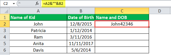
Step 1: Enter the following formula in cell C2. Exclude the beginning and ending double quotation marks while entering the given formula.

“=A2&“”&B2”

This formula (shown in the image of step 2) joins the values of cells A2 and B2 without any spaces in-between.

Note: The ampersand operator (&) helps join the values of two or more cells. It is called the concatenation operator and is used as an alternative to the CONCATENATE function of Excel. There is no limit on the number of cell values that the ampersand can join.

Step 2: Press the “Enter” key. The output appears in cell C2, as shown in the following image.

Notice that Excel has joined the values of cells A2 and B2 without any spaces in-between. However, the output is not in a readable format. The reason is that the date (12/8/2015) has been converted to a sequential number. The number 42346 represents the date December 8, 2015.

Note: A date is stored in Excel as a sequential or a serial number. This is because a serial number makes it easy to perform calculations. To view the serial number of a date, refer to the “note” preceding step 3 of example #2.

Step 3: To apply the format “dd mmm, yyyy” and insert the stated prefixes, enter the following formula in cell C2.

“=A2&” was born on “&TEXT(B2,”dd mmm, yyyy”)”

Press the “Enter” key. Then, drag the formula of cell C2 till cell C6 by using the fill handle. The outputs are displayed in the following image.

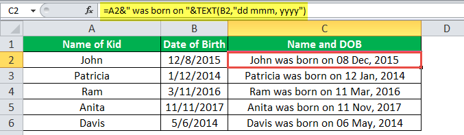
Explanation of the outputs: In column C of the preceding image, the child’s name (in column A) and the text string (was born on) have been prefixed to each date of column B. Since the date is in a suitable format, the output is readable now.

The joined values (outputs) of column C are in the form of statements that are easier to understand than the single values of columns A and B.

Notice that, to insert spaces as the separators in the output, we have inserted spaces at the relevant places in the formula of step 1. Moreover, a comma has also been inserted after the notation of months (mmm). This comma can be seen in each date of the output (in column C).

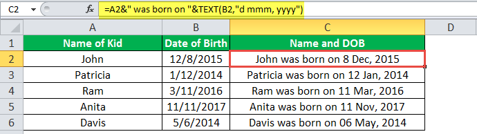
Step 4: To see the output when the date format is “d mmm, yyyy” and the prefixes are in place, enter the following formula in cell C2.

=A2&” was born on “&TEXT(B2,”d mmm, yyyy”)

Press the “Enter” key. The output appears in cell C2, as shown in the following image.

Notice that the leading zero before the date 8 Dec, 2015 (in cell C2) has disappeared. This zero was there in cell C2 of the preceding image. It has disappeared because, in the current format code, the number of days is represented by a single “d.”

A single “d” omits the leading zeros when the number of days is in a single digit.

Step 5: The outputs obtained after applying different date formats in the same column (column C) are shown in the following image.

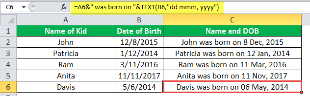
Explanation of the outputs: Notice that in the preceding image, the date of cell C2 is in the format “d mmm, yyyy” while that of cell C6 is in the format “dd mmm, yyyy.” The only difference between these two date formats is in the number of days. The leading zero is absent in cell C2 and present in cell C6.

Hence, with the TEXT function of Excel, one can have different date formats in different cells of the same column. Remember that a format code changes only the appearance of a value; it does not change the value itself. One can create a format code depending on the requirement.

Example #2–Join the Newly Formatted Time and Date Values

The following table shows the times and dates in two separate columns. Consider these columns as columns A and B of Excel. We want to perform the following tasks:

Join (concatenate) each time value with the respective date. Use the ampersand operator (&) and ensure that there is no space between the two values.
Show how to copy the formats “h:mm:ss am/pm” and “m/d/yyyy” from the “format cells” window. Convert each time to the former and date to the latter format.
Join the converted time and date values with the ampersand operator (&). Ensure that there is a space between the two values.
Show the output when the date format is not enclosed within double quotation marks.

Explain the outputs obtained in the first and third bullet points. Use the TEXT function of Excel for the given tasks.

Time	Date
7:00:00 AM	6/19/2018
7:15:00 AM	6/19/2018
7:30:00 AM	6/19/2018
7:45:00 AM	6/19/2018
8:00:00 AM	6/19/2018
8:15:00 AM	6/19/2018
8:30:00 AM	6/19/2018
8:45:00 AM	6/19/2018

The steps to perform the given tasks by using the TEXT function of Excel are listed as follows:

Step 1: Enter the following formula (without the beginning and ending double quotation marks) in cell C2.

“=A2&“”&B2”

This formula is shown in the image of step 2. It joins the values of cells A2 and B2 without a space in-between.

Step 2: Press the “Enter” key. Then, drag the formula of cell C2 till cell C9 by using the fill handle. The fill handle is displayed at the bottom-right side of cell C2.

The outputs are shown in the following image.

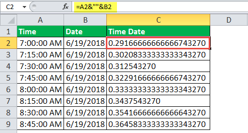
Explanation of the outputs: In column C, the number 43270 (at the end) is the same throughout the range C2:C9. This is the serial number for the date June 19, 2018. The entire decimal number preceding this serial number is the time. So, the decimal number 0.2916667 (in cell C2) represents the time 7:00:00 am.

The outputs obtained in column C of the preceding image are not readable. The reason is that Excel has converted the times (of column A) to decimal numbers and dates (of column B) to sequential numbers. Moreover, joining the decimals with sequential numbers has made the outputs more complicated.

To be able to read the output, it needs to be converted to the relevant format codes. This conversion is shown further in this example.

Note: Excel stores dates as sequential (or serial) numbers and times as decimal numbers. Excel considers a time value as a part of a day. To view the number representing the date, perform the following actions:

Select any cell of the range B2:B9.
Press the keys “Ctrl+1” together. The “format cellsFormatting cells is an important technique to master because it makes any data presentable, crisp, and in the user’s preferred format. The formatting of the cell depends upon the nature of the data present.read more” window opens.
Select “general” under “category” in the “number” tab.

The serial number can be seen under “sample.” Click “cancel” to close the “format cells” window or “Ok” to change the date to a serial number.

Likewise, the decimal number representing the time can also be seen by selecting any cell of the range A2:A9 and following actions “b” and “c” listed above.

Step 3: To convert the time and date values to a readable format, let us first copy the format codes from the “format cells” window. So, select cell C2 and press the keys “Ctrl+1” together.

The “format cells” window opens, as shown in the following image. From the “number” tab, select “custom” under “category. Excel provides a list of formats under “type.”

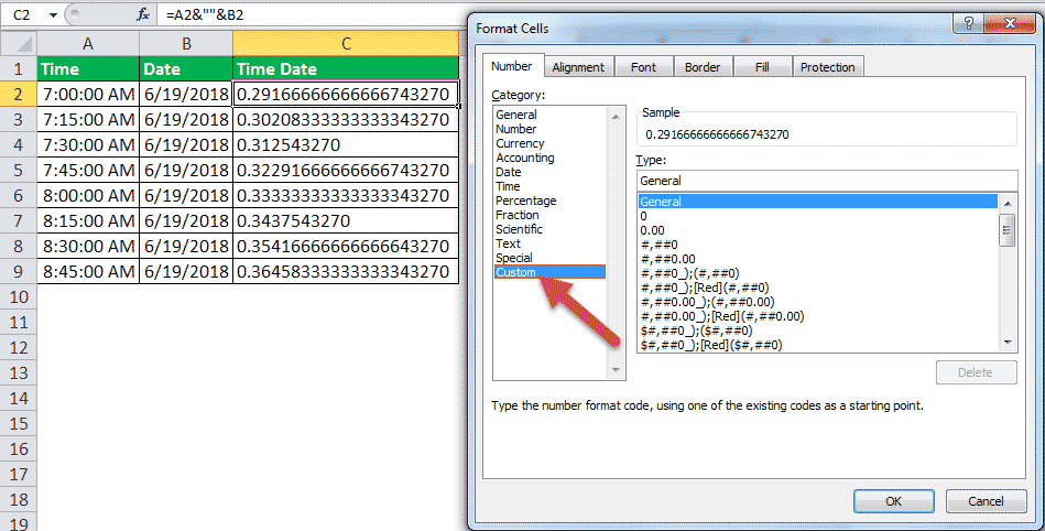
Step 4: Scroll down the list of formats given under “type.” Copy the format “h:mm:ss am/pm.” To copy, just select the format code and press the keys “Ctrl+C.”

The format code is shown in the following image. Once the format has been copied, close the “format cells” window.

Step 5: Copy the format code “m/d/yyyy” for converting the date values. This format code is also available under “type,” as shown in the following image.

Close the “format cells” window after copying the mentioned format code.

Step 6: To apply the new formats to the time and date values and join the resulting values, enter the following formula in cell C2.

“=TEXT(A2,”h:MM:SS AM/PM”)&” “&TEXT(B2,”m/d/yyyy”)”

This formula is shown in the image of step 7. If the format codes have been copied in the preceding steps, they can be pasted at the relevant places in the formula by pressing the shortcut “Ctrl+V.”

According to this formula, the time and date values of cells A2 and B2 are formatted as per the codes “h:MM:SS AM/PM” and “m/d/yyyy” respectively. The formatted (or converted) values are then joined with the ampersand operator.

Notice that in the formula, a space has also been entered within a pair of double quotation marks (like &“ ”&). This space will be inserted in the output at exactly that place where it has been entered in the formula.

Step 7: Press the “Enter” key after entering the TEXT formula. Drag the formula of cell C2 till cell C9.

The outputs are shown in the following image.

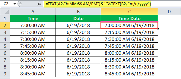
Explanation of the outputs: The time and date values of columns A and B have been converted to the relevant formats in column C. The time values display the hours (h) in a single digit, minutes (mm) in two digits, and seconds (ss) also in two digits. Since all the time values belong to the period before noon, they display “am” at the end.

Likewise, the dates display the months (m) in a single digit, days (d) in a single digit, and years (yyyy) in four digits.

Notice that there is a space between the two joined values in column C. Even though we copied the code “h:mm:ss am/pm” (in step 4) and pasted “h:MM:SS AM/PM” (in step 6), we obtained the correct outputs in column C (in step 7). This is because the format codes are not case-sensitive, implying that “mm” is treated the same as “MM.”

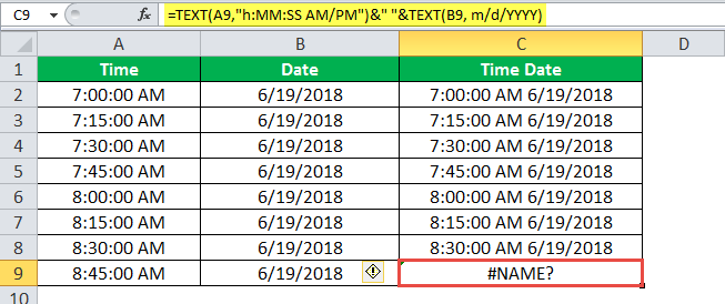
Step 8: To see what happens when the format code for date is entered without the double quotation marks, type the following formula in cell C9.

“=TEXT(A2,”h:MM:SS AM/PM”)&” “&TEXT(B2,m/d/YYYY)”

Press the “Enter” key. Excel returns the “#NAME?” error, as shown in the following image. Therefore, for the TEXT excel function to work, the format code should necessarily be enclosed within double quotation marks.

There are two images titled “image 1” and “image 2.” The following information is given:

Image 1 shows a number having eleven 9s in cell B2. When 1 is added to this number, its digits increase to 12. Excel displays the resulting 12-digit number (in cell B3) in a scientific notation.
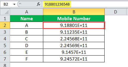
Image 2 shows the names of some people (in column A) and their random mobile numbers in a scientific notation (in column B). The formula bar shows the mobile number of person A. Each mobile number consists of twelve digits, which includes a 2-digit country code at the beginning.

Note that a scientific notationIn Excel, scientific notation is a specific style of writing numbers in scientific and exponential forms. Scientific notation compactly helps display values, allowing us to compare and use the same in calculations.read more (or scientific format) often displays very large or very small numbers in a contracted form. We want to perform the following tasks:

Display the entire 12-digit mobile number without any spaces in-between.
Separate the country code from the rest of the number with the help of a hyphen.

Use the TEXT function of Excel for the given tasks.

Image 1

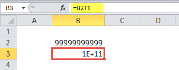
Image 2

The steps to perform the given tasks by using the TEXT function of Excel are listed as follows:

Step 1: Enter the following formula in cell D2.

“=TEXT(B2,”############”)”

This formula is shown in the formula bar of the succeeding image. Notice that there are 12 hashes in the formula, which represent the 12 digits of a mobile number.

Step 2: Press the “Enter” key. The output appears in cell D2. To obtain the outputs for the entire column D, drag the formula of cell D2 to cell D7. Use the fill handle of cell D2 (displayed at the bottom-right corner) for dragging.

The outputs of column D are shown in the succeeding image.

Note: The output is displayed (in column D) only when one enters a mobile number as an input (in column B) which is converted automatically (or manually) to a scientific format of Excel. In case, a scientific format is typed manually in column B; it cannot be converted to a mobile number of column D.

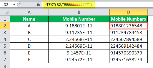
Step 3: To separate the country codes from the rest of the number by using a hyphen, enter the following formula in cell D2.

“=TEXT(B2,“##-##########”)”

Press the “Enter” key. Next, drag the formula of cell D2 till cell D7 with the help of the fill handle. The formula of cell D2 and the outputs are shown in the following image.

Notice that in the formula, the hyphen is placed exactly where it is required in the output. Since only the first two digits of each mobile number are to be separated, the hyphen is placed after two hashes of the formula.

Example #4–Prefix a Text String to the Initially Formatted Monetary Value

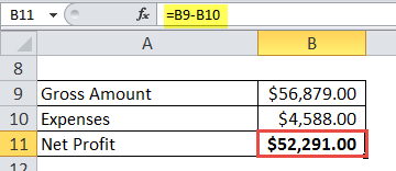
There are two images titled “image 1” and “image 2.” The following information is given:

Image 1 shows the gross profit, expenses, and net profit of an organization. All these numbers are in dollars.
Image 2 shows how the net profit has been computed. To calculate the net profit, the expenses have been subtracted from the gross profit.

We want to perform the following tasks:

Show the output when the string “the net profit is” is prefixed to the amount of net profit. Use the ampersand operator for this purpose.
Prefix the string “the net profit is” to the amount of net profit by using the ampersand. Ensure that in the output, the amount of net profit displays the dollar sign ($) and the comma at the correct places (like $52,291). Use the TEXT function of Excel for this purpose.

Explain the output obtained at the end.

Image 1

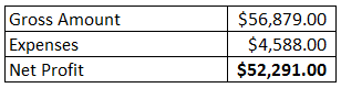
Image 2

The steps to perform the given tasks are listed as follows:

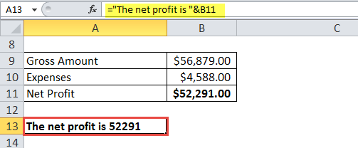
Step 1: Enter the following formula in cell A13.

“=”The net profit is “&B11”

Exclude the beginning and ending double quotation marks of the formula while entering it in Excel. This formula is shown in the image of step 2.

The given formula prefixes the string “the net profit is” to the value of cell B11. The ampersand helps join the stated string to the amount of net profit (in cell B11).

Step 2: Press the “Enter” key. The output appears in cell A13, as shown in the following image.

Notice that the dollar sign and the comma of the net profit amount (shown in cell B11) have been omitted in the output. Though the string “the net profit is” has been correctly prefixed. The spaces have also been inserted at the right places in cell A13.

Step 3: To retain the dollar sign and the comma of the amount, enter the following formula in cell A13.

“=”The net profit is ” &TEXT(B11,”$#,##0.00″)”

Press the “Enter” key. The formula and the output are shown in cell A13 of the following image.

Notice that by mistake, a space has been inserted before the ampersand in the formula. However, even then, the correct output has been obtained in cell A13.

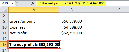
Explanation of the output: This time, the amount of net profit has been properly written (including the dollar sign and the comma) in cell A13. The reason is that the amount of net profit has been converted to the appropriate format in addition to being prefixed by a text string.

So, with the TEXT function of Excel, one can join a number with any string and, at the same time, retain the initial formatting of the number.

Date Formats of Excel

The different format codes for dates have been described as follows:

Frequently Asked Questions

1. Define the TEXT function in Excel with the help of an example.

The TEXT function in Excel helps convert a numerical value to a text string. The conversion is carried out according to the format specified by the user. Once converted, the numerical value becomes a text representation of a number.

The formula “=TEXT(“2/12/2021”,“dddd-mmmm-yyyy”)” converts the date 2/12/2021 to Thursday-December-2021. Ensure that the beginning and ending double quotation marks are excluded while entering this TEXT formula in Excel.

Note: For the working of the TEXT function of Excel, refer to the examples of this article.

2. Why is the TEXT function used in Excel?

The TEXT function is used in Excel for the following reasons:

• It helps convert a numerical value to a text string having a new format.
• It eases joining a numerical value with a text string.
• It helps retain the format of the existing numerical value after concatenation (joining).
• It makes the date or time values given in sequential or decimal numbers more readable and understandable for the users.
• It helps add the leading zeros to a number.
• It allows inserting specific characters (like +,-,(),<>,: etc.) in the output.

Note: The different characters that can be entered in the TEXT formula are the plus (+), minus (-), equal to (=), parentheses (), less than and greater than signs <>, colon (:), apostrophe (‘), curly braces {}, caret (^), forward slash (/), ampersand (&), space ( ), tilde (~), and an exclamation point (!).

The characters should be entered in the format code. These characters are displayed at exactly those places (in the output) where they have been entered in the format code.

3. How is the TEXT function used to add the leading zeros to a number in Excel?

The steps to add the leading zeros to a number are listed as follows:

a. Type “=TEXT” followed by the opening parenthesis.
b. Enter the number as the “value” argument.
c. Enter those many zeros in the format code as the number of digits required in the output.
d. Close the parenthesis and press the “Enter” key.

The leading zeros are added to the number entered in step “b.”

For instance, if the number 148 should appear as a 5-digit number, enter the formula “=TEXT(“148”,“00000”)” without the beginning and ending double quotation marks. It returns 00148.

TEXT Function in Excel Video

Recommended Articles

This has been a guide to the TEXT function of Excel. Here we discuss how to use the TEXT function in Excel along with step-by-step examples. You may also look at these useful functions of Excel–

Separate Text in ExcelThe methods used to separate text in Excel are as follows: 1) Text to Column (Delimited and Fixed Width) 2) Using Excel Formulasread more
Add Formula Text in ExcelText in Excel Formula allows us to add text values to using the CONCATENATE function or the ampersand (&) symbol.read more
INDIRECT in MS Excel
Trim FunctionThe Trim function in Excel does exactly what its name implies: it trims some part of any string. The function of this formula is to remove any space in a given string. It does not remove a single space between two words, but it does remove any other unwanted spaces.read more

Источник

Excel Text and String Functions:

Excel Functions for Finding and Replacing Text, with Examples: LEFT, RIGHT, MID, LEN, FIND, SEARCH, REPLACE, SUBSTITUTE

Related Links:

1. Excel Text and String Functions: TRIM & CLEAN.

2. Excel CODE & CHAR functions.

————————————————————————————————————————-

This section deals with the Excel Worksheet String Functions — click here for detailed explanation of Excel VBA String Functions.

LEFT Function (Worksheet / VBA)

The Excel LEFT function can be used both as a worksheet function and a VBA function. The LEFT function returns the specified number of characters in a text string, starting from the first or left-most character. Use this function to extract a sub-string from the left part of a text string. Syntax: LEFT(text_string, char_numbers). It is necessary to mention the text_string argument which is the text string from which you want to extract the specified number of characters. The char_numbers argument is optional (when using as a worksheet function), which specifies the number of characters to extract from the text string. The char_numbers value should be equal to or greater than zero; if it is greater than the length of the text string, the LEFT function will return the text string in full; if omitted, it will default to 1. While using as a VBA function, it is necessary to specify both the arguments, and if text_string contains Null, the function also returns Null.

Examples:

Cell A1 contains the text string «James Bond».

=LEFT(A1,7)

Returns «James B», which are the first 7 characters. Note that space is counted as a distinct character.

=LEFT(A1, 15)

Returns «James Bond», which are all characters in cell A1, because the number 15 specified in the function exceeds the string length of 10 characters.

=LEFT(A1)

Returns «J», a single character. Not specifying the number of characters, will default to 1.

—————————————————————————————————————————

RIGHT Function (Worksheet / VBA)

The Excel RIGHT function can be used both as a worksheet function and a VBA function. The RIGHT function returns the specified number of characters in a text string, starting from the last or right-most character. Use this function to extract a sub-string from the right part of a text string. Syntax: RIGHT(text_string, char_numbers). It is necessary to mention the text_string argument which is the text string from which you want to extract the specified number of characters. The char_numbers argument is optional (when using as a worksheet function), which specifies the number of characters to extract from the text string. The char_numbers value should be equal to or greater than zero; if it is greater than the length of the text string, the RIGHT function will return the text string in full; if omitted, it will default to 1. While using as a VBA function, it is necessary to specify both the arguments, and if text_string contains Null, the function also returns Null.

Examples:

Cell A1 contains the text string «James Bond».

=RIGHT(A1,7)

Returns «es Bond», which are the last 7 characters. Note that space is counted as a distinct character.

=RIGHT(A1, 15)

Returns «James Bond», which are all characters in cell A1, because the number 15 specified in the function exceeds the string length of 10 characters.

=RIGHT(A1)

Returns «d», a single character. Not specifying the number of characters, will default to 1.

————————————————————————————————————————

MID Function (Worksheet / VBA)

The Excel MID function can be used both as a worksheet function and a VBA function. The MID function returns the specified number of characters in a text string, starting from a specified position (ie. starting from a specified character number). Use this function to extract a sub-string from any part of a text string. Syntax: MID(text_string, start_number, char_numbers). The text_string argument is the text string from which you want to extract the specified number of characters. The start_number argument specifies the character number from which to start extracting the sub-string, the first character in a text string being start_number 1 and incrementing towards the right. The char_numbers argument specifies the number of characters to extract from the text string.

If start_number is greater than the length of the text string, an empty string (zero length) is returned; if it is less than the length of the text string but together with char_numbers (ie. start_number PLUS char_numbers) it is greater than the length of the text string, the MID function will return the text string in full from the start_number position to the end of the text string.

Using MID function as a worksheet function, if a negative value is specified for char_numbers, MID will return the #VALUE! error value; if start_number is less than 1, MID will return the #VALUE! error value. All arguments are necessary to be specified when using as a worksheet function.

Using MID function as a VBA function: The char_numbers argument is optional when used as VBA function, and if omitted the function will return the text string in full from the start_number position to the end of the text string. All other arguments are necessary to be specified when using as a vba function. If text_string contains Null, the function also returns Null.

Examples:

Cell A1 contains the text string «James Bond».

=MID(A1,2,6)

Returns «ames B». Starts from the second character ie. «a», and then specifies that 6 characters be returned starting from «a».

=MID(A1,2, 15)

Returns «ames Bond». Returns all characters starting from the second character of «a», because the specified characters number 15 plus start number 2 (ie. total of 17) exceed the string length of 10 characters.

=MID(A1, 12,2)

Returns empty text (), because the start number of 12 exceeds the string length of 10 characters.

=MID(A1,0,7)

Returns the #VALUE! error value, because the start number (ie. zero) is less than 1.

—————————————————————————————————————————

LEN Function (Worksheet / VBA)

The Excel LEN function can be used both as a worksheet function and a VBA function. The worksheet LEN function returns the number of characters in a text string. Use this function to get the length of a text string. Syntax: LEN(text_string). It is necessary to mention the text_string argument which is the text string whose length you want to get in number of characters. Note that spaces also count as characters. The worksheet LENB function returns the number of bytes used to represent the characters in a text string — counts each character as 1 byte except when a DBCS language [viz. Japanese, Chinese (Simplified), Chinese (Traditional), and Korean] is set as the default language wherein a character is counted as 2 bytes. Syntax: LENB(text_string).

While using LEN as a VBA function — Syntax: Len(text_string) or Len(variable_name) — you can use either a text string or a variable name, and the function will return a Long value representing the number of characters contained in the string or the number of bytes required to store a variable. Using the vba Len function for a variable of type variant will treat the variable as a String and return the number of characters contained in it. A text_string or variable containing Null, will also return Null. The vba Len function returns the number of characters in the string where the variable is of subtype String or Variant, and wherein the variable is of subtype numeric the function returns the number of bytes used to store the variable.

Example:

Cell A1 contains the text string «James Bond».

=LEN(A1)

Returns 10, the string length measured by its number of characters.

—————————————————————————————————————————

FIND Function (Worksheet)

The FIND function returns the starting position of a text string, which it locates from within a second text string. The starting position is the number, which is calculated beginning from the first character of that second text string. FIND is case-sensitive. Syntax: FIND(text_to_find, within_text, start_number). It is necessary to mention the first 2 arguments, while start_number argument is optional. The text_to_find argument is the text string that you want to find or locate, and it cannot contain any wildcard characters. The within_text argument is the second text string within which you want to find or search. The start_number argument specifies the character number of within_text from where you want to start the search. The first character number of within_text is 1, incrementing towards the right. Omitting the start_number argument will start your search from the first character ie. number 1. The Excel FIND function is a worksheet function. FIND is not a VBA function but can be called or used in VBA code (worksheet functions can be called from VBA using the Application or Application.Worksheet objects).

If text_to_find cannot be located in within_text, or if start_number is specified as less than 1 or greater than the length of within_text, the FIND function will return the #VALUE! error value.

If you specify text_to_find as empty text («»), the FIND function will match the character numbered start_number (or 1, if start_number is omitted) in the within_text.

Difference with SEARCH is that FIND is case sensitive and does not allow wildcard characters. If you don’t want to do a case sensitive search or use wildcard characters, you can use SEARCH.

Examples:

Cell A2 contains the text string «Australia».

=FIND(«a»,A2)

Returns 6, which is the position of the first small cap character «a» in the string.

=FIND(«A»,A2)

Returns 1, which is the position of the first large cap character «a» in the string.

=FIND(«A», A2,7)

Returns the #VALUE! error value, because text «A» is not found in the string.

=FIND(«a», A2,7)

Returns 9, which is the position of the first small cap character «a» in the string, starting from character number 7.

——————————————————————————————————————

SEARCH Function (Worksheet)

The SEARCH function returns the starting position of a text string, which it locates from within a second text string. The starting position is the number, which is calculated beginning from the first character of that second text string. SEARCH is not case-sensitive. Syntax: SEARCH(text_to_find, within_text, start_number). It is necessary to mention the first 2 arguments, while start_number argument is optional. The text_to_find argument is the text string that you want to find or locate, and it cannot contain any wildcard characters. The within_text argument is the second text string within which you want to find or search. The start_number argument specifies the character number of within_text from where you want to start the search. The first character number of within_text is 1, incrementing towards the right. Omitting the start_number argument will start your search from the first character ie. number 1. The Excel SEARCH function is a worksheet function. SEARCH is not a VBA function but can be called or used in VBA code (worksheet functions can be called from VBA using the Application or Application.Worksheet objects).

The text_to_find argument can include the wildcard characters, question mark (?) and asterisk (*). Any single character is matched using a question mark; any sequence of characters are matched using an asterisk. To find an actual question mark or asterisk, type a tilde (~) before the character.

If you specify text_to_find as empty text («»), the FIND function will match the character numbered start_number (or 1, if start_number is omitted) in the within_text.

Difference with FIND is that SEARCH is not case sensitive but allows use of wildcard characters. If you want to do a case sensitive search and not use wildcard characters, you can use FIND.

Examples:

Cell A2 contains the text string «Australia».

=SEARCH(«a»,A2)

Returns 1, which is the position of the first character «a» or «A» in the string. Note: using the FIND Function will return 6, because FIND will look for the first small cap character «a», being case-sensitive.

Cell A5 contains the text string «Daily is every day».

=SEARCH(«d?y», A5)

Returns 16, which is the starting character number of the first string which meets the criteria. This is the position of the first string that starts with «d» and ends with «y» and has only a single character inbetween.

=SEARCH(«d*y», A5)

Returns 1, which is the starting character number of the first string which meets the criteria. This is the position of the first string that starts with «d» and ends with «y» and has any number of characters inbetween. Note: The formula «=SEARCH(«d*y»,A5,2)» will return 16.

—————————————————————————————————————————

REPLACE Function (Worksheet)

The REPLACE function replaces part of a text string with a new text string, based on specified number of characters and starting from a specified position. Syntax: REPLACE(old_text, start_number, number_of_chars, new_text). It is necessary to specify all arguments. The old_text argument is the text string in which you want to replace with new text. The start_number argument is the position of the character in old_text, which you want to replace (ie. position of the first character from which replacement should start). Position is the character number, first character being number 1 & incrementing towards the right. The number_of_chars is the number of charactres which will be replaced in the old_text (with new_text). The new_text is the text string which will replace the characters in old_text.

There is also a REPLACE Function in vba, which is not being discussed here. Refer our VBA section for details.

Example:

Cell A2 contains the text string «Australia».

=REPLACE(A2, 8,2, «Asia»)

Returns «AustralAsia». Replaces 2 characters, starting with the character number 8, with «Asia».

—————————————————————————————————————————

SUBSTITUTE Function (Worksheet)

Use the SUBSTITUTE function to replace old text with new text in a text string. Substitute Function vs Replace Function: The difference is that in Substitute you replace specific text with new text while in Replace you replace any text based on its position and length within a text string. Syntax: SUBSTITUTE(text, old_text, new_text, instance_num). It is necessary to specify all arguments except instance_num. The text argument is the text string which contains the old text which you want to replace. The old_text argument is the text string which you want to replace with new text. The new_text argument is the new text which replaces the old text. The instance_num argument is a numerical value which specifies the occurrence of old text which you want to replace with new text. All occurrences of old text within the text string will be replaced with new text if you omit to specify this argument, else only the specified number of occurrences of the old text will be replaced with new text.

Examples:

Cell A2 contains the text string «Australia».

=SUBSTITUTE(A2,»ia», «Asia»)

Returns «AustralAsia». Substitutes «ia» with «Asia».

Cell A4 contains the text string «Tue, Feb 01, 2011».

=SUBSTITUTE(A4,1, 2,3)

Returns «Tue, Feb 01, 2012». Substitutes the third instance of «1» with «2».

=SUBSTITUTE(A4, 1,2)

Returns «Tue, Feb 02, 2022». Substitutes all instances of «1» with «2».

—————————————————————————————————————————

Nesting FIND within MID (Example)

Cell A3 contains the text string «James Bond Daniel Craig», and we want to replace a part of the text so as to have the new string «James Bond 007».

=MID(A3,1,FIND(«Daniel Craig», A3)-1)& «007» [Formula]

Returns the string «James Bond 007».

=FIND(«Daniel Craig», A3) -> This part of the formula returns 12, which is the position of «Daniel Craig» in the text. Deduct 1 from this number, to arrive at the position of the last character in the text before «Daniel Craig».

=MID(A3,1,FIND(«Daniel Craig», A3)-1) -> This part returns the text «James Bond «, having deleted the text «Daniel Craig» which we wish to replace. MID Function returns 11 characters (note that there is a space after James Bond) from the text string, starting from character number 1.

=MID(A3,1,FIND(«Daniel Craig», A3)-1)& «007» -> This completes the formula by adding the text «007». We have now replaced the text «Daniel Craig» with «007», to return the string «James Bond 007».

Nesting FIND within REPLACE (Example)

Cell A3 contains the string «James Bond Daniel Craig», and we want to replace a part of the text so as to have the new string «James Bond 007».

=REPLACE(A3, FIND(«Daniel Craig», A3),13, «007») [Formula]

Returns the string «James Bond 007».

=FIND(«Daniel Craig»,A3) -> This part of the formula returns 12, which is the position of «Daniel Craig» in the text.

=REPLACE(A3, FIND(«Daniel Craig»,A3), 12,»007″) -> The REPLACE Function replaces in the A3 string, starting with character number 12, and replaces 12 characters («Daniel Craig») in the old text. This completes the formula having now replaced the text «Daniel Craig» with «007», to return the string «James Bond 007».

Splitting a String into Separate Cells (Examples)

Example 1

We have used the LEFT, RIGHT, MID, LEN and FIND Functions to manipulate text, and split a string into separate cells — in the string (column A) each word is separated with a comma and a blank space, and the length of Month, Date & Year is fixed (3, 2 & 4 characters respectively) while number of characters for Day vary.

Refer Table 1 — Dates in column A have been split into separate cells, in columns C to F. We take each cell at a time, and explain how it is done.

Cell C2 contains the formula «=LEFT(A2, FIND(«,», A2)-1)», and returns the day of week as «Tuesday». FIND(«,», A2) part of the formula returns 8, which is the position of the first occurrence of the character «,» in the string. Reducing this by 1 (to 7), we use the LEFT function to extract the 7-character text (which is the day of week) appearing to the left of the character «,».

Cell D2 contains the formula «=MID(A2, FIND(«,»,A2)+2, 3)», and returns the month as «Feb». FIND(«,», A2) part of the formula returns 8, which is the position of the first occurrence of the character «,» in the string. Increasing this by 2 (to 10), we use the MID function to return the 3-character text (which is the month), starting from character number 10.

Cell E2 contains the formula «=MID(A2, FIND(«,», A2)+6, 2)», and returns the date as «01». FIND(«,», A2) part of the formula returns 8, which is the position of the first occurrence of the character «,» in the string. Increasing this by 6 (to 14), we use the MID function to return the 2-character text (which is the date), starting from character number 14.

Cell F2 contains the formula «=RIGHT(A2, 4)», and returns the year as «2011». RIGHT returns the last 4 characters in the text string, which is the corresponding year.

Example 2

The formulas have been made more complex, by using the full month name instead of the abbreviated form. Now the number of characters in the month name will vary, whereas the length of abbreviated month name was fixed (viz. 3).

Refer Table 2 — Dates in column A have been split into separate cells, in columns C to F. We take each cell at a time, and explain how it is done.

Cell C2 contains the formula «=LEFT(A2,FIND(«,», A2)-1)», and returns the day of week as «Tuesday». FIND(«,», A2) part of the formula returns 8, which is the position of the first occurrence of the character «,» in the string. Reducing this by 1 (to 7), we use the LEFT function to extract the 7-character text (which is the day of week) appearing to the left of the character «,».

Cell D2 contains the formula «=MID(A2, FIND(«,», A2)+2, LEN(A2)-9-(FIND(«,», A2)+1))», and returns the month as «February». FIND(«,»,A2) part of the formula returns 8, which is the position of the first occurrence of the character «,» in the string. Increasing this by 2 (to 10), we use the MID function to return the text (which is the month), starting from character number 10. But for this, we need to know the length of this text (ie. month name), which is determined by «LEN(A2)-9- (FIND(«,», A2)+1)». The string length of 26 [LEN(A2)] is reduced by: (i) 9, which is the number of characters after the month name ie. » 01, 2011″ (note the 2 spaces inbetween); and (ii) the formula part (FIND(«,»,A2)+1) which returns 9, which are the number of characters before start of month name ie. «Tuesday, » (note the 1 space inbetween). Therefore, length of the month name («February») is determined to be equal to: 26 minus 9 minus 9, which is 8.

Cell E2 contains the formula «=MID(A2,FIND(«,», A2, FIND(«,», A2)+1)-2, 2)», and returns the date as «01». We use the MID function to return the 2-character text (which is the date), but the starting character number is to be determined. The formula part FIND(«,»,A2,FIND(«,»,A2)+1)-2 determines this character number to start from. The formula FIND(«,»,A2)+1 returns 9, which is the next character number after the first occurrence of «,». The formula FIND(«,»,A2,FIND(«,»,A2)+1) returns 21, whihc is the position of the second occurrence of «,». Reducing this by 2 (to 19) will give us the starting character number of date, which we had set to find out. Therefore, the MID formula to find the date, will return the 2-character text date, starting from character number 19.

Cell F2 contains the formula «=RIGHT(A2, 4)», and returns the year as «2011». RIGHT returns the last 4 characters in the text string, which is the corresponding year.

Источник

Date yes Add (Subtract) Days to a Date Concatenate Dates Convert Date to Number Convert Date to Text Month Name to Number Create Date Range from Dates Day Number of Year Month Name from Date First Day of Month Add (Subtract) Weeks to a Date If Functions with Dates Max Date Number of Days Between Dates Number of Days in a Month Number of Weeks Between Dates Number of Years Between Dates Split Date & Time into Separate Cells Countdown Remaining Days Insert Dates Random Date Generator Using Dynamic Ranges — Year to Date Values Add (Subtract) Years to a Date Date Formula Examples Extract Day from Date Get Day Name from Date Count Days Left in Month / Year Count Workdays Left in Month / Year Get Last Day of Month Last Business Day of Month / Year Number of Work / Business Days in Month Weekday Abbreviations Auto Populate Dates Number of Months Between Dates Quarter from a Date Years of Service Change Date Format Compare Dates Time yes Add (Subtract) Hours to Time Add (Subtract) Minutes to Time Add (Subtract) Seconds to Time Add Up time (Total Time) Time Differences Change Time Format Convert Minutes to Hours Convert Time to Decimal Convert Time to Hours Convert Time to Minutes Convert Time to Seconds Military Time Round Time to Nearest 15 Minutes Overtime Calculator Number of Hours Between Times Convert Seconds to Minutes, Hours, or Time Count Hours Worked Time Differences Time Format — Show Minutes Seconds Text yes Add Commas to Cells Get First Word from Text Capitalize First Letter Clean & Format Phone #s Remove Extra Trailing / Leading Spaces Add Spaces to Cell Assign Number Value to Text Combine Cells with Comma Combine First and Last Names Convert Text String to Date Convert Text to Number Extract Text From Cell Get Last Word Remove Unwated Characters Extract Text Before or After Character How to Split Text String by Space, Comma, & More Remove Special Characters Remove First Characters from Left Substitute Multiple Values Switch First & Last Names w/ Commas Remove Specific Text from a Cell Extract Text Between Characters (Ex. Parenthesis) Add Leading Zeros to a Number Remove Line Breaks from Text Remove all Numbers from Text Reverse Text Remove Non-Numeric Characters Remove Last Character(s) From Right Separate First and Last Names Separate Text & Numbers Round yes Round Formulas Round Price to Nearest Dollar or Cent Round to Nearest 10, 100, or 1000 Round to Nearest 5 or .5 Round Percentages Round to Significant Figures Count yes Count Blank and Non-blank Cells Count Cells Between Two Numbers Count Cells not Equal to Count if Cells are in Range Count Times Word Appears in Cell Count Words in Cell Count Specific Characters in Column Count Total Number of Characters in Column Count Cells that Equal one of two Results Count Cells that do not Contain Count Cells that Contain Specific Text Count Unique Values in Range Countif — Multiple Criteria Count Total Number of Cells in Range Count Cells with Any Text Count Total Cells in a Table Lookup yes Two Dimensional VLOOKUP VLOOKUP Simple Example Vlookup — Multiple Matches Case Sensitive Lookup Case Sensitive VLOOKUP Sum if — VLOOKUP Case Sensitive Lookup Case Sensitive VLOOKUP Find Duplicates w/ VLOOKUP or MATCH INDEX MATCH MATCH Lookup — Return Cell Address (Not Value) Lookup Last Value in Column or Row Reverse VLOOKUP (Right to Left) Risk Score Bucket with VLOOKUP Sum with a VLOOKUP Function VLOOKUP & INDIRECT VLOOKUP Concatenate VLOOKUP Contains (Partial Match) 17 Reasons Why Your XLOOKUP is Not Working Double (Nested) XLOOKUP — Dynamic Columns IFERROR (& IFNA) XLOOKUP Lookup Min / Max Value Nested VLOOKUP Top 11 Alternatives to VLOOKUP (Updated 2022!) VLOOKUP – Dynamic Column Reference VLOOKUP – Fix #N/A Error VLOOKUP – Multiple Sheets at Once VLOOKUP & HLOOKUP Combined VLOOKUP & MATCH Combined VLOOKUP Between Worksheets or Spreadsheets VLOOKUP Duplicate Values VLOOKUP Letter Grades VLOOKUP Return Multiple Columns VLOOKUP Returns 0? Return Blank Instead VLOOKUP w/o #N/A Error XLOOKUP Multiple Sheets at Once XLOOKUP Between Worksheets or Spreadsheets XLOOKUP by Date XLOOKUP Duplicate Values XLOOKUP Multiple Criteria XLOOKUP Return Multiple Columns XLOOKUP Returns 0? Return Blank Instead XLOOKUP Text XLOOKUP with IF XLOOKUP With If Statement Misc. yes Sort Multiple Columns Use Cell Value in Formula Percentage Change Between Numbers Percentage Breakdown Rank Values Add Spaces to Cell CAGR Formula Average Time Decimal Part of Number Integer Part of a Number Compare Items in a List Dealing with NA() Errors Get Worksheet Name Wildcard Characters Hyperlink to Current Folder Compound Interest Formula Percentage Increase Create Random Groups Sort with the Small and Large Functions Non-volatile Function Alternatives Decrease a Number by a Percentage Calculate Percent Variance Profit Margin Calculator Convert Column Number to Letter Get Full Address of Named Range Insert File Name Insert Path Latitute / Longitude Functions Replace Negative Values Reverse List Range Convert State Name to Abbreviation Create Dynamic Hyperlinks Custom Sort List with Formula Data Validation — Custom Formulas Dynamic Sheet Reference (INDIRECT) Reference Cell in Another Sheet or Workbook Get Cell Value by Address Get Worksheet Name Increment Cell Reference List Sheet Names List Skipped Numbers in Sequence Return Address of Max Value in Range Search by Keywords Select Every Other (or Every nth) Row Basics yes Cell Reference Basics — A1, R1C1, 3d, etc. Add Up (Sum) Entire Column or Row Into to Dynamic Array Formulas Conversions yes Convert Time Zones Convert Celsius to Fahrenheit Convert Pounds to Kilograms Convert Time to Unix Time Convert Feet to Meters Convert Centimeters to Inches Convert Kilometers to Miles Convert Inches to Feet Convert Date to Julian Format Convert Column Letter to Number Tests yes Test if a Range Contains any Text Test if any Cell in Range is Number Test if a Cell Contains a Specific Value Test if Cell Contains Any Number Test if Cell Contains Specific Number Test if Cell is Number or Text If yes Percentile If Subtotal If Sumproduct If Large If and Small If Median If Concatentate If Max If Rank If TEXTJOIN If Sum yes Sum if — Begins With / Ends With Sum if — Month or Year to Date Sum if — By Year Sum if — Blank / Non-Blank Sum if — Horizontal Sum Count / Sum If — Cell Color INDIRECT Sum Sum If — Across Multiple Sheets Sum If — By Month Sum If — Cells Not Equal To Sum If — Not Blank Sum if — Between Values Sum If — Week Number Sum Text Sum if — By Category or Group Sum if — Cell Contains Specific Text (Wildcards) Sum if — Date Rnage Sum if — Dates Equal Sum if — Day of Week Sum if — Greater Than Sum if — Less Than Average yes Average Non-Zero Values Average If — Not Blank Average — Ignore 0 Average — Ignore Errors Math yes Multiplication Table Cube Roots nth Roots Square Numbers Square Roots Calculations yes Calculate a Ratio Calculate Age KILLLLLLL Calculate Loan Payments GPA Formula Calculate VAT Tax How to Grade Formulas Find yes Find a Number in a Column / Workbook Find Most Frequent Numbers Find Smallest n Values Find nth Occurance of Character in Text Find and Extract Number from String Find Earliest or Latest Date Based on Criteria Find First Cell with Any Value Find Last Row Find Last Row with Data Find Missing Values Find Largest n Values Most Frequent Number Conditional Formatting yes Conditional Format — Dates & Times Conditional Format — Highlight Blank Cells New Functions XLOOKUP Replaces VLOOKUP, HLOOKUP, and INDEX / MATCH Logical yes AND Checks whether all conditions are met. TRUE/FALSE IF If condition is met, do something, if not, do something else. IFERROR If result is an error then do something else. NOT Changes TRUE to FALSE and FALSE to TRUE. OR Checks whether any conditions are met. TRUE/FALSE XOR Checks whether one and only one condition is met. TRUE/FALSE Lookup & Reference yes FALSE The logical value: FALSE. TRUE The logical value: TRUE. ADDRESS Returns a cell address as text. AREAS Returns the number of areas in a reference. CHOOSE Chooses a value from a list based on it’s position number. COLUMN Returns the column number of a cell reference. COLUMNS Returns the number of columns in an array. HLOOKUP Lookup a value in the first row and return a value. HYPERLINK Creates a clickable link. INDEX Returns a value based on it’s column and row numbers. INDIRECT Creates a cell reference from text. LOOKUP Looks up values either horizontally or vertically. MATCH Searches for a value in a list and returns its position. OFFSET Creates a reference offset from a starting point. ROW Returns the row number of a cell reference. ROWS Returns the number of rows in an array. TRANSPOSE Flips the oriention of a range of cells. VLOOKUP Lookup a value in the first column and return a value. Date & Time yes DATE Returns a date from year, month, and day. DATEDIF Number of days, months or years between two dates. DATEVALUE Converts a date stored as text into a valid date DAY Returns the day as a number (1-31). DAYS Returns the number of days between two dates. DAYS360 Returns days between 2 dates in a 360 day year. EDATE Returns a date, n months away from a start date. EOMONTH Returns the last day of the month, n months away date. HOUR Returns the hour as a number (0-23). MINUTE Returns the minute as a number (0-59). MONTH Returns the month as a number (1-12). NETWORKDAYS Number of working days between 2 dates. NETWORKDAYS.INTL Working days between 2 dates, custom weekends. NOW Returns the current date and time. SECOND Returns the second as a number (0-59) TIME Returns the time from a hour, minute, and second. TIMEVALUE Converts a time stored as text into a valid time. TODAY Returns the current date. WEEKDAY Returns the day of the week as a number (1-7). WEEKNUM Returns the week number in a year (1-52). WORKDAY The date n working days from a date. WORKDAY.INTL The date n working days from a date, custom weekends. YEAR Returns the year. YEARFRAC Returns the fraction of a year between 2 dates. Engineering yes CONVERT Convert number from one unit to another. Financial yes FV Calculates the future value. PV Calculates the present value. NPER Calculates the total number of payment periods. PMT Calculates the payment amount. RATE Calculates the interest Rate. NPV Calculates the net present value. IRR The internal rate of return for a set of periodic CFs. XIRR The internal rate of return for a set of non-periodic CFs. PRICE Calculates the price of a bond. YIELD Calculates the bond yield. INTRATE The interest rate of a fully invested security. Information yes CELL Returns information about a cell. ERROR.TYPE Returns a value representing the cell error. ISBLANK Test if cell is blank. TRUE/FALSE ISERR Test if cell value is an error, ignores #N/A. TRUE/FALSE ISERROR Test if cell value is an error. TRUE/FALSE ISEVEN Test if cell value is even. TRUE/FALSE ISFORMULA Test if cell is a formula. TRUE/FALSE ISLOGICAL Test if cell is logical (TRUE or FALSE). TRUE/FALSE ISNA Test if cell value is #N/A. TRUE/FALSE ISNONTEXT Test if cell is not text (blank cells are not text). TRUE/FALSE ISNUMBER Test if cell is a number. TRUE/FALSE ISODD Test if cell value is odd. TRUE/FALSE ISREF Test if cell value is a reference. TRUE/FALSE ISTEXT Test if cell is text. TRUE/FALSE N Converts a value to a number. NA Returns the error: #N/A. TYPE Returns the type of value in a cell. Math yes ABS Calculates the absolute value of a number. AGGREGATE Define and perform calculations for a database or a list. CEILING Rounds a number up, to the nearest specified multiple. COS Returns the cosine of an angle. DEGREES Converts radians to degrees. DSUM Sums database records that meet certain criteria. EVEN Rounds to the nearest even integer. EXP Calculates the exponential value for a given number. FACT Returns the factorial. FLOOR Rounds a number down, to the nearest specified multiple. GCD Returns the greatest common divisor. INT Rounds a number down to the nearest integer. LCM Returns the least common multiple. LN Returns the natural logarithm of a number. LOG Returns the logarithm of a number to a specified base. LOG10 Returns the base-10 logarithm of a number. MOD Returns the remainder after dividing. MROUND Rounds a number to a specified multiple. ODD Rounds to the nearest odd integer. PI The value of PI. POWER Calculates a number raised to a power. PRODUCT Multiplies an array of numbers. QUOTIENT Returns the integer result of division. RADIANS Converts an angle into radians. RAND Calculates a random number between 0 and 1. RANDBETWEEN Calculates a random number between two numbers. ROUND Rounds a number to a specified number of digits. ROUNDDOWN Rounds a number down (towards zero). ROUNDUP Rounds a number up (away from zero). SIGN Returns the sign of a number. SIN Returns the sine of an angle. SQRT Calculates the square root of a number. SUBTOTAL Returns a summary statistic for a series of data. SUM Adds numbers together. SUMIF Sums numbers that meet a criteria. SUMIFS Sums numbers that meet multiple criteria. SUMPRODUCT Multiplies arrays of numbers and sums the resultant array. TAN Returns the tangent of an angle. TRUNC Truncates a number to a specific number of digits. Stats yes AVERAGE Averages numbers. AVERAGEA Averages numbers. Includes text & FALSE =0, TRUE =1. AVERAGEIF Averages numbers that meet a criteria. AVERAGEIFS Averages numbers that meet multiple criteria. CORREL Calculates the correlation of two series. COUNT Counts cells that contain a number. COUNTA Count cells that are non-blank. COUNTBLANK Counts cells that are blank. COUNTIF Counts cells that meet a criteria. COUNTIFS Counts cells that meet multiple criteria. FORECAST Predict future y-values from linear trend line. FREQUENCY Counts values that fall within specified ranges. GROWTH Calculates Y values based on exponential growth. INTERCEPT Calculates the Y intercept for a best-fit line. LARGE Returns the kth largest value. LINEST Returns statistics about a trendline. MAX Returns the largest number. MEDIAN Returns the median number. MIN Returns the smallest number. MODE Returns the most common number. PERCENTILE Returns the kth percentile. PERCENTILE.INC Returns the kth percentile. Where k is inclusive. PERCENTILE.EXC Returns the kth percentile. Where k is exclusive. QUARTILE Returns the specified quartile value. QUARTILE.INC Returns the specified quartile value. Inclusive. QUARTILE.EXC Returns the specified quartile value. Exclusive. RANK Rank of a number within a series. RANK.AVG Rank of a number within a series. Averages. RANK.EQ Rank of a number within a series. Top Rank. SLOPE Calculates the slope from linear regression. SMALL Returns the kth smallest value. STDEV Calculates the standard deviation. STDEV.P Calculates the SD of an entire population. STDEV.S Calculates the SD of a sample. STDEVP Calculates the SD of an entire population TREND Calculates Y values based on a trendline. Text yes CHAR Returns a character specified by a code. CLEAN Removes all non-printable characters. CODE Returns the numeric code for a character. CONCATENATE Combines text together. DOLLAR Converts a number to text in currency format. EXACT Test if cells are exactly equal. Case-sensitive. TRUE/FALSE FIND Locates position of text within a cell.Case-sensitive. LEFT Truncates text a number of characters from the left. LEN Counts number of characters in text. LOWER Converts text to lower case. MID Extracts text from the middle of a cell. PROPER Converts text to proper case. REPLACE Replaces text based on it’s location. REPT Repeats text a number of times. RIGHT Truncates text a number of characters from the right. SEARCH Locates position of text within a cell.Not Case-sensitive. SUBSTITUTE Finds and replaces text. Case-sensitive. TEXT Converts a value into text with a specific number format. TRIM Removes all extra spaces from text. UPPER Converts text to upper case. VALUE Converts a number stored as text into a number.

Источник

The TEXT function in Excel converts numeric values to a text string. While you’ll mostly be fiddling with numbers on an Excel sheet, you may often need to convert a few values into text. The TEXT function is available in all versions of Excel starting from Excel 2003.

Syntax

The syntax of the TEXT function is as follows:

=TEXT(value, format_text)

Arguments:

‘value’ – This is a required argument where you input the numeric value you want to convert to a text string. The supplied value can be a number, date, or a cell reference that contains a number, date, or an output from another formula that’s a number or date.
‘format_text’ – This is a required argument where you prescribe a format for the output using a format code. You can use any formatting code that Excel recognizes.

Format Codes for TEXT function

Here is a list of the most commonly used format codes that can be used with the TEXT function:

Code	Description	Example
#	Placeholder that displays significant digits.	#.## – displays up to 2 decimal places. This means if the value fed to the function is 1.755 the result will be 1.76
0	Placeholder that displays insignificant zeros.	#.000 – always displays 3 decimal places. This means if the value fed to the function is 1.75 the result will be 1.750
?	Placeholder that leaves a space for insignificant zeros but doesn’t display them. Used for presenting aligned decimals.	#.??? – displays a maximum of 3 decimal places and aligns the decimal points in the column.
.	Decimal point	–
,	Thousands separator	###,###.## – displays a thousands separator with 2 decimal places. This means if the value fed to the function is 175000, it will display as 175,000.00
d	Day of Week or Month	d – one or two-digit number representing the day of the month without a leading zero ranging from 1 to 31 dd – two-digit number representing the day of the month with a leading zero ranging from 01 to 31 ddd – three-letter abbreviation for the day of the week (Mon to Sun) dddd – full name of the day of the week (Monday to Sunday)
m	Month of the Year	m – one or two-digit number representing the month of the year without a leading zero ranging from 1 to 12 mm – two-digit number representing the month of the year with a leading zero ranging from 01 to 12 mmm – three-letter abbreviation for the month of the year (Jan to Dec) mmmm – full name of the month of the year (January to December)
y	Year	yy – two-digit number representing the last two digits of the year (e.g. 08 meaning 2008 or 20 meaning 2020) yyyy – four-digit number representing the year (e.g. 2008, 2020)
h	Hour	h – one or two-digit number representing the hour component without a leading zero (1 to 24) hh – two-digit number representing the hour component with a leading zero (01 to 24)
m	Minute (when used as part of time)	m – one or two-digit number representing the minute component without a leading zero (1 to 60) mm – two-digit number representing the minute component with a leading zero (01 to 60)
s	Second	s – one or two-digit number representing the second component without a leading zero (1 to 60) ss – two-digit number representing the second component with a leading zero (01 to 60)
AM/PM	Represents the time in 12-hour clock format, followed by «AM» or «PM»	–

Apart from the above codes if you want to display specific characters in your output, you can enter them right into the format code and they will be displayed exactly the way they have been entered. Following are the characters you can input:

Character	Description
+	Plus
–	Minus
()	Left/right parenthesis
{}	Curly brackets
<>	Less than/greater than
:	Colon
^	Caret
‘	Apostrophe
~	Tilde
/	Forward slash
!	Exclamation mark
&	Ampersand
=	Equal to
	Space

Important Characteristics of the TEXT function

The TEXT function doesn’t convert numbers to words, just text strings. For instance, if you convert 10,000 using the TEXT function, Excel will then recognize it as a text string and not a numeric value, but the function can’t convert it to the words «Ten Thousand.»
You’ll need to specify a format for the converted text.
If you enter the format code incorrectly, you’ll receive a #NAME? error.
Once you convert a numeric value using the TEXT function, you can’t manipulate it in your workbook calculations.

Examples

Let’s try to see some examples of the TEXT function.

Example 1 – Plain Vanilla Formula for the TEXT Function

Let’s use the formula on a simple, Excel-recognized date just to look at how the TEXT function works. We’ll supply a date to the function and try to format it as a «dd.mm.yyyy» text string. Here’s the formula that will help you accomplish this:

=TEXT("12/25/2000","dd.mm.yyy")

Notice how even though the original date is in the mm/dd/yyyy format, you can use the TEXT function to not only convert this date into a text string but also display it in the dd.mm.yyyy format. If you’re aiming for a more sophisticated output, you do have the option to make your date look more textual and less numeric. You’d just need to use a different format code, like so:

=TEXT("12/25/2000","mmmm d, yyyy")

This gives you a neater output. You can, of course, obtain a lot of different outputs you offer by using the relevant format code.

Alright, that takes care of the bare-bones formula, let’s do some other cool things using the TEXT function

Example 2 – Basic Arithmetic and Concatenation with the TEXT Function

Before we get to the actual example, let’s take a moment to see what you’re going to learn here.

TEXT function allows us to perform basic arithmetic operations with the values that are supplied to it. Instead of directly supplying a value or cell reference, you can do some arithmetic within the argument.

And in addition to this, it also supports concatenation. Concatenation relates to combining the output of the TEXT function with another text string to make the output more contextual.

Okay, so consider that you’re at your job or business desk looking at a price list. You plan on offering discounts to customers, and each product has a different discount rate. You have a list of customers that have gotten in touch with you to claim their discount, and you need to compute their final price. You plan on using the mail merge feature in MS Word and send the customers a letter about their final price.

You’ve got the original price and the discount rate for Product A listed on your sheet. In the third column labeled MESSAGE, you want the final message that you’ll send to your customers. Here’s the formula you can use to do this:

="The discounted price is "&TEXT(A2*(1-B2),"$###,###.00")

There are a couple of things going on in this formula. The first portion of the formula is just a plain text string; no formulas in the first portion. The text string is concatenated using the ampersand (&), which means the text string will be connected with the text string that the second portion of the formula returns.

Let’s switch over to the second part of the formula, where we’ve used the TEXT function. The first argument, this time, is an arithmetic operation instead of a numeric value supplied directly or as a cell reference. The calculation is essentially for the discounted price. The second portion of the formula is again just a format code, which will format the output in a way that it has a comma separator after every three digits, and with two decimal values at the end.

The final output gives you a ready to import text string that you can use in your mail merge letters or envelopes for marketing. Who knew Excel could contribute to your marketing efforts, eh?

Alright, let’s flex our muscles a little more.

Example 3 – Add Padding Zeros to Numbers with the TEXT Function

This is one of the most common use-cases of the TEXT function. When you have a list of numbers with a varying number of digits, and you want a nice list where all numbers that have less than a certain number of digits have 0s at the beginning. Let’s make this a little clearer with an example.

Say you’ve got some numbers piled up in your worksheet. The smallest number is 2 digits, while the largest number is 7 digits. You want to give it a tidy look so all numbers will essentially be 7 digits. Here’s the formula you could use:

=TEXT(A2,"0000000")

You’re effectively just giving the cells a format where any number with less than 7 digits will have 0s as a prefix for padding. Note that once you’ve applied the TEXT function to these numbers, they’re no longer numbers that you can manipulate on your spreadsheet, they’re just text strings.

You can now feed your secret OCD just right.

Example 4 – Get Day Name from Week

You’ve been told that some employees have been slacking off and you intend to set things straight with them. You have a software that records attendance from employees, but unfortunately, the software also includes the weekends into the list of days when employees wouldn’t have punched their cards in.

You now have a list of dates on which your employees didn’t show up, but you need to weed out the holidays from working days. Manually, this could take you about a million years. Thanks to Excel, we’ve got a way to accomplish this within a couple of seconds.

Assume that you give Saturdays and Sundays off. Then, you’ll need to identify the dates that fall on a Saturday or Sunday so you don’t end up nagging the employee for no good reason. Once you’ve got the Saturdays and Sundays out of the list, you know which workdays your employees didn’t show up on.

Perhaps, you could call upon the TEXT function for some help with the following formula:

=TEXT(A2,"dddd")

Since the format has been set to «dddd» it shows the full name of the day. You could also choose to format the output as «ddd» to display the output as Mon, Tue, Wed, etc.

As you’d have noticed, all we’re doing with this formula is just changing the dates into text and formatting it such that the final output displays the day component of the date. If you have a fairly large list, you can also give your output some conditional formatting so you can eyeball employees that have taken excessive holidays.

There’s one more thing you can use the same formula for, but you’ll need to tweak it just a tad. Let’s talk about that in the next example.

Recommended Reading: Get Day of Week From Date In Excel

Example 5 – Get Month Name from Week

Say you’re now keen on analyzing which month witnessed the highest leaves. Maybe, the absenteeism was a cause of flu season. To understand this, you need to see which month the dates where employees didn’t show up fall in.

To accomplish this, you can use a slight variation of the previous formula. If you hadn’t guessed it already, the formula is:

=TEXT(A2,"mmmm")

This is the same formula we used in the previous example, but this time, the final output has been formatted to show the name of the month instead of the day. Note that all output cells are now formatted as text strings and you cannot use them for manipulation on your worksheet.

Like we discussed in the previous example, you can also give the output in this example different formatting if you so choose. For instance, if you want to display the three-word abbreviation of a month (like Jan, Feb, Mar, etc.) instead of the full name, you could use the «mmm» format.

All set? Alright, time to play with some numbers.

Example 6 – Convert Numbers to Phone Number Format

Have you had to skim through what looks like a gazillion phone numbers, all of which have a country code as a prefix? It makes you dizzy looking through the digit-dense list, but a little formatting could make things a lot easier for you.

Say you’ve got some cell phone numbers listed on your spreadsheet. They’re all 10-digit numbers but have a country code in front of them. You want to separate the country code so it’s easier to see which country the number belongs to.

Remember, the TEXT function gives you a ton of ammunition for custom formatting the output. Therefore, it can be a great tool to tidy up your spreadsheet regardless of what data you have in your cells. Here’s the formula we’ll use to clean up the list of phone numbers:

=TEXT(A2,"(##) ##### #####")

You now have all country codes in brackets, well organized, and easy to read.

Also, remember those characters we said you could add to the format and they’ll appear as they are entered in the formula? We’ve used parentheses in this formula and notice how they appear as-is in the final output. If you prefer, you could even add dashes instead of spaces between the numbers, and it would work just fine.

Pretty cool, huh?

Example 7 – Concatenate a Date with Text Using the TEXT Function

Say you want to create an output where there’s a text string concatenated with the DATE function to display something like, «Today is January 1, 2001». Go ahead and give it a try. If you don’t know the formula, here you go:

= "Today is " &DATE(2001,1,1)

See the problem?

This formula gives you an output where the DATE is displayed as a serial number. Technically, Excel is doing everything that it’s supposed to. For Excel, a date is a serial number and is displayed as such unless otherwise formatted.

As we discussed previously, the TEXT function carries plenty of power when it comes to formatting the output. So, we’ll add the TEXT function to the mix just to change the format of the output.

Note that the Excel function is doing nothing except for formatting in the following formula:

="Today is "&TEXT(DATE(2000,12,25),"mmmm d, yyyy")

Notice that all that’s different in this formula is that we’ve nested the DATE function inside the TEXT function so we can format the serial number as «mmmm d, yyyy». The DATE function relays the serial number to the TEXT function, which then converts it into the prescribed format.

Easy-peasy, isn’t it?

Alright, that’s a wrap for the TEXT function. TEXT function, quite literally, is one of the most versatile functions when it comes to formatting. It can help you organize and tidy up almost any data set you have based on your preferred output format. So, once you’ve championed all these formulas (they’re quite easy, aren’t they?), we’ll have the next tutorial ready for you to get your hands dirty with. Meanwhile, stay curious!

Источник

This Excel tutorial explains how to use the Excel TEXT function with syntax and examples.

Description

The Microsoft Excel TEXT function returns a value converted to text with a specified format.

The TEXT function is a built-in function in Excel that is categorized as a String/Text Function. It can be used as a worksheet function (WS) in Excel. As a worksheet function, the TEXT function can be entered as part of a formula in a cell of a worksheet.

Syntax

The syntax for the TEXT function in Microsoft Excel is:

TEXT( value, format )

Parameters or Arguments

value: The value to convert to text.
format: The format used to display the result.

Returns

The TEXT function returns a string/text value.

Applies To

Excel for Office 365, Excel 2019, Excel 2016, Excel 2013, Excel 2011 for Mac, Excel 2010, Excel 2007, Excel 2003, Excel XP, Excel 2000

Type of Function

Worksheet function (WS)

Example (as Worksheet Function)

Let’s look at some Excel TEXT function examples and explore how to use the TEXT function as a worksheet function in Microsoft Excel:

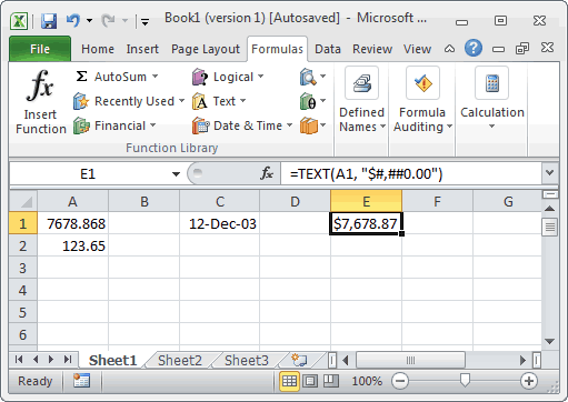
Based on the Excel spreadsheet above, the following TEXT examples would return:

=TEXT(A1, "$#,##0.00")
Result: "$7,678.87"

=TEXT(A1, "0")
Result: "7679"

=TEXT(A2, "0.0")
Result: "123.7"

=TEXT(1277, "#,##0")
Result: "1,277"

=TEXT(C1, "yyyy/mm/dd")
Result: "2003/12/12"

=TEXT(C1, "mmm dd, yyyy")
Result: "Dec 12, 2003"

Источник

Excel has many functions to offer when it comes to manipulating text strings.

Join Strings

To join strings, use the & operator.

Note: instead of using the & operator, use the CONCATENATE function in Excel.

Left

To extract the leftmost characters from a string, use the LEFT function.

Right

To extract the rightmost characters from a string, use the RIGHT function.

Mid

To extract a substring, starting in the middle of a string, use the MID function.

Note: started at position 5 (p) with length 3.

Len

To get the length of a string, use the LEN function.

Note: space (position included!

Find

To find the position of a substring in a string, use the FIND function.

Note: string «am» found at position 3. Visit our page about the FIND function for more examples.

Substitute

To replace existing text with new text in a string, use the SUBSTITUTE function.

Источник

Overview

Download our examples

Other format codes that are available

Format codes by category

Common scenario

Frequently Asked Questions

See Also

1. LEN Function

Syntax

Arguments

Example

2. FIND Function

Syntax

Arguments

Example

3. SEARCH Function

Syntax

Arguments

Example

4. LEFT Function

Syntax

Arguments

Example

5. RIGHT Function

Syntax

Arguments

Example

Arguments

6. MID Function

Syntax

Arguments

Example

7. LOWER Function

Syntax

Arguments

Example

8. PROPER Function

Syntax

Arguments

Example

9. UPPER Function

Syntax

Arguments

Example

10. REPT Function

Syntax

Example

Table of contents

Syntax of the TEXT Function of Excel

How to Use the TEXT Function in Excel?

Example #1–Prefix the Text Strings to the Newly Formatted Date Values

Example #2–Join the Newly Formatted Time and Date Values

Example #4–Prefix a Text String to the Initially Formatted Monetary Value

Date Formats of Excel

Frequently Asked Questions

TEXT Function in Excel Video

Recommended Articles

Syntax

Format Codes for TEXT function

Important Characteristics of the TEXT function

Examples

Example 1 – Plain Vanilla Formula for the TEXT Function

Example 2 – Basic Arithmetic and Concatenation with the TEXT Function

Example 3 – Add Padding Zeros to Numbers with the TEXT Function

Example 4 – Get Day Name from Week

Example 5 – Get Month Name from Week

Example 6 – Convert Numbers to Phone Number Format

Example 7 – Concatenate a Date with Text Using the TEXT Function

Description

Syntax

Parameters or Arguments

Returns

Applies To

Type of Function

Example (as Worksheet Function)

Join Strings

Left

Right

Mid

Len