
Create a Spreadsheet in Excel (Table of Content)
- Introduction to Create Spreadsheet in Excel
- How to Create a Spreadsheet in Excel?
Introduction to Create Spreadsheet in Excel
A spreadsheet is a grid-based file designed to manage or perform any calculation on personal or business data. It is the best choice for users because it has 400+ functions and features such as pivot, coloring, graph, chart, and conditional formatting. It is accessible in both Office 365 and MS Office. Office 365 is a cloud-based application, whereas MS Office is an on-premises solution.
The workbook is the Excel lingo for ‘spreadsheet.’ MS Excel uses this term to emphasize that a single workbook can contain multiple worksheets, each with its own data grid, chart, or graph.
How to Create a Spreadsheet in Excel?
Here are a few examples of creating different types of spreadsheets in Excel with the key features of the created spreadsheets.
You can download this Create Spreadsheet Excel Template here – Create Spreadsheet Excel Template
Example #1 – How to Create Spreadsheet in Excel?
Step 1: Open MS Excel.
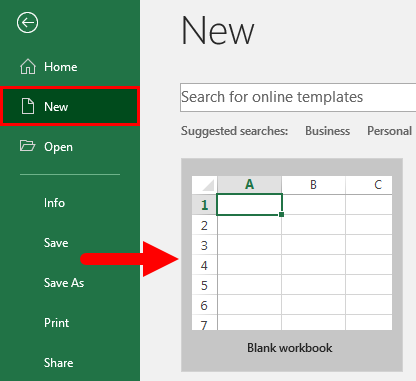
Step 2: Go to Menu and select New >> Click on the Blank workbook to create a simple worksheet.
OR – Press Ctrl + N: To create a new spreadsheet.
Step 3: By default, Sheet 1 will be created as a worksheet in the spreadsheet. The name of the spreadsheet will be given as Book 1 if you are opening it for the first time.
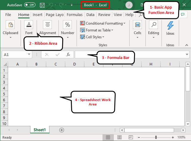
Key Features of the Created Spreadsheet:
- Basic App Functions Area: There is a green banner that contains all types of actions to perform on the worksheet, like – save the file, back or front step move, new, undo, redo, and many more.
- Ribbon Area: This is a gray area just below the basic app functions area called Ribbon. It contains data manipulation, a data visualizing toolbar, page layout tools, and many more.
- Spreadsheet Work Area: By default, a grid contains alphabetic columns like A, B, C, …, Z, ZA…, ZZ, ZZA… and rows as numbers like 1,2 3, …. 100, 101, and… so on. Each rectangle box in the spreadsheet is called a cell, like the one selected in the above image (cell A1). It is a cell where the user can perform their calculation for personal or business data.
- Formula Bar: It shows the data in the selected cell; if it contains any formula, it will show here. Like the above area, a search bar is available in the top right corner, and a sheet tab is available on the downside of the worksheet. A user can change the name of the sheet name.
Once you create an Excel Spreadsheet, you can convert it to a universally accepted format like PDF. For convenience, some useful Excel to PDF converters converts Excel to PDF files for free while maintaining the original formatting.
Example #2 – How to Create a Simple Budget Spreadsheet in Excel?
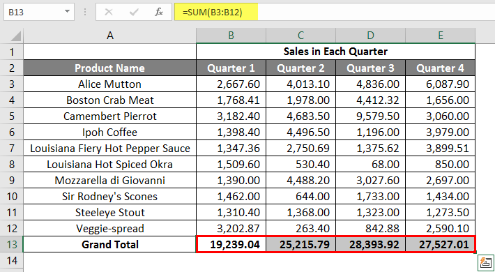
Suppose a user wishes to design a spreadsheet for budget calculation. For 2018, he has a few products and their quarterly sales. He now wants to present his client with this budget.
Let’s see how we can do this with the help of the spreadsheet.
Step 1: Open MS Excel.
Step 2: Go to Menu and select New >> Click on the Blank workbook to create a simple worksheet.
OR – Press Ctrl + N: To create a new spreadsheet.

Step 3: Go to the spreadsheet work area, sheet 1.
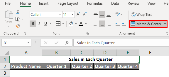
Step 4: Now create headers for Sales in each quarter in the first row by merging cells from B1 to E1. In row 2, give the product name and each quarter’s name.
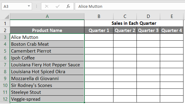
Step 5: Write down all product names in column A.
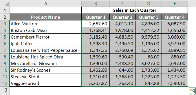
Step 6: Provide the sales data for each quarter before every product.
Step 7: In the next row, put one header for Grand Total and calculate each quarter’s total sales.
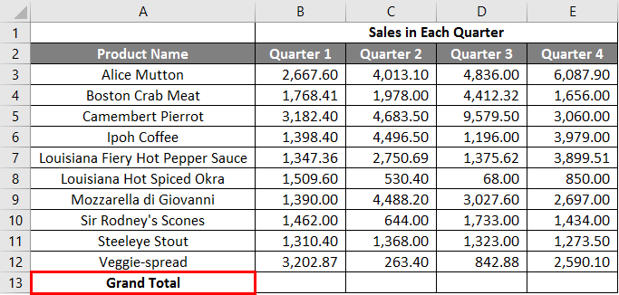
Step 8: Calculate the grand total for each quarter by summation >> apply in other cells in B13 to E13.
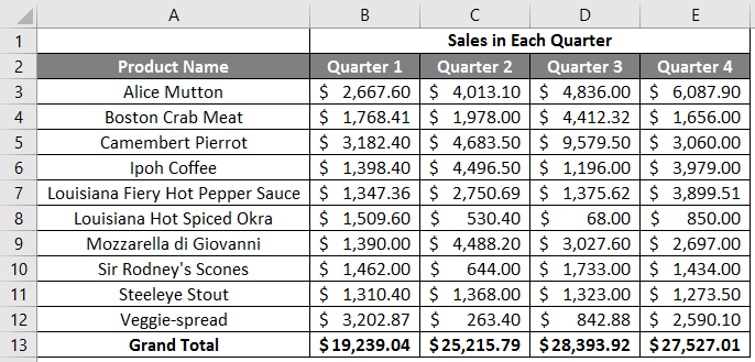
Step 9: Let’s convert the sales value into the ($) currency symbol.
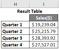
Step 10: Create a Result Table with each quarter’s total sales.
Plot the pie chart to represent the data to the client in a professional way that looks attractive. A user can change the look of the graph by just clicking on it.
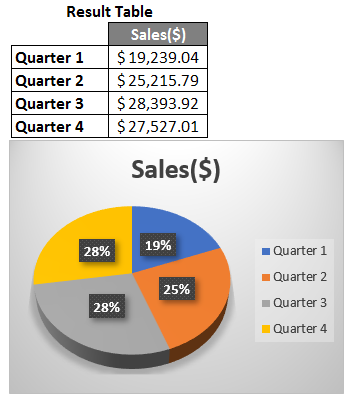
Summary of Example 2: As the user wants to create a spreadsheet to represent sales data to the client, it is done here.
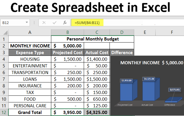
Example #3 – How to Create a Personal Monthly Budget Spreadsheet in Excel?
Let’s assume a user wants to create a spreadsheet to determine their monthly personal budget. For the year 2022, he has estimated costs and actual costs. He now wants to show his family this budget.
Let’s see how we can do this with the help of the spreadsheet.
Step 1: Open MS Excel.
Step 2: Go to Menu and select New >> Click on the Blank workbook to create a simple worksheet.
OR – Press Ctrl + N: To create a new spreadsheet.

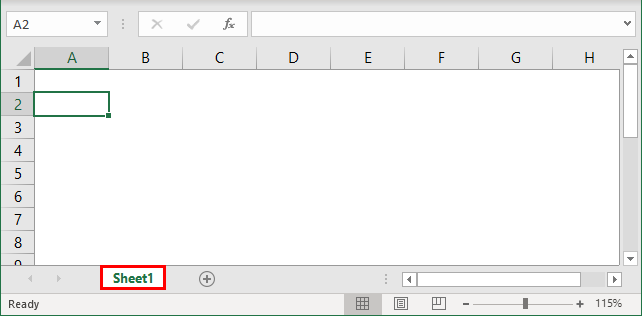
Step 3: Go to the spreadsheet work area, Sheet 2.
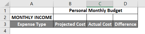
Step 4: Now create headers for Personal Monthly Budget in the first row by merging cells from B1 to D1. In row 2, give MONTHLY INCOME; in row 3, give Expense type, Projected Cost, Actual Cost, and Difference.
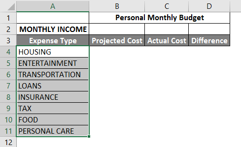
Step 5: Write down all the expenses in column A.
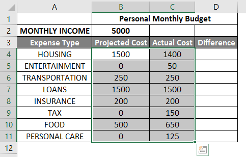
Step 6: Now, provide the monthly income, Projected cost, and Actual Cost data for each expense type.
Step 7: In the next row, put one header for Grand Total and calculate the total and difference from the project to the actual cost.
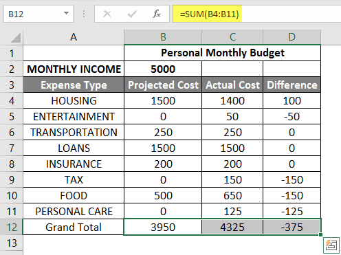
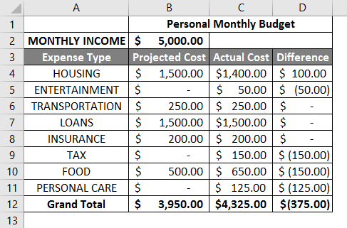
Step 8: Now highlight the header and add boundaries using toolbar graphics. >> The cost and income value in $, so make it by currency symbol.
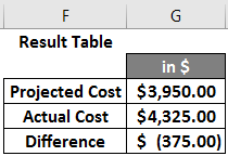
Step 9: Create a Result Table with each quarter’s total sales.
Step 10: Plot the pie chart to represent the data for the family. A user can choose one which he likes.
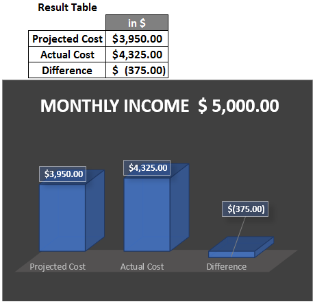
Summary of Example 3: As the user wanted to create a spreadsheet to represent monthly budget data to the family, we have created the same here. The close bracket shows in the data for the negative value.
Things to Remember
- A spreadsheet is a grid-based file designed to manage or perform any calculation on personal or business data.
- It is available in MS Office as well as Office 365.
- The workbook is the Excel lingo for ‘spreadsheet.’ MS Excel uses this term to emphasize that a single workbook can contain multiple worksheets.
How to add data in a spreadsheet Video
Recommended Articles
This article is a comprehensive guide to creating Spreadsheets in Excel. Here we have discussed how to create a Spreadsheet in Excel, examples, and a downloadable Excel template. You may also look at the following articles to learn more –
- Excel Spreadsheet Formulas
- Group Worksheets In Excel
- Excel Spreadsheet Examples
- Worksheets in Excel
На чтение 23 мин. Просмотров 18.6k.

Содержание
- Краткое руководство по текстовым функциям
- Введение
- Прочитайте это в первую очередь!
- Добавление строк
- Извлечение части строки
- Поиск в строке
- Удаление пробелов
- Длина строки
- Перевернуть текст
- Сравнение
- Сравнение строк с использованием сопоставления с шаблоном
- Заменить часть строки
- Преобразовать типы в строку (базовый)
- Преобразовать строку в число — CLng, CDbl, Val и т.д.
- Генерация строки элементов — функция строки
- Преобразовать регистр / юникод — StrConv, UCase, LCase
- Использование строк с массивами
- Форматирование строки
- Заключение
Краткое руководство по текстовым функциям
| Текстовые операции | Функции |
| Добавить две или более строки | Format or «&» |
| Построить текст из массива | Join |
| Сравнить | StrComp or «=» |
| Сравнить — шаблон | Like |
| Преобразовать в текст | CStr, Str |
| Конвертировать текст в дату | Просто: CDate Дополнительно: Format |
| Преобразовать текст в число | Просто: CLng, CInt, CDbl, Val Дополнительно: Format |
| Конвертировать в юникод, широкий, узкий | StrConv |
| Преобразовать в верхний / нижний регистр | StrConv, UCase, LCase |
| Извлечь часть текста | Left, Right, Mid |
| Форматировать текст | Format |
| Найти символы в тексте | InStr, InStrRev |
| Генерация текста | String |
| Получить длину строки | Len |
| Удалить пробелы | LTrim, RTrim, Trim |
| Заменить часть строки | Replace |
| Перевернуть строку | StrReverse |
| Разобрать строку в массив | Split |
Введение
Использование строк является очень важной частью VBA. Есть много типов манипуляций, которые вы можете делать со строками. К ним относятся такие задачи, как:
- извлечение части строки
- сравнение строк
- преобразование чисел в текст
- форматирование даты для включения дня недели
- найти символ в строке
- удаление пробелов
- парсинг в массив
- и т. д.
Хорошей новостью является то, что VBA содержит множество функций, которые помогут вам легко выполнять эти задачи.
Эта статья содержит подробное руководство по использованию строки в VBA. Он объясняет строки в простых терминах с понятными примерами кода. Изложение в статье поможет легко использовать ее в качестве краткого справочного руководства.
Если вы собираетесь использовать строки часто, я рекомендую вам прочитать первый раздел, так как он относится ко многим функциям. В противном случае вы можете прочитать по порядку или просто перейти в нужный раздел.
Прочитайте это в первую очередь!
Следующие два пункта очень важны при работе со строковыми функциями VBA.
Исходная строка не изменяется
Важно помнить, что строковые функции VBA не изменяют исходную строку. Они возвращают новую строку с изменениями, внесенными функцией. Если вы хотите изменить исходную строку, вы просто назначаете результат исходной строке. См. Раздел «Извлечение части строки» для примеров.
Как использовать Compare
Некоторые строковые функции, такие как StrComp (), Instr () и т.д. имеют необязательный параметр Compare. Он работает следующим образом:
vbTextCompare: верхний и нижний регистры считаются одинаковыми
vbBinaryCompare: верхний и нижний регистр считаются разными
Следующий код использует функцию сравнения строк StrComp () для демонстрации параметра Compare.
Sub Comp1()

    ' Печатает 0  : Строки совпадают
    Debug.Print StrComp("АБВ", "абв", vbTextCompare)
    ' Печатает -1 : Строки не совпадают
    Debug.Print StrComp("АБВ", "абв", vbBinaryCompare)

End Sub
Вы можете использовать параметр Option Compare вместо того, чтобы каждый раз использовать этот параметр. Опция сравнения устанавливается в верхней части модуля. Любая функция, которая использует параметр Compare, примет этот параметр по умолчанию. Два варианта использования Option Compare:
- Oпция Compare Text: делает vbTextCompare аргументом сравнения по умолчанию
Option Compare Text

Sub Comp2()
    ' Соответствие строк - использует vbCompareText в качестве 'аргумента сравнения
    Debug.Print StrComp("АБВ", "абв")
    Debug.Print StrComp("ГДЕ", "где")
End Sub
- Опция Compare Binary: делает vbBinaryCompare аргументом сравнения по умолчанию.
Option Compare Binary

Sub Comp2()
    ' Строки не совпадают - использует vbCompareBinary в качестве 'аргумента сравнения
    Debug.Print StrComp("АБВ", "абв")
    Debug.Print StrComp("ГДЕ", "где")
End Sub
Если Option Compare не используется, то по умолчанию используется Option Compare Binary.
Теперь, когда вы понимаете эти два важных момента о строке, мы можем продолжить и посмотреть на строковые функции индивидуально.
Добавление строк

Вы можете добавлять строки, используя оператор &. Следующий код показывает несколько примеров его использования.
Sub Dobavlenie()

    Debug.Print "АБВ" & "ГДЕ"
    Debug.Print "Иван" & " " & "Петров"
    Debug.Print "Длинный " & 22
    Debug.Print "Двойной " & 14.99
    Debug.Print "Дата " & #12/12/2015#

End Sub
В примере вы можете видеть, что различные типы, такие как даты и числа, автоматически преобразуются в строки. Вы можете увидеть оператор +, используемый для добавления строк. Разница в том, что этот оператор будет работать только со строковыми типами. Если вы попытаетесь использовать его с другим типом, вы получите ошибку.
 Это даст сообщение об ошибке: «Несоответствие типов»
    Debug.Print "Длинный " + 22
Если вы хотите сделать более сложное добавление строк, вы можете использовать функцию форматирования, описанную ниже.
Извлечение части строки
Функции, обсуждаемые в этом разделе, полезны при базовом извлечении из строки. Для чего-то более сложного можете посмотреть раздел, как легко извлечь любую строку без использования VBA InStr.
| Функция | Параметры | Описание | Пример |
| Left | строка, длина | Вернуть символы с левой стороны |
Left(«Иван Петров»,4) |
| Right | строка, длина | Вернуть символы с правой стороны |
Right(«Иван Петров»,5) |
| Mid | строка, начало, длина | Вернуть символы из середины |
Mid(«Иван Петров»,3,2) |
Функции Left, Right и Mid используются для извлечения частей строки. Это очень простые в использовании функции. Left читает символы слева, Right справа и Mid от указанной вами начальной точки.
Sub IspLeftRightMid()

    Dim sCustomer As String
    sCustomer = "Иван Васильевич Петров"

    Debug.Print Left(sCustomer, 4)  '  Печатает: Иван
    Debug.Print Right(sCustomer, 6) '  Печатает: Петров

    Debug.Print Left(sCustomer, 15)  '  Печатает: Иван Васильевич
    Debug.Print Right(sCustomer, 17)  '  Печатает: Васильевич Петров

    Debug.Print Mid(sCustomer, 1, 4) ' Печатает: Иван
    Debug.Print Mid(sCustomer, 6, 10) ' Печатает: Васильевич
    Debug.Print Mid(sCustomer, 17, 6) ' Печатает: Петров

End Sub
Как упоминалось в предыдущем разделе, строковые функции VBA не изменяют исходную строку. Вместо этого они возвращают результат в виде новой строки.
В следующем примере вы увидите, что строка Fullname не была изменена после использования функции Left.
Sub PrimerIspolzovaniyaLeft()

    Dim Fullname As String
    Fullname = "Иван Петров"

    Debug.Print "Имя: "; Left(Fullname, 4)
    ' Исходная строка не изменилась
    Debug.Print "Полное имя: "; Fullname

 End Sub
Если вы хотите изменить исходную строку, вы просто присваиваете ей возвращаемое значение функции.
Sub IzmenenieStroki()

    Dim name As String
    name = "Иван Петров"

    ' Присвойте возвращаемую строку переменной имени
    name = Left(name, 4)

    Debug.Print "Имя: "; name

 End Sub
Поиск в строке
| Функция | Параметры | Описание | Пример |
| InStr | Текст1, текст2 |
Находит положение текста |
InStr(«Иван Петров»,»в») |
| InStrRev | Проверка текста, соответствие текста |
Находит позицию текста с конца |
InStrRev(«Иван Петров»,»в») |
InStr и InStrRev — это функции VBA, используемые для поиска текста в тексте. Если текст поиска найден, возвращается позиция (с начала строки проверки) текста поиска. Когда текст поиска не найден, возвращается ноль. Если какой-либо текст имеет значение null, возвращается значение null.
InStr Описание параметров
InStr() Start[Необязат], String1, String2, Compare[Необязат]
- Start [Необязательно — по умолчанию 1]: это число, указывающее начальную позицию поиска слева
- String1: текст, в котором будем искать
- String2: текст, который будем искать
- Compare как vbCompareMethod: см. Раздел «Сравнить» для получения более подробной информации.
Использование InStr и примеры
InStr возвращает первую позицию в тексте, где найден данный текст. Ниже приведены некоторые примеры его использования.
Sub PoiskTeksta()

    Dim name As String
    name = "Иван Петров"

    ' Возвращает 3 - позицию от первой
    Debug.Print InStr(name, "а")
    ' Возвращает 10 - позиция первого "а", начиная с позиции 4
    Debug.Print InStr(4, name, "а")
    ' Возвращает 8
    Debug.Print InStr(name, "тр")
    ' Возвращает 6
    Debug.Print InStr(name, "Петров")
    ' Возвращает 0 - текст "ССС" не найдет
    Debug.Print InStr(name, "ССС")

End Sub
InStrRev Описание параметров
InStrRev() StringCheck, StringMatch, Start[Необязат], Compare[Необязат]
- StringCheck: текст, в котором будем искать
- StringMatch: Текст, который будем искать
- Start [Необязательно — по умолчанию -1]: это число, указывающее начальную позицию поиска справа
- Compare как vbCompareMethod: см. Раздел «Сравнить» для получения более подробной информации.
Использование InStrRev и примеры
Функция InStrRev такая же, как InStr, за исключением того, что она ищет с конца строки. Важно отметить, что возвращаемая позиция является позицией с самого начала. Поэтому, если существует только один экземпляр элемента поиска, InStr () и InStrRev () будут возвращать одно и то же значение.
В следующем коде показаны некоторые примеры использования InStrRev.
Sub IspInstrRev()

    Dim name As String
    name = "Иван Петров"

    ' Обе возвращают 1 - позицию, только И
    Debug.Print InStr(name, "И")
    Debug.Print InStrRev(name, "И")

    ' Возвращает 11 - вторую в
    Debug.Print InStrRev(name, "в")
    ' Возвращает 3 - первую в с позиции 9
    Debug.Print InStrRev(name, "в", 9)

    ' Returns 1
    Debug.Print InStrRev(name, "Иван")

End Sub
Функции InStr и InStrRev полезны при работе с базовым поиском текста. Однако, если вы собираетесь использовать их для извлечения текста из строки, они могут усложнить задачу. Я написал о гораздо лучшем способе сделать это в своей статье Как легко извлечь любой текст без использования VBA InStr.
Удаление пробелов
| Функция | Параметры | Описание | Пример |
| LTrim | Текст | Убирает пробелы слева |
LTrim(» Иван «) |
| RTrim | Текст | Убирает пробелы справа |
RTrim(» Иван «) |
| Trim | Текст | Убирает пробелы слева и справа |
Trim(» Иван «) |
Функции Trim — это простые функции, которые удаляют пробелы в начале или конце строки.
Функции и примеры использования триммера Trim
- LTrim удаляет пробелы слева от строки
- RTrim удаляет пробелы справа от строки
- Trim удаляет пробелы слева и справа от строки
Sub TrimStr()

    Dim name As String
    name = "  Иван Петров  "

    ' Печатает "Иван Петров  "
    Debug.Print LTrim(name)
    ' Печатает "  Иван Петров"
    Debug.Print RTrim(name)
    ' Печатает "Иван Петров"
    Debug.Print Trim(name)

End Sub
Длина строки
| Функция | Параметры | Описание | Пример |
| Len | Текст | Возвращает длину строки |
Len («Иван Петров») |
Len — простая функция при использовании со строкой. Она просто возвращает количество символов, которое содержит строка. Если используется с числовым типом, таким как long, он вернет количество байтов.
Sub IspLen()

    Dim name As String
    name = "Иван Петров"

    ' Печатает 11
    Debug.Print Len("Иван Петров")
    ' Печатает 3
    Debug.Print Len("АБВ")

    ' Печатает 4 с Long - это размер 4 байта
    Dim total As Long
    Debug.Print Len(total)

End Sub
Перевернуть текст
| Функция | Параметры | Описание | Пример |
| StrReverse | Текст | Перевернуть текст |
StrReverse («Иван Петров») |
StrReverse — еще одна простая в использовании функция. Он просто возвращает данную строку с обратными символами.
Sub RevStr()

    Dim s As String
    s = "Иван Петров"
    ' Печатает: вортеП навИ
    Debug.Print StrReverse(s)

End Sub
Сравнение
| Функция | Параметры | Описание | Пример |
| StrComp | Текст1, текст2 | Сравнивает 2 текста |
StrComp («Иван», «Иван») |
Функция StrComp используется для сравнения двух строк. Следующие подразделы описывают, как используется.
Описание параметров
StrComp() String1, String2, Compare[Необязат]
- String1: первая строка для сравнения
- String2: вторая строка для сравнения
- Compare как vbCompareMethod: см. Раздел «Сравнить» для получения более подробной информации.
StrComp Возвращаемые значения
| Возвращаемое значение | Описание |
| 0 | Совпадение строк |
| -1 | строка1 меньше строки2 |
| 1 | строка1 больше строки2 |
| Null | если какая-либо строка равна нулю |
Использование и примеры
Ниже приведены некоторые примеры использования функции StrComp.
Sub IspStrComp()

   ' Возвращает  0
   Debug.Print StrComp("АБВ", "АБВ", vbTextCompare)
   ' Возвращает 1
   Debug.Print StrComp("АБВГ", "АБВ", vbTextCompare)
   ' Возвращает -1
   Debug.Print StrComp("АБВ", "АБВГ", vbTextCompare)
   ' Returns Null
   Debug.Print StrComp(Null, "АБВГ", vbTextCompare)

End Sub
Сравнение строк с использованием операторов
Вы также можете использовать знак равенства для сравнения строк. Разница между сравнением equals и функцией StrComp:
- Знак равенства возвращает только true или false.
- Вы не можете указать параметр Compare, используя знак равенства — он использует настройку «Option Compare».
Ниже приведены некоторые примеры использования equals для сравнения строк.
Option Compare Text

Sub CompareIspEquals()

    ' Возвращает true
    Debug.Print "АБВ" = "АБВ"
    ' Возвращает true, потому что «Сравнить текст» установлен выше
    Debug.Print "АБВ" = "абв"
    ' Возвращает false
    Debug.Print "АБВГ" = "АБВ"
    ' Возвращает false
    Debug.Print "АБВ" = "АБВГ"
    ' Возвращает null
    Debug.Print Null = "АБВГ"

End Sub
Сравнение строк с использованием сопоставления с шаблоном
| Функция | Параметры | Описание | Пример |
| Like | Текст, шаблон | проверяет, имеет ли строка заданный шаблон |
«abX» Like «??X» «54abc5» Like «*abc#» |
| Знак | Значение |
| ? | Любой одиночный символ |
| # | Любая однозначная цифра (0-9) |
| * | Ноль или более символов |
| [charlist] | Любой символ в списке |
| [!charlist] | Любой символ не в списке символов |
Сопоставление с шаблоном используется для определения того, имеет ли строка конкретный образец символов. Например, вы можете проверить, что номер клиента состоит из 3 цифр, за которыми следуют 3 алфавитных символа, или в строке есть буквы XX, за которыми следует любое количество символов.
Если строка соответствует шаблону, возвращаемое значение равно true, в противном случае — false.
Сопоставление с образцом аналогично функции формата VBA в том смысле, что его можно использовать практически безгранично. В этом разделе я приведу несколько примеров, которые объяснят, как это работает. Это должно охватывать наиболее распространенные виды использования.
Давайте посмотрим на базовый пример с использованием знаков. Возьмите следующую строку шаблона.
[abc][!def]?#X*
Давайте посмотрим, как работает эта строка
[abc] — символ, который является или a, b или c
[! def] — символ, который не является d, e или f
? любой символ
# — любая цифра
X — символ X
* следуют ноль или более символов
Поэтому следующая строка действительна
apY6X
а — один из символов a,b,c
p — не один из символов d, e или f
Y — любой символ
6 — это цифра
Х — это буква Х
В следующих примерах кода показаны результаты различных строк с этим шаблоном.
Sub Shabloni()

    ' ИСТИНА
    Debug.Print 1; "apY6X" Like "[abc][!def]?#X*"
    ' ИСТИНА - любая комбинация символов после x действительна
    Debug.Print 2; "apY6Xsf34FAD" Like "[abc][!def]?#X*"
    ' ЛОЖЬ - символ не из[abc]
    Debug.Print 3; "dpY6X" Like "[abc][!def]?#X*"
    ' ЛОЖЬ - 2-й символ e находится в [def]
    Debug.Print 4; "aeY6X" Like "[abc][!def]?#X*"
    ' ЛОЖЬ - A в позиции 4 не является цифрой
    Debug.Print 5; "apYAX" Like "[abc][!def]?#X*"
    ' ЛОЖЬ - символ в позиции 5 должен быть X
    Debug.Print 1; "apY6Z" Like "[abc][!def]?#X*"

End Sub
Реальный пример сопоставления с образцом
Чтобы увидеть реальный пример использования сопоставления с образцом, ознакомьтесь с Примером 3: Проверьте, допустимо ли имя файла.
Важное примечание о сопоставлении с образцом VBA
Оператор Like использует двоичное или текстовое сравнение на основе параметра Option Compare. Пожалуйста, смотрите раздел Сравнение для более подробной информации.
Заменить часть строки
| Функция | Параметры | Описание | Пример |
| Replace | строка, найти, заменить, начать, считать, сравнивать |
Заменяет текст | Replace («Ива»,»а»,»ан») |
Replace используется для замены текста в строке другим текстом. Он заменяет все экземпляры текста, найденные по умолчанию.
Replace описание параметров
Replace() Expression, Find, Replace, Start[Необязат], Count[Необязат], Compare[Необязат]
- Expression: текст, в котором нужна замена символов
- Find: текст для замены в строке выражения
- Replace: строка для поиска замены текста поиска
- Start [Необязательно — по умолчанию 1]: начальная позиция в строке
- Count [Необязательно — по умолчанию -1]: количество замен. По умолчанию -1 означает все.
- Compare как vbCompareMethod: см. Раздел «Сравнить» для получения более подробной информации.
Использование и примеры
В следующем коде показаны некоторые примеры использования функции замены.
Sub PrimeriReplace()

    ' Заменяет все знаки вопроса (?) на точку с запятой (;)
    Debug.Print Replace("A?B?C?D?E", "?", ";")
    ' Заменить Петров на Иванов
    Debug.Print Replace("Евгений Петров,Артем Петров", "Петров", "Иванов")
    ' Заменить AX на AB
    Debug.Print Replace("ACD AXC BAX", "AX", "AB")

End Sub
На выходе:
A;B;C;D;E
Евгений Иванов,Артем Иванов
ACD ABC BAB
В следующих примерах мы используем необязательный параметр Count. Count определяет количество замен. Так, например, установка Count равной единице означает, что будет заменено только первое вхождение.
Sub ReplaceCount()

    ' Заменяет только первый знак вопроса
    Debug.Print Replace("A?B?C?D?E", "?", ";", Count:=1)
    ' Заменяет первые три знака вопроса
    Debug.Print Replace("A?B?C?D?E", "?", ";", Count:=3)

End Sub
На выходе:
A;B?C?D?E
A;B;C;D?E
Необязательный параметр Start позволяет вам вернуть часть строки. Позиция, которую вы указываете с помощью Start, — это место, откуда начинается возврат строки. Он не вернет ни одной части строки до этой позиции, независимо от того, была ли произведена замена или нет.
Sub ReplacePartial()

    ' Использовать оригинальную строку из позиции 4
    Debug.Print Replace("A?B?C?D?E", "?", ";", Start:=4)
    ' Используйте оригинальную строку из позиции 8
    Debug.Print Replace("AA?B?C?D?E", "?", ";", Start:=8)
    ' Элемент не заменен, но по-прежнему возвращаются только последние '2 символа
    Debug.Print Replace("ABCD", "X", "Y", Start:=3)

End Sub
На выходе:
;C;D;E
;E
CD
Иногда вы можете заменить только заглавные или строчные буквы. Вы можете использовать параметр Compare для этого. Он используется во многих строковых функциях. Для получения дополнительной информации об этом проверьте раздел сравнения.
Sub ReplaceCase()

    ' Заменить только заглавные А
    Debug.Print Replace("AaAa", "A", "X", Compare:=vbBinaryCompare)
    ' Заменить все А
    Debug.Print Replace("AaAa", "A", "X", Compare:=vbTextCompare)

End Sub
На выходе:
XaXa
XXXX
Многократные замены
Если вы хотите заменить несколько значений в строке, вы можете вкладывать вызовы. В следующем коде мы хотим заменить X и Y на A и B соответственно.
Sub ReplaceMulti()

    Dim newString As String

    ' Заменить А на Х
    newString = Replace("ABCD ABDN", "A", "X")
    ' Теперь замените B на Y в новой строке
    newString = Replace(newString, "B", "Y")

    Debug.Print newString

End Sub
В следующем примере мы изменим приведенный выше код для выполнения той же задачи. Мы будем использовать возвращаемое значение первой замены в качестве аргумента для второй замены.
Sub ReplaceMultiNested()

    Dim newString As String

    ' Заменить A на X, а B на Y
    newString = Replace(Replace("ABCD ABDN", "A", "X"), "B", "Y")

    Debug.Print newString

End Sub
Результатом обоих этих Subs является:
XYCD XYDN
Преобразовать типы в строку (базовый)
Этот раздел о преобразовании чисел в строку. Очень важным моментом здесь является то, что в большинстве случаев VBA автоматически конвертируется в строку для вас. Давайте посмотрим на некоторые примеры:
Sub AutoConverts()

    Dim s As String
    ' Автоматически преобразует число в строку
    s = 12.99
    Debug.Print s

    ' Автоматически преобразует несколько чисел в строку
    s = "ABC" & 6 & 12.99
    Debug.Print s

    ' Автоматически преобразует двойную переменную в строку
    Dim d As Double, l As Long
    d = 19.99
    l = 55
    s = "Значения: " & d & " " & l
    Debug.Print s

End Sub
Когда вы запустите приведенный выше код, вы увидите, что число было автоматически преобразовано в строки. Поэтому, когда вы присваиваете значение строке, VBA будет следить за преобразованием большую часть времени. В VBA есть функции преобразования, и в следующих подразделах мы рассмотрим причины их использования.
Явное преобразование
| Функция | Параметры | Описание | Пример |
| CStr | выражение | Преобразует числовую переменную в строку |
CStr («45.78») |
| Str | число | Преобразует числовую переменную в строку |
Str («45.78») |
В некоторых случаях вы можете захотеть преобразовать элемент в строку без необходимости сначала помещать его в строковую переменную. В этом случае вы можете использовать функции Str или CStr. Оба принимают выражение как функцию, и это может быть любой тип, например long, double, data или boolean.
Давайте посмотрим на простой пример. Представьте, что вы читаете список значений из разных типов ячеек в коллекцию. Вы можете использовать функции Str / CStr, чтобы гарантировать, что они все хранятся в виде строк. Следующий код показывает пример этого:
Sub IspStr()

    Dim coll As New Collection
    Dim c As Range

    ' Считать значения ячеек в коллекцию
    For Each c In Range("A1:A10")
        ' Используйте Str для преобразования значения ячейки в строку
        coll.Add Str(c)
    Next

    ' Распечатайте значения и тип коллекции
    Dim i As Variant
    For Each i In coll
        Debug.Print i, TypeName(i)
    Next

End Sub
В приведенном выше примере мы используем Str для преобразования значения ячейки в строку. Альтернативой этому может быть присвоение значения строке, а затем присвоение строки коллекции. Итак, вы видите, что использование Str здесь намного эффективнее.
Multi Region
Разница между функциями Str и CStr заключается в том, что CStr преобразует в зависимости от региона. Если ваши макросы будут использоваться в нескольких регионах, вам нужно будет использовать CStr для преобразования строк.
Хорошей практикой является использование CStr при чтении значений из ячеек. Если ваш код в конечном итоге используется в другом регионе, вам не нужно вносить какие-либо изменения, чтобы он работал правильно.
Преобразовать строку в число — CLng, CDbl, Val и т.д.
| Функция | Возвращает | Пример |
| CBool | Boolean | CBool(«True»), CBool(«0») |
| CCur | Currency | CCur(«245.567») |
| CDate | Date | CDate(«1/1/2019») |
| CDbl | Double | CDbl(«245.567») |
| CDec | Decimal | CDec(«245.567») |
| CInt | Integer | CInt(«45») |
| CLng | Long Integer | CLng(«45.78») |
| CVar | Variant | CVar(«») |
Вышеуказанные функции используются для преобразования строк в различные типы. Если вы присваиваете переменную этого типа, VBA выполнит преобразование автоматически.
Sub StrToNumeric()

    Dim l As Long, d As Double, c As Currency
    Dim s As String
    s = "45.923239"

    l = s
    d = s
    c = s

    Debug.Print "Long is "; l
    Debug.Print "Double is "; d
    Debug.Print "Currency is "; c

End Sub
Использование типов преобразования дает большую гибкость. Это означает, что вы можете определить тип во время выполнения. В следующем коде мы устанавливаем тип на основе аргумента sType, передаваемого в функцию PrintValue. Поскольку этот тип может быть прочитан из внешнего источника, такого как ячейка, мы можем установить тип во время выполнения. Если мы объявим переменную как Long, то при выполнении кода она всегда будет длинной.
Sub Test()
    ' Печатает  46
    PrintValue "45.56", "Long"
    ' Печатает 45.56
    PrintValue "45.56", ""
End Sub

Sub PrintValue(ByVal s As String, ByVal sType As String)

    Dim value

    ' Установите тип данных на основе строки типа
    If sType = "Long" Then
        value = CLng(s)
    Else
        value = CDbl(s)
    End If
    Debug.Print "Type is "; TypeName(value); value

End Sub
Если строка не является допустимым числом (т.е. Содержит символы, другие цифры), вы получаете ошибку «Несоответствие типов».
Sub InvalidNumber()

    Dim l As Long

    ' Даст ошибку несоответствия типов
    l = CLng("45A")

End Sub
Функция Val
Функция преобразует числовые части строки в правильный тип числа.
Val преобразует первые встреченные числа. Как только он встречает буквы в строке, он останавливается. Если есть только буквы, то в качестве значения возвращается ноль. Следующий код показывает некоторые примеры использования Val
Sub IspVal()

    ' Печатает 45
    Debug.Print Val("45 Новая улица")

    ' Печатает 45
    Debug.Print Val("    45 Новая улица")

    ' Печатает 0
    Debug.Print Val("Новая улица 45")

    ' Печатает 12
    Debug.Print Val("12 f 34")

End Sub
Val имеет два недостатка
- Не мультирегиональный — Val не распознает международные версии чисел, такие как запятые вместо десятичных. Поэтому вы должны использовать вышеуказанные функции преобразования, когда ваше приложение будет использоваться в нескольких регионах.
- Преобразует недопустимые строки в ноль — в некоторых случаях это может быть нормально, но в большинстве случаев лучше, если неверная строка вызывает ошибку. Затем приложение осознает наличие проблемы и может действовать соответствующим образом. Функции преобразования, такие как CLng, вызовут ошибку, если строка содержит нечисловые символы.
Генерация строки элементов — функция строки
| Функция | Параметры | Описание | Пример |
| String | число, символ | Преобразует числовую переменную в строку |
String (5,»*») |
Функция String используется для генерации строки повторяющихся символов. Первый аргумент — это количество повторений, второй аргумент — символ.
Sub IspString()

    ' Печатает: AAAAA
    Debug.Print String(5, "A")
    ' Печатает: >>>>>
    Debug.Print String(5, 62)
    ' Печатает: (((ABC)))
    Debug.Print String(3, "(") & "ABC" & String(3, ")")

End Sub
Преобразовать регистр / юникод — StrConv, UCase, LCase
| Функция | Параметры | Описание | Пример |
| StrConv | строка, преобразование, LCID |
Преобразует строку |
StrConv(«abc»,vbUpperCase) |
Если вы хотите преобразовать регистр строки в верхний или нижний регистр, вы можете использовать функции UCase и LCase для верхнего и нижнего соответственно. Вы также можете использовать функцию StrConv с аргументом vbUpperCase или vbLowerCase. В следующем коде показан пример использования этих трех функций.
Sub ConvCase()

    Dim s As String
    s = "У Мэри был маленький ягненок"

    ' верхний
    Debug.Print UCase(s)
    Debug.Print StrConv(s, vbUpperCase)

    ' нижний
    Debug.Print LCase(s)
    Debug.Print StrConv(s, vbLowerCase)

    ' Устанавливает первую букву каждого слова в верхний регистр
    Debug.Print StrConv(s, vbProperCase)

End Sub
На выходе:
У МЭРИ БЫЛ МАЛЕНЬКИЙ ЯГНЕНОК
У МЭРИ БЫЛ МАЛЕНЬКИЙ ЯГНЕНОК
у мэри был маленький ягненок
у мэри был маленький ягненок
У Мэри Был Маленький Ягненок
Другие преобразования
Как и в случае, StrConv может выполнять другие преобразования на основе параметра Conversion. В следующей таблице приведен список различных значений параметров и того, что они делают. Для получения дополнительной информации о StrConv проверьте страницу MSDN.
| Постоянные | Преобразует | Значение |
| vbUpperCase | 1 | в верхний регистр |
| vbLowerCase | 2 | в нижнем регистре |
| vbProperCase | 3 | первая буква каждого слова в верхнем регистре |
| vbWide* | 4 | от узкого к широкому |
| vbNarrow* | 8 | от широкого к узкому |
| vbKatakana** | 16 | из Хираганы в Катакану |
| vbHiragana | 32 | из Катаканы в Хирагану |
| vbUnicode | 64 | в юникод |
| vbFromUnicode | 128 | из юникода |
Использование строк с массивами
| Функция | Параметры | Описание | Пример |
| Split | выражение, разделитель, ограничить, сравнить |
Разбирает разделенную строку в массив |
arr = Split(«A;B;C»,»;») |
| Join | исходный массив, разделитель |
Преобразует одномерный массив в строку |
s = Join(Arr, «;») |
Строка в массив с использованием Split
Вы можете легко разобрать строку с разделителями в массив. Вы просто используете функцию Split с разделителем в качестве параметра. Следующий код показывает пример использования функции Split.
Sub StrToArr()

    Dim arr() As String
    ' Разобрать строку в массив
    arr = Split("Иван,Анна,Павел,София", ",")

    Dim name As Variant
    For Each name In arr
        Debug.Print name
    Next

End Sub
На выходе:
Иван
Анна
Павел
София
Если вы хотите увидеть некоторые реальные примеры использования Split, вы найдете их в статье Как легко извлечь любую строку без использования VBA InStr.
Массив в строку, используя Join
Если вы хотите построить строку из массива, вы можете легко это сделать с помощью функции Join. По сути, это обратная функция Split. Следующий код предоставляет пример использования Join
Sub ArrToStr()

    Dim Arr(0 To 3) As String
    Arr(0) = "Иван"
    Arr(1) = "Анна"
    Arr(2) = "Павел"
    Arr(3) = "София"

    ' Построить строку из массива
    Dim sNames As String
    sNames = Join(Arr, ",")

    Debug.Print sNames

End Sub
На выходе:
Иван, Анна, Павел, София
Форматирование строки
| Функция | Параметры | Описание | Пример |
| Format | выражение, формат, firstdayofweek, firstweekofyear |
Форматирует строку |
Format(0.5, «0.00%») |
Функция Format используется для форматирования строки на основе заданных инструкций. В основном используется для размещения даты или числа в определенном формате. Приведенные ниже примеры показывают наиболее распространенные способы форматирования даты.
Sub FormatDate()

    Dim s As String
    s = "31/12/2019 10:15:45"

    ' Печатает: 31 12 19
    Debug.Print Format(s, "DD MM YY")
    ' Печатает: Thu 31 Dec 2019
    Debug.Print Format(s, "DDD DD MMM YYYY")
    ' Печатает: Thursday 31 December 2019
    Debug.Print Format(s, "DDDD DD MMMM YYYY")
    ' Печатает: 10:15
    Debug.Print Format(s, "HH:MM")
    ' Печатает: 10:15:45 AM
    Debug.Print Format(s, "HH:MM:SS AM/PM")

End Sub
В следующих примерах представлены некоторые распространенные способы форматирования чисел.
Sub FormatNumbers()

    ' Печатает: 50.00%
    Debug.Print Format(0.5, "0.00%")
    ' Печатает: 023.45
    Debug.Print Format(23.45, "00#.00")
    ' Печатает: 23,000
    Debug.Print Format(23000, "##,000")
    ' Печатает: 023,000
    Debug.Print Format(23000, "0##,000")
    ' Печатает: $23.99
    Debug.Print Format(23.99, "$#0.00")

End Sub
Функция «Формат» — довольно обширная тема, и она может самостоятельно занять всю статью. Если вы хотите получить больше информации, то страница формата MSDN предоставляет много информации.
Полезный совет по использованию формата
Быстрый способ выяснить используемое форматирование — использовать форматирование ячеек на листе Excel. Например, добавьте число в ячейку. Затем щелкните правой кнопкой мыши и отформатируйте ячейку так, как вам нужно. Если вы довольны форматом, выберите «Пользовательский» в списке категорий слева. При выборе этого вы можете увидеть строку формата в текстовом поле типа. Это формат строки, который вы можете использовать в VBA.

Заключение
Практически в любом типе программирования вы потратите много времени на манипулирование строками. В этой статье рассматриваются различные способы использования строк в VBA.
Чтобы получить максимальную отдачу, используйте таблицу вверху, чтобы найти тип функции, которую вы хотите использовать. Нажав на левую колонку этой функции, вы попадете в этот раздел.
Если вы новичок в строках в VBA, то я предлагаю вам ознакомиться с разделом «Прочтите это в первую очередь» перед использованием любой из функций.
This tutorial will demonstrate how to insert a text box in Excel and Google Sheets.
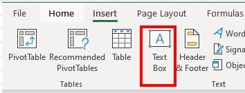
Insert a Text Box
1. In the Ribbon, select Insert > Text > Text Box.
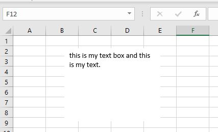
2. Click in the Excel worksheet where the text box needs to go, and drag down and to the right with the mouse to size the box accordingly.
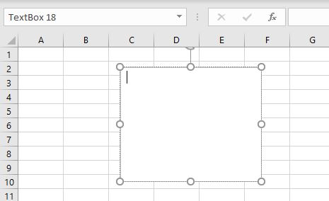
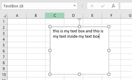
3. The cursor will now be inside the text box. To add text, just start typing!
Insert a Text Box Using the Shapes Menu
We can also insert a text box using Shapes on the Ribbon.
In the Ribbon, select Insert > Shapes > Basic Shapes > Text Box.
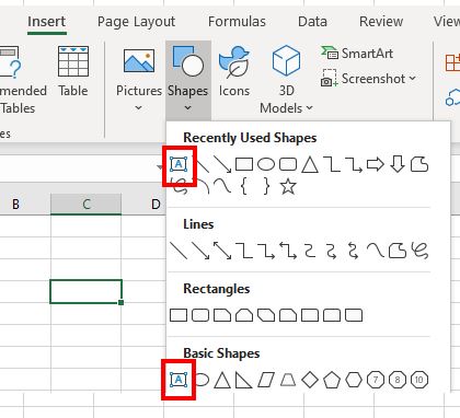
We may find that the Text Box icon is in the Recently Used Shapes group if we have recently inserted a text box into Excel.
How to Remove the Border From the Text Box
We may wish to remove the single border that is around the text box by default.
1. Click on the Text Box. A new tab will be added to the ribbon called Shape Format.
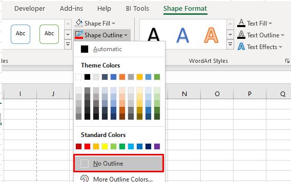
2. In the Ribbon, select Shape Format > Shape Outline > No Outline to remove the border from the text box.
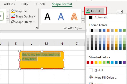
We can also use the Shape Format tab to change the border color or fill color of the text box using the Shape Fill option. We can change the color of the text inside the text box by selecting the text and then selecting Text Fill.
Insert an ActiveX Text Box
A different type of text box to insert into Excel is an ActiveX text box. This type of text box gives us greater flexibility than a text box created as a shape. One of the advantages is that we can add a scroll bar to this type of text box.
We need to have the Developer tab showing on our ribbon to insert an ActiveX text box.
1. To switch on the Developer tab, in the Ribbon, select File > Options > Customize Ribbon.
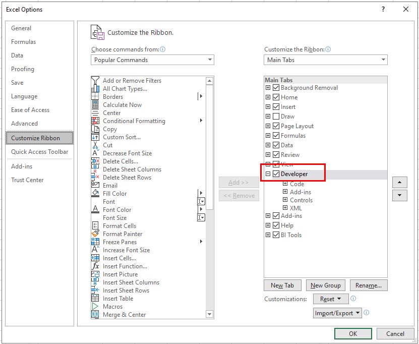
2. Check the Developer check box and click OK.
3. In the Ribbon, select Developer > Insert > ActiveX > Text Box.
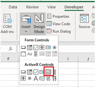
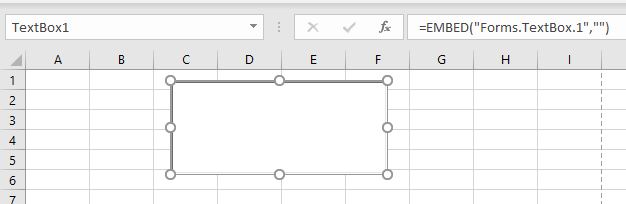
4. As we did previously, drag down and to the right with the mouse to size the box accordingly.
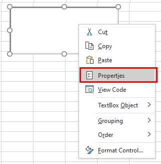
5. Right-click on the text box and then click on Properties.
OR
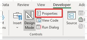
1. In the Ribbon, select Developer > Controls > Properties.
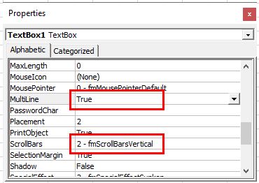
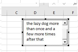
2. Select True for Multiline and then select 2 – frmScrollBarsVertical for ScrollBars.
3. Close the Properties box.
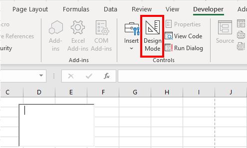
4. To enter text into the text box, click on the text box and then in the Ribbon, select Developer > Controls > Design Mode. This will switch Design Mode OFF and enable you to type text into the text box.
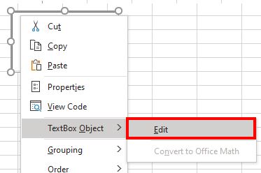
Alternatively, right-click on the text box, select TextBox Object and then click Edit.
5. Type in the desired text.
Note that it’s also possible to use VBA to insert text boxes.
How to Insert a Text Box in Google Sheets
To insert a text box into Google Sheets we need to create a drawing.
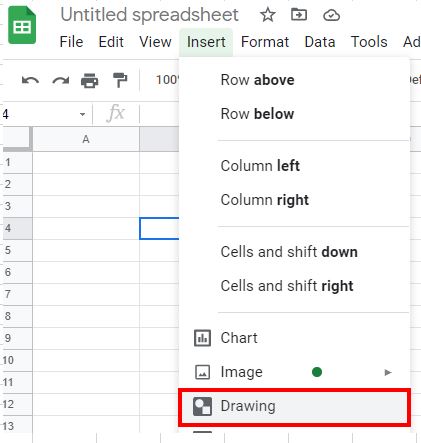
1. In the menu, select Insert > Drawing.
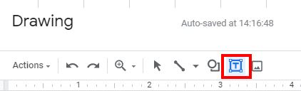
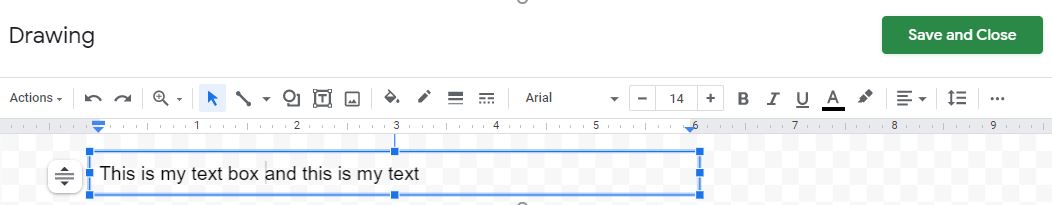
2. Select Text Box from the Drawing Toolbar.
3. Click in the drawing to create the text box.
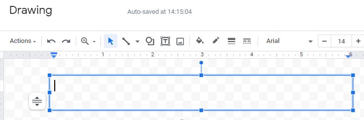
4. Type in the desired text and then click Save and Close.
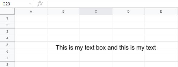
The text box will now appear in our sheet.
5. To edit the text box, click on the text box and then click on the drop down menu in the right-hand corner. Select Edit.
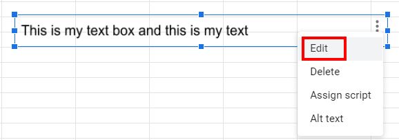
The drawing object will once again open allowing us to edit the text box.
Import or export text (.txt or .csv) files
There are two ways to import data from a text file with Excel: you can open it in Excel, or you can import it as an external data range. To export data from Excel to a text file, use the Save As command and change the file type from the drop-down menu.
There are two commonly used text file formats:
-
Delimited text files (.txt), in which the TAB character (ASCII character code 009) typically separates each field of text.
-
Comma separated values text files (.csv), in which the comma character (,) typically separates each field of text.
You can change the separator character that is used in both delimited and .csv text files. This may be necessary to make sure that the import or export operation works the way that you want it to.
Note: You can import or export up to 1,048,576 rows and 16,384 columns.
Import a text file by opening it in Excel
You can open a text file that you created in another program as an Excel workbook by using the Open command. Opening a text file in Excel does not change the format of the file — you can see this in the Excel title bar, where the name of the file retains the text file name extension (for example, .txt or .csv).
-
Go to File > Open and browse to the location that contains the text file.
-
Select Text Files in the file type dropdown list in the Open dialog box.
-
Locate and double-click the text file that you want to open.
-
If the file is a text file (.txt), Excel starts the Import Text Wizard. When you are done with the steps, click Finish to complete the import operation. See Text Import Wizard for more information about delimiters and advanced options.
-
If the file is a .csv file, Excel automatically opens the text file and displays the data in a new workbook.
Note: When Excel opens a .csv file, it uses the current default data format settings to interpret how to import each column of data. If you want more flexibility in converting columns to different data formats, you can use the Import Text Wizard. For example, the format of a data column in the .csv file may be MDY, but Excel’s default data format is YMD, or you want to convert a column of numbers that contains leading zeros to text so you can preserve the leading zeros. To force Excel to run the Import Text Wizard, you can change the file name extension from .csv to .txt before you open it, or you can import a text file by connecting to it (for more information, see the following section).
-
Import a text file by connecting to it (Power Query)
You can import data from a text file into an existing worksheet.
-
On the Data tab, in the Get & Transform Data group, click From Text/CSV.
-
In the Import Data dialog box, locate and double-click the text file that you want to import, and click Import.
-
In the preview dialog box, you have several options:
-
Select Load if you want to load the data directly to a new worksheet.
-
Alternatively, select Load to if you want to load the data to a table, PivotTable/PivotChart, an existing/new Excel worksheet, or simply create a connection. You also have the choice of adding your data to the Data Model.
-
Select Transform Data if you want to load the data to Power Query, and edit it before bringing it to Excel.
-
If Excel doesn’t convert a particular column of data to the format that you want, then you can convert the data after you import it. For more information, see Convert numbers stored as text to numbers and Convert dates stored as text to dates.
Export data to a text file by saving it
You can convert an Excel worksheet to a text file by using the Save As command.
-
Go to File > Save As.
-
Click Browse.
-
In the Save As dialog box, under Save as type box, choose the text file format for the worksheet; for example, click Text (Tab delimited) or CSV (Comma delimited).
Note: The different formats support different feature sets. For more information about the feature sets that are supported by the different text file formats, see File formats that are supported in Excel.
-
Browse to the location where you want to save the new text file, and then click Save.
-
A dialog box appears, reminding you that only the current worksheet will be saved to the new file. If you are certain that the current worksheet is the one that you want to save as a text file, click OK. You can save other worksheets as separate text files by repeating this procedure for each worksheet.
You may also see an alert below the ribbon that some features might be lost if you save the workbook in a CSV format.
For more information about saving files in other formats, see Save a workbook in another file format.
Import a text file by connecting to it
You can import data from a text file into an existing worksheet.
-
Click the cell where you want to put the data from the text file.
-
On the Data tab, in the Get External Data group, click From Text.
-
In the Import Data dialog box, locate and double-click the text file that you want to import, and click Import.
Follow the instructions in the Text Import Wizard. Click Help
 on any page of the Text Import Wizard for more information about using the wizard. When you are done with the steps in the wizard, click Finish to complete the import operation.
 -
In the Import Data dialog box, do the following:
-
Under Where do you want to put the data?, do one of the following:
-
To return the data to the location that you selected, click Existing worksheet.
-
To return the data to the upper-left corner of a new worksheet, click New worksheet.
-
-
Optionally, click Properties to set refresh, formatting, and layout options for the imported data.
-
Click OK.
Excel puts the external data range in the location that you specify.
-
 on any page of the Text Import Wizard for more information about using the wizard. When you are done with the steps in the wizard, click Finish to complete the import operation.
If Excel does not convert a column of data to the format that you want, you can convert the data after you import it. For more information, see Convert numbers stored as text to numbers and Convert dates stored as text to dates.
Export data to a text file by saving it
You can convert an Excel worksheet to a text file by using the Save As command.
-
Go to File > Save As.
-
The Save As dialog box appears.
-
In the Save as type box, choose the text file format for the worksheet.
-
For example, click Text (Tab delimited) or CSV (Comma delimited).
-
Note: The different formats support different feature sets. For more information about the feature sets that are supported by the different text file formats, see File formats that are supported in Excel.
-
-
Browse to the location where you want to save the new text file, and then click Save.
-
A dialog box appears, reminding you that only the current worksheet will be saved to the new file. If you are certain that the current worksheet is the one that you want to save as a text file, click OK. You can save other worksheets as separate text files by repeating this procedure for each worksheet.
-
A second dialog box appears, reminding you that your worksheet may contain features that are not supported by text file formats. If you are interested only in saving the worksheet data into the new text file, click Yes. If you are unsure and would like to know more about which Excel features are not supported by text file formats, click Help for more information.
For more information about saving files in other formats, see Save a workbook in another file format.
The way you change the delimiter when importing is different depending on how you import the text.
-
If you use Get & Transform Data > From Text/CSV, after you choose the text file and click Import, choose a character to use from the list under Delimiter. You can see the effect of your new choice immediately in the data preview, so you can be sure you make the choice you want before you proceed.
-
If you use the Text Import Wizard to import a text file, you can change the delimiter that is used for the import operation in Step 2 of the Text Import Wizard. In this step, you can also change the way that consecutive delimiters, such as consecutive quotation marks, are handled.
See Text Import Wizard for more information about delimiters and advanced options.
If you want to use a semi-colon as the default list separator when you Save As .csv, but need to limit the change to Excel, consider changing the default decimal separator to a comma — this forces Excel to use a semi-colon for the list separator. Obviously, this will also change the way decimal numbers are displayed, so also consider changing the Thousands separator to limit any confusion.
-
Clear Excel Options > Advanced > Editing options > Use system separators.
-
Set Decimal separator to , (a comma).
-
Set Thousands separator to . (a period).
When you save a workbook as a .csv file, the default list separator (delimiter) is a comma. You can change this to another separator character using Windows Region settings.
Caution: Changing the Windows setting will cause a global change on your computer, affecting all applications. To only change the delimiter for Excel, see Change the default list separator for saving files as text (.csv) in Excel.
-
In Microsoft Windows 10, right-click the Start button, and then click Settings.
-
Click Time & Language, and then click Region in the left panel.
-
In the main panel, under Regional settings, click Additional date, time, and regional settings.
-
Under Region, click Change date, time, or number formats.
-
In the Region dialog, on the Format tab, click Additional settings.
-
In the Customize Format dialog, on the Numbers tab, type a character to use as the new separator in the List separator box.
-
Click OK twice.
-
In Microsoft Windows, click the Start button, and then click Control Panel.
-
Under Clock, Language, and Region, click Change date, time, or number formats.
-
In the Region dialog, on the Format tab, click Additional settings.
-
In the Customize Format dialog, on the Numbers tab, type a character to use as the new separator in the List separator box.
-
Click OK twice.
Note: After you change the list separator character for your computer, all programs use the new character as a list separator. You can change the character back to the default character by following the same procedure.
Need more help?
You can always ask an expert in the Excel Tech Community or get support in the Answers community.
See Also
Import data from external data sources (Power Query)
Need more help?
Want more options?
Explore subscription benefits, browse training courses, learn how to secure your device, and more.
Communities help you ask and answer questions, give feedback, and hear from experts with rich knowledge.
Sometimes you may have the text and numeric data in the same cell, and you may have a need to separate the text portion and the number portion in different cells.
While there is no inbuilt method to do this specifically, there are some Excel features and formulas you can use to get this done.
In this tutorial, I will show you 4 simple and easy ways to separate text and numbers in Excel.
Let’s get to it!
Separate Text and Numbers Using Flash Fill
Below I have the employee data in column A, where the first few alphabets indicate the department of the employee and the numbers after it indicates the employee number.

From this data, I want to separate the text part and the number part and get these into two separate columns (columns B and C).
The first method that I want to show you to separate text and numbers in Excel is by using Flash Fill.
Flash Fill (introduced in Excel 2013) works by identifying patterns based on user input.
So if I manually enter the expected result in column B, Flash Fill will try and decipher the pattern and give me the result for all the cells in that column.
Below are the steps to separate the text part from the cell and get it in column B:
- Select cell B2
- Manually enter the expected result in cell B2, which would be MKT

- With cell B2 selected, place the cursor at the bottom right part of the selection. You’ll notice that the cursor changes into a plus icon (this is called Fill Handle)

- Hold the left mouse/trackpad key and drag the Fill Handle to fill the cells. Don’t worry if the cells are filled with the same text
- Click on the Auto Fill Options icon and then select the ‘Flash Fill’ option

The above steps would extract the text part from the cells in column A and give you the result in column B.

Note that in some cases, Flash Fill may not be able to identify the right pattern. In such cases, it would be best to enter the expected result in two or three cells, use the Fill Handle to fill the entire column, and then use Flash Fill on this data.
You can follow the same process to extract the numbers in column C. All you need to do is enter the expected result in cell C2 (step 2 in the process laid out above)
Note that the result you get from Flash Fill is static and would not update in case you change the original data in column A. If you want the result to be dynamic, you can use the formula method covered next.
Separate Text and Numbers Using Formula
Below I have the employee data in column A and I want to use a formula to extract only the text part and put it in column B and extract the number part and put it in column C.
Since the data is not consistent (i.e., the alphabets in the department code and the numbers in the employee number are not of the consistent length), I cannot use the LEFT or RIGHT function to extract only the text portion or only the number portion.
Below is the formula that will extract only the text portion from the left:
=LEFT(A2,MIN(IFERROR(FIND({0,1,2,3,4,5,6,7,8,9},A2),""))-1)

And below is the formula that will extract all the numbers from the right:
=MID(A2,MIN(IFERROR(FIND({0,1,2,3,4,5,6,7,8,9},A2),"")),100)

How does this formula work?
Let me first explain the formula that we use to separate the text part on the left.
=LEFT(A2,MIN(IFERROR(FIND({0,1,2,3,4,5,6,7,8,9},A2),””))-1)
The FIND part in the formula finds the position of digits 0 to 9 in cell A2. In case it finds that digit in cell A2, it returns the position of that digit, and in case it is not able to find that digit, then it returns the value error (#VALUE!)
For cell A2, it gives a result as shown below:
{#VALUE!,4,#VALUE!,#VALUE!,#VALUE!,6,#VALUE!,5,#VALUE!,#VALUE!}
- For 0, it returns #VALUE! as it cannot find this digit in cell A2
- For 1, it returns 4 as that is the position of the first occurrence of 1 in cell A2
- and so on…
This FIND formula is then wrapped inside the IFERROR function, which removes all the value errors but leaves the numbers.
The result of it looks like as shown below:
{“”,4,””,””,””,6,””,5,””,””}
The MIN function then goes through the above result and gives us the minimum value from the results. Since each number in the array represents the position of that corresponding number, the minimum value tells us where the numerical value starts in the cell.
Now that we know where the numerical values start, I have used the LEFT function to extract everything before this position (which would be all the text in the cell).
Similarly, you can use the same formula with a minor tweak to extract all the numbers after the text. To extract the numbers, where we know the starting position of the first digit, use the MID function to extract everything starting from that position.
And what if the situation is reversed – where we have the numbers first and the text later and we want to separate the numbers and text?
You can still use the same logic with one minor change – instead of finding the minimum value that gives us the position of the 1st digit in the cell, you need to use the MAX function To find the position of the last digit in this cell. Once you have it, you can again use the LEFT function or the MID function to separate the numbers and text.
Separate Text and Numbers Using VBA (Custom Function)
While you can use the formulas shown above to separate the text and numbers in a cell and extract these into different cells – if this is something you need to do quite often, you also have the option to create your own custom function using VBA.
The benefit of creating your own function would be that it would be a lot easier to use (with just one function that takes only one argument).
You can also save this custom function VBA code into the Personal Macro Workbook so that it would be available in all your Excel workbooks.
Below the VBA code that could create a function ‘GetNumber’ that would take the cell reference as the input argument, extract all the numbers in the cell, and give it as the result.
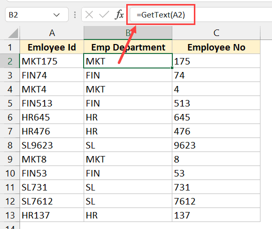
'Code created by Sumit Bansal from https://trumpexcel.com
'This code will create a function that can separate numbers from a cell
Function GetNumber(CellRef As String)
Dim StringLength As Integer
StringLength = Len(CellRef)
For i = 1 To StringLength
If IsNumeric(Mid(CellRef, i, 1)) Then Result = Result & Mid(CellRef, i, 1)
Next i
GetNumber = Result
End Function
And below the VBA code that would create another function ‘GetText’ that would take the cell reference as the input argument and give you all the text from that cell
'Code created by Sumit Bansal from https://trumpexcel.com
''This code will create a function that can separate text from a cell
Function GetText(CellRef As String)
Dim StringLength As Integer
StringLength = Len(CellRef)
For i = 1 To StringLength
If Not (IsNumeric(Mid(CellRef, i, 1))) Then Result = Result & Mid(CellRef, i, 1)
Next i
GetText = Result
End Function
Below are the steps to add this code to your excel workbook so that this function becomes available for you to use in the worksheet:
- Click the Developer tab in the ribbon
- Click on the Visual Basic icon

- In the Visual Basic editor that opens up, you would see the Project Explorer on the left. This would have the workbook and the worksheet names of your current Excel workbook. If you don’t see this, click on the View option in the menu and then click on Project Explorer

- Select any of the sheet names (or any object) for the workbook in which you want to add this function
- Click on the Insert option in the top toolbar and then click on Module. This will insert a new module for that workbook

- Double click on the module icon in ‘Project Explorer’. This will open the module code window.

- Copy and paste the above custom function code into the module code window

- Close the VB Editor
With the above steps, we have added the custom function code to the Excel workbook.
Now you can use the functions =GETNUMBER or =GETTEXT just like any other worksheet function.
Note – Once you have the macro code in the module code window, you need to save the file as a Macro Enabled file (with the .xlsm extension instead of the .xlsx extension)
If you often have a need to separate text numbers from cells in Excel, it would be more efficient if you copy these VBA codes for creating these custom functions, and save these in your Personal Macro Workbook.
You can learn how to create and use Personal Macro Workbook in this tutorial I created earlier.
Once you have these functions in the Personal Macro Workbook, you would be able to use these on any Excel workbook on your system.
One important thing to remember when using functions that are stored in Personal Macro Workbook – you need to prefix the function name with =PERSONAL.XLSB!. For example, if I want to use the function GETNUMBER in a workbook in Excel, and I have saved the code for it in the postal macro workbook, I will have to use =PERSONAL.XLSB!GETNUMBER(A2)
Separate Text and Numbers Using Power Query
Power Query is slowly becoming my favorite feature in Excel.
If you’re already using Power Query as a part of your workflow, and you have a data set where you want to separate the text and numbers into separate columns, Power Query will do it in a few clicks.
When you have your data in Excel and you want to use Power Query to transform that data, one prerequisite is to convert that data into an Excel Table (or a named range).
Below I have an Excel Table that contains the data where I want to separate the text and number portions into separate columns.

Here are the steps to do this:
- Select any cell in the Excel Table
- Click the Data tab in the ribbon

- In the Get and Transform group, click on the ‘From Table/Range’

- In the Power Query editor that opens up, select the column from which you want to separate the numbers and text
- Click the Transform tab in the Power Query ribbon

- Click on the Split Column option

- Click on ‘By Non Digit to Digit’ option.

- You’ll see that the column has been split into two columns where one has only the text and the other only has the numbers

- [Optional] Change the column names if you want
- Click the Home tab and then click on Close and Load. This will insert a new sheet and give us the output as an Excel Table.

The above steps would take the data from the Excel Table we originally had, use Power Query to split the column and separate the text and the number parts into two separate columns, and then give us back the output in a new sheet in the same workbook.

Note that we used the option ‘By Non-Digit to Digit’ option in step 7, which means that every time there is a change from a non-digit character to a digit, a split would be made. If you have a dataset where the numbers are first followed by text, you can use the ‘By Digit to Non-Digit’ option
Now let me tell you the best part about this method. Your original Excel Table (which is the data source) is connected to the output Excel Table.
So if you make any changes in your original data, you don’t need to repeat the entire process. You can simply go to any cell in the output Excel Table, right click and then click on Refresh.
Power query would run in the back end, check the entire original data source, do all the transformations that we did in the steps above, and update your output result data.
This is where Power Query really shines. If there is a set of transformations that you often need to do on a data set, you can use Power Query to do that transformation once and set the process. Excel would create a connection between the original data source and the resulting output data and remember all the steps you had taken to transform this data.
Now, if you get a new data set you can simply put it in the place of your original data and refresh the query, and you will get the result in a few seconds. Alternatively, you can simply change the source in Power Query from the existing Excel table to some other Excel Table (in same or different workbook).
So these are four simple ways you can use to separate numbers and text in Excel. if this is a once-in-a-while activity, you’re better off using Flash Fill or the formula method.
And in case this is something you need to do quite often, then I would suggest you consider the VBA method where we created a custom function or the Power Query method.
I hope you found this Excel tutorial useful.
Other Excel tutorials you may also like:
- Separate First and Last Name in Excel (Split Names Using Formulas)
- How to Convert Numbers to Text in Excel
- Convert Text to Numbers in Excel – A Step By Step Tutorial
- How to Compare Text in Excel
- How to Quickly Combine Cells in Excel
- How to Combine First and Last Name in Excel
- How to Extract the First Word from a Text String in Excel (3 Easy Ways)
- Extract Numbers from a String in Excel (Using Formulas or VBA)
- How to Extract a Substring in Excel (Using TEXT Formulas)
How to Create a Spreadsheet in Excel
The world’s most robust pure spreadsheet application, Excel, comes as part of both Microsoft Office and Office 365. There are two main differences between the two offerings: First, Microsoft Office is an on-premise application whereas Office 365 is a cloud-based app suite. Second, Office is a one-time payment, and Office 365 is a monthly subscription. Excel is available for both Mac and PC.
«Spreadsheets keep you organized. Rows and columns, formatting, formulas, filtering. That’s the building blocks of structure and overview.» — Kasper Langmann, Co-founder of Spreadsheeto
Unique Features of Excel
With over 400 functions, Excel is more or less the most comprehensive spreadsheet option when it comes to pure calculations. It also has strong visualization abilities, including conditional formatting, Pivot Tables, SmartArt, graphs, and charts. Home and business users alike can create powerful spreadsheets and reports to track data and inform their decisions.
One powerful Excel feature is Macro, little scripts and recordings you can create to make the program perform different actions automatically. While no other spreadsheet program has this type of feature, it is complex and can pose difficulty for beginners.
Excel also has close tie-ins with Microsoft Access, a database program, which can add power. In general, Excel integrates best with databases and any dataset requiring many calculations per workbook.
Understanding Your Main Screen
When you first open Excel in Office 365 or a newer version of Microsoft Office, you’ll see a basic screen. Here are the key features in this view:
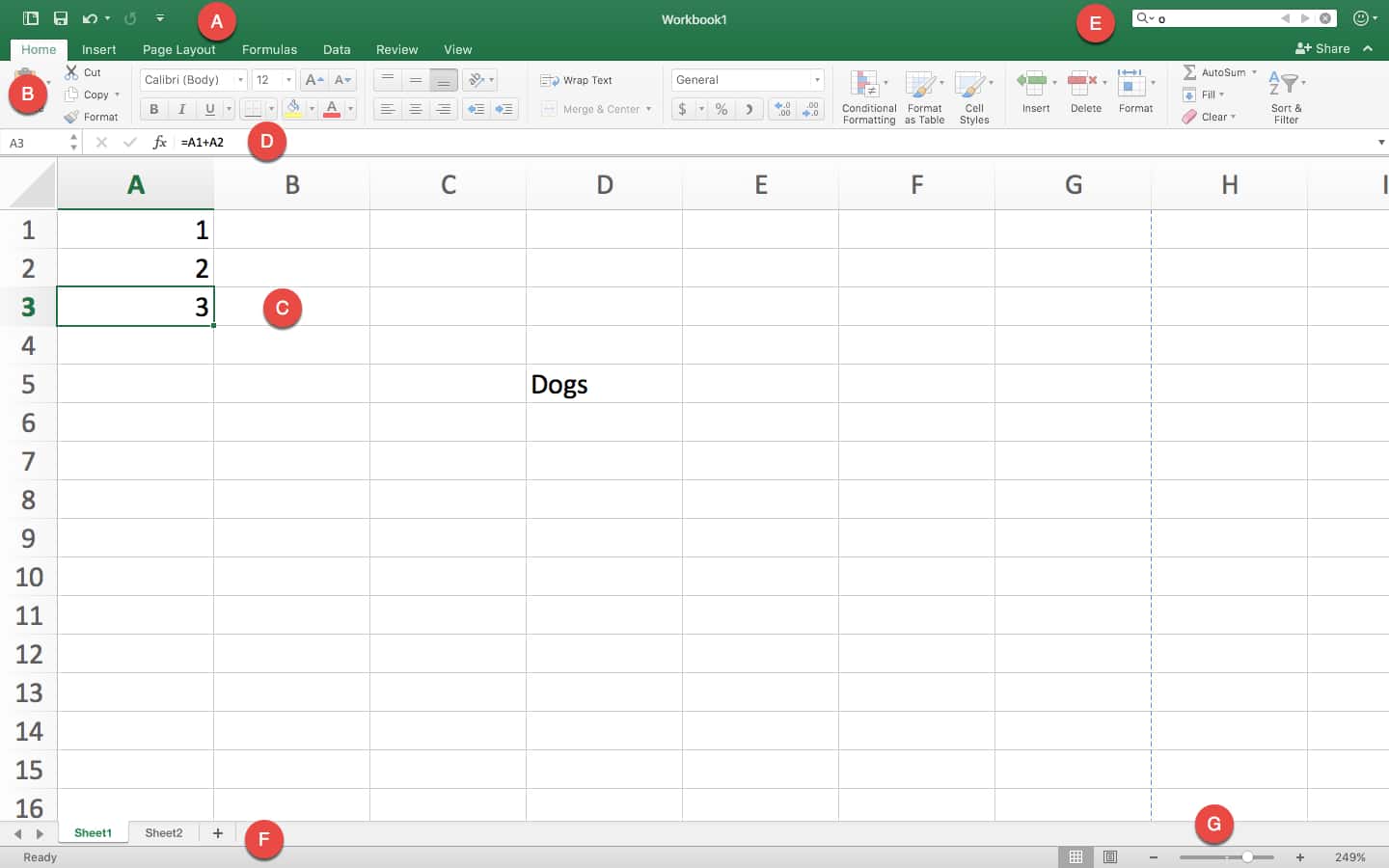
A. Basic App Functions: From left to right along this top green banner you’ll find icons to: reopen the Create a Workbook page; save your work; undo the last action performed and display which actions were recorded; redo a step that’s been undone; select which tools appear below.
B. Ribbon:This grey area is called the Ribbon, and contains tools for entering, manipulating, and visualizing data. There are also tabs that focus on specific features. Home is selected by default; click on the Insert, Page Layout, Formulas, Data, Review, or View tab to reveal a set of tools unique to each tab. We’ll cover this more in the “Navigating the Ribbon” section later on.
C. Spreadsheet Work Area: By default the work area is a grid. Along the top are column headers A through Z (and beyond), and along the left side are numbered row headers. Each rectangle in the spreadsheet is called a cell, and they are each named according to their column letter and row number. For example, the cell selected here is A3.
D. Formula Bar: The Formula Bar displays the information contained within a highlighted single cell or range of cells. If in cell A1 you entered “1” as a value, “1” will appear in the Formula Bar. Plain text that you enter in a cell will also appear in the Formula Bar.
There are cases where what you see in the Formula Bar is different than what’s in the cell. For example, let’s say A1 = 1 and A2 = 2. If you create a formula in A3 that equals A1 + A2, then the A3 cell in your worksheet would show “3,” but the Formula Bar would show “=A1+A2.” This is important when you’re trying to move cells to other parts of your worksheet — remember that the display “value” of a cell isn’t necessarily what the cell contains.
That said, other formulas that reference a cell will take into account the current value of a cell. If A4 = A3 + 1, then it would be equal to 4, because it stacks the formula of A3 (A1 + A2) with A4 = A3 + 1. Formulas can reference other formulas multiple times.
E. Search Bar: Simply type the value you want to find to highlight all cells containing that value. It doesn’t have to be an exact match. For instance, if you searched for “o,” a cell labeled “Dogs” would appear among your search results.
F. Sheet Tabs: This is where the different sheets in your workbook can be found. Each sheet gets its own tab, which you can name yourself. These can be useful to separate out data so that one sheet doesn’t get too overwhelming. For example, you might have an annual budget, where each month is a column, and each row is a type of expense. Instead of keeping every single year you track on one sheet and scrolling horizontally, you can make each tab a different year containing 12 months only.
Note that data from different sheets in the same workbook can be referenced for formulas. For example, if you have two sheets, Sheet1 and Sheet2, you could bring Sheet2 data into Sheet1. If you wanted cell A1 in Sheet1 to equal the A1 in Sheet2, you’d enter this formula into A1: “=Sheet2!A1”. The exclamation mark calls on the previous sheet referenced before locating the data.
G. Viewability Options: The left icon is Normal which shows the worksheet as it appears in the image above, and the right icon is Page Layout, which divides your worksheet into pages resembling how it would look when printed, with the option to add headers. The slider with the “-” and “+” on it is for scale or zoom-level. Drag the slider left or right to zoom in or out.
Navigating the Ribbon
The Home tab is where you manage the formatting and appearance of your sheet, along with some simple formulas you’ll always need.
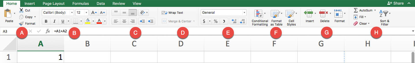
A. Copy and Paste Tools: Use these tools to quickly duplicate data and format styles in the spreadsheet. The Copy tool can either copy a selected cell or group of cells, or copy an area of the spreadsheet that you’ll use as a picture in another document. The Cut tool moves the selection of cells to a new destination rather than duplicating it.
The Paste tool can paste anything in your clipboard into the selected cell, and typically retains everything including the value, formula, and format. However, Excel has a wealth of pasting options: you can access these by clicking the down arrow next to the Paste icon. You can paste what you’ve copied as a picture. You can also paste what you’ve copied as values only, so that instead of duplicating the formula of a copied cell, you duplicate the final value shown in the cell.
The Format paintbrush copies everything related to the formatting of a selected cell. When you select a cell and click Format, you can then highlight a whole range of cells, and each one will take on the formatting of the original cell, without changing their values.
B. Visual Formatting Tools: Many of these tools are similar to those found in Microsoft Word. You can use the formatting tools to change the font, size, and color of typed words, and make them bold, italicized, or underlined. It also has a couple spreadsheet-specific formatting options. You can choose which sides of the cell get additional borders, and their style and thickness. You can also change the highlight color of the entire cell. This is useful for creating visually-appealing borders or differentiating rows or columns on large sheets, or for highlighting a particular cell that you want to accentuate.
C. Position Formatting Tools: Align cell data to the top, bottom, or middle of the cell. There is also an option for angling the values displayed, which can make it easier to read. The bottom row has familiar options for left, center, and right alignment. There are also indent right and left buttons.
D. Multi-cell Formatting Features: This section contains two very important features that solve common problems for new Excel users. The first is Wrap Text. Normally, when you enter text into a cell that extends beyond the size of the cell, it spills into the next cell. For example, if you type “Budgeted Items” into A1, some of the word “Items” spills into B1. Then, if you type into B1, you cover up any characters from A1 that extended into B1. The extra text from cell A1 still exists, but now it is hidden. If you don’t want to widen the cells, click the Wrap Text icon on A1 — this will split “Budgeted Items” into two stacked lines instead of one within A1. This makes the entire row taller to accommodate the content. Now, typing into B1 won’t cover up existing text.
The other tool in this section is Merge and Center. There are instances when you may want to combine several cells and have them act as one long cell. For example, you might want a header for an entire table to be clear and easy to read. Select all the cells you want combined, click Merge, and then type your header and format it. Though the default setting for headers is centered text, simply click the drop-down arrow to select different merging and unmerging options.
E. Numbers-based Format Settings: A drop-down menu has options for number formatting. For example, currency places everything you select into “$0.00” format, and percent turns .5 or ½ into “50%”, date options. These are the basic format options, but you can select More Number Formats from the drop-down menu to get more specialty use cases (different countries’ currencies, or adding the “(xxx)xxx-xxxx” formatting to phone number sequences). Often, you may use these tools on entire columns to make all data in one category behave the same way.
F. Table or Sheet Formatting: Format as Table and Cell Styles allow you to use presets or customize tables (for example, with alternating row colors and highlighted header bars). Select your data range and choose a style to standardize formatting.
Conditional formatting is a bit more complex. Use the drop-down menu to select from a range of options, like inserting helpful visual icons to represent status or completion, or changing the color of different rows. Most important are the conditional rules, which are created with a simple logic. For example, let’s say you have a column with data in A1 through A3, and A4 holds the sum of these three cells. You could place formatting on A4 with a rule that says “if A4 > 0, then highlight A4 green.” Then, you could add another rule that says “if A4 < 0, then highlight A4 red.” Now you have a quick visual reference where green = a positive number and red = a negative number, which will change based on what you enter into A1, A2, and A3.
G. Row and Column Formatting Tools: The Insert drop-down menu puts cells, rows, or columns before or after a selected area on the sheet, and Delete removes them. The Format drop-down lets you change the height of rows and the width of columns. It also has options for hiding and unhiding certain sections.
H. Miscellaneous Tools: Starting at the top left, there’s AutoSum, which allows you to select a swath of cells and place the sum in the cell located right below or directly to the right of the last selected data point. You can use the drop-down to change the function to calculate the average, display the maximum, minimum, or the count of numbers selected.
Use Fill to take a cell’s contents and extend them in any direction for as many cells as you want. If the cell contains a value, Fill will simply copy the value over and over again. If it contains a formula, it will recalculate its relative position for each new cell. If the first cell equals A1+B1, then the next would equal A2+B2, and so on.
The Clear button lets you either clear the value, or just clear cell formatting.
Sort & Filter tools let you choose what to display, and in what order. At the base level, this tool sorts cells containing text from A to Z, and cells containing numbers from lowest to highest. It can also sort by color or icon. Sorting and filtering helps surface only the data you need.
Use the Insert tab to add extra elements to your Excel workbook that go beyond text and colors.
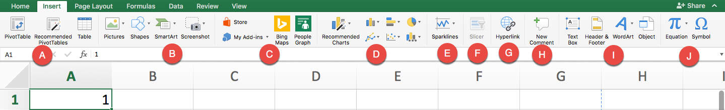
A. These tools control PivotTables, an important Excel function. Think of PivotTables as “reports,” a quick way to view all your data, analyze trends, and draw conclusions. By selecting at least two rows of data and clicking on PivotTable, you can quickly generate a visually-appealing table. Going through this process launches the PivotTable Builder, which helps you select columns to include, sort them, and drag-and-drop them to quickly construct your table. They can include collapsible rows to make reports interactive and uncluttered. There is also a button for Recommended PivotTables, which can help when you don’t know where to start.
Table builds a simple table that includes any number of columns you select. Rather than placing the table elsewhere on the worksheet, it turns the data into a table on the spot, and applies customizable color formatting.
B. This section lets you insert visual elements, like picture files, pre-built shapes, and SmartArt. You can add shapes and resize, recolor, and reposition them to create intuitive data sets and reports. SmartArt objects are prebuilt diagrams that you can insert text and information into. They’re great for representing what the data says in another place on your workbook.
C. These tools are for inserting elements from other Microsoft products, like Bing Maps, pre-built information cards about People (from Microsoft accounts only), and add-ins from their store.
D. Use these tools to create charts and graphs. Most of them work only if you select one or more data sets (numbers only, with words for headers or categories). Charts and graphs function like you’d expect — just select the data you want to visualize, then select your desired type of visual (bar charts, scatter plots, pie charts, or line graphs). Creating one will bring up formatting options where you can change the color, labels, and more.
E. Sparklines are more simplistic graphs that can fit in as little as one cell. You can place them next to data for a small, quick visual representation.
F. Slicers are big lists of buttons that make your data more interactive. You can select a PivotTable you’ve created, and then create a slicer from it — this allows a viewer to click on buttons that correlate to the data they want to filter.
G. This hyperlink tool allows you to make a cell or table into a clickable link. Once a viewer clicks on the affected cell(s), they’ll be taken to whatever website or intranet site you select.
H. Recent versions of Excel allow for better collaboration — insert comments on any cell or range of cells to add more context. You can open or close the comments so the worksheet doesn’t get too cluttered.
I. A Text Box is useful when you’re creating a report and don’t want typed words to behave like cells. It makes it easy to move your text around, rather than cutting and pasting cells (which could potentially mess up the formatting of real data). The next area is for Headers & Footers, which will take you to the page layout view — here you can add headers and footers for the entire page. WordArt, on the other hand, lets you embellish text. Insert Object lets you place entire files (Word documents, PDFs, etc.) into the worksheet.
J. This section lets you insert Equations and Symbols. Use equations to write a math equation with fractions, variables, and more that you can place in your sheet like a Text Box. For instance, this can be helpful for explaining how a portion of a table was calculated in a report. Symbols, on the other hand, can be inserted directly into cells, and include all non-standard characters from most languages, as well as emojis.
The Page Layout tab has everything you need to change the structural parts of your worksheet, especially for purposes of printing or presenting.
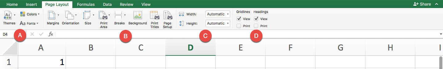
A. Use these buttons to quickly adjust the visual style of your entire sheet. You can regulate the fonts and colors, and use the Themes section to quickly apply it to every table, PivotTable, and SmartArt element for a clean, well-designed sheet.
B. These are print options. You can change the margin for printing, whether you want a vertical or horizontal print alignment, which cells in your sheet you want to print, where you’d like page breaks, and whether it has a background (to place your company name, for example). You can also start giving each page a heading using the Print Titles button, and the order to print each section.
C. This lets you choose how many pages across and how many pages down you’d like to print.
D. This section lets you toggle whether the automatic grids appear for working on the sheet and for printing it, along with the row and column headings (A, B, C, 1, 2, 3, etc).
The Formulas tab stores nearly everything related to Excel’s reputation as “complex.” Because this article is intended for beginners, we won’t cover every function is this section thoroughly.
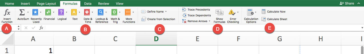
A. The Insert Function button is useful for those who don’t know all the shorthand. This brings up a side Formula Builder section that describes each function, and you can select the one you want to use.
B. These buttons divide all the functions by category.
- AutoSum works the same as it does in the Home tab.
- Recently Used is helpful for bringing up frequently used formulas to save time looking through menus.
- Financial includes everything related to currency, values, depreciation, yield, rate, and more.
- Logical includes conditional functions, like “IF X THEN Y.”
- Text functions help clean, regulate, and analyze plain text cells, such as displaying the character count of a cell (helpful for Twitter posts), combining two different rows via Concatenate, or pulling out numerical values from text entries that aren’t formatted correctly.
- Date & Time functions help make meaning out of time-formatted cells, and include entries like “TODAY,” which enters the current date.
- Lookup & Reference functions help pull information from different parts of your workbook to save you the trouble of looking for them.
- Math & Trig functions are just what they sound like, involving every sort of math discipline you can imagine.
- More Functions includes Statistical and Engineering data.
C. This section contains tagging options. If there’s a range of cells or a table you frequently need to refer to in formulas, you can define its name and tag it here. For example, say you had a column that contained the entire list of products you sell. You could highlight the names in that list and Define Name as “ProductList.” Every time you want to refer to that column in a formula, you can simply type “ProductList” (rather than finding that collection of data again or memorizing their cell positions).
D. This contains error checking tools. With Trace Precedents and Trace Dependents, you can see which cells contain formulas that refer to a given cell and vice versa. Show Formulas reveals the formulas inside all cells, rather than their display values. Error Checking automatically finds broken links and other issues with your spreadsheet.
E. Should you have a large sheet with a massive series of interconnected formulas, tables and cells, you can use this section to trigger calculations, and also to choose which types of data don’t run. A good example is a mortgage or asset depreciation sheet.
The Data tab is for performing more complex data analysis than most beginners will need.
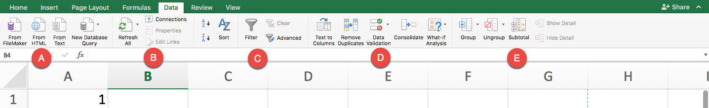
A. These are database import tools, allowing you to import data from any web, file, or server-based database.
B. This section helps you fix database connections, refresh data, and adjust properties.
C. These are Sort and Filter options similar to those for data you have within your sheet, applied to data feeds. They’re especially crucial here as a database is sure to have more data than you can or care to use.
D. These are data manipulation tools. You can take a single long string, like those separated by commas or spaces, and divide them into columns with Text to Columns. You can seek and remove duplicates, consolidate cells, and validate whether data meets certain criteria to assess its accuracy. What-if Analysis helps you fill in gaps with incomplete data using existing data and trends to determine likely outcomes for new scenarios.
E. These tools help you manage how much data you have to deal with at once and group them by whatever criteria you deem necessary. It’s similar to sorting, but you can choose any range of columns or rows and make them collapsible, each with their own label. Use Subtotal to create automatic calculations along a data set by different categories, which is helpful for financial sheets.
The Review tab is part of the Ribbon that helps with sharing and accuracy checks.
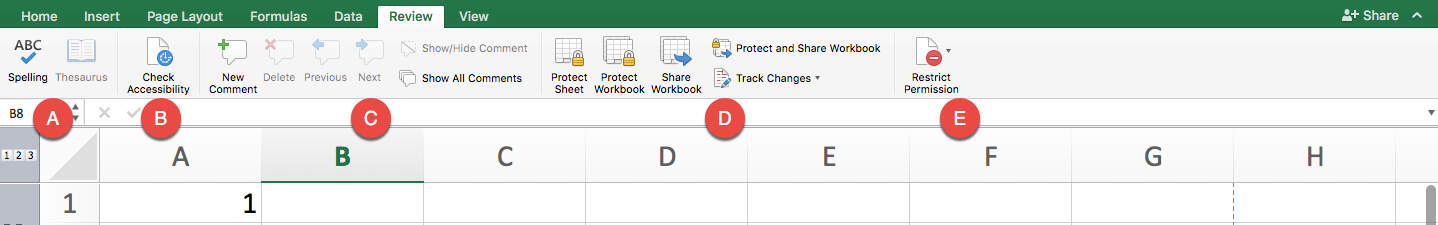
A. These are simple text-based checks (like in Word) that allow you to locate cells with spelling errors, or find more appropriate words via the Thesaurus.
B. Check Accessibility pulls up errors that can make it difficult to access the data in other programs, or just for reading purposes. It might find that your sheet is missing alt text, or that you’re using defaults for sheet names that can make navigation less intuitive.
C. The commenting tools allow collaborators to “talk” to each other within the sheet.
D. Protecting and sharing tools allow you to invite collaborators and restrict access to certain parts of the sheet. You can manually assign different levels of access — for example, you might allow a contractor to edit just the cells related to the hours they worked, but not the cells that calculate their pay. As with Word, sharing a sheet with Tracked Changes means you can see everything that’s been done to the sheet.
E. When you’ve shared a workbook, you can restrict permissions later on using this button and selecting individual contributors.
Use the tools in the View tab to change settings related to what you can see or do.
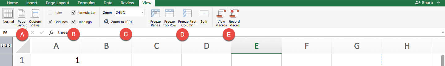
A. This is your basic view where you can see your default sheet view, how it’ll look when printing, and in custom ways you set yourself.
B. Use these buttons to choose whether you want to see the grids, headings, formula bar, and ruler.
C. This is another way to control zooming in and out of cells.
D. Freeze Pane controls are an important part of making a usable spreadsheet. Using these tools, you can freeze a number of rows and/or columns while you scroll around. For example, if the first row had all your column headings and remained frozen, you’ll always know which column you are looking at as you scroll down.
E. Macros are a way of automating processes in Excel. It is far beyond Excel 101, however.
How to Create a Simple Budget Spreadsheet in Excel
Now that you’ve learned about the tools in Excel, let’s practice making our own spreadsheet from scratch. This guide will cover basics, with a few intermediate techniques to get you more comfortable with spreadsheets.
Step 1: Create a Workbook
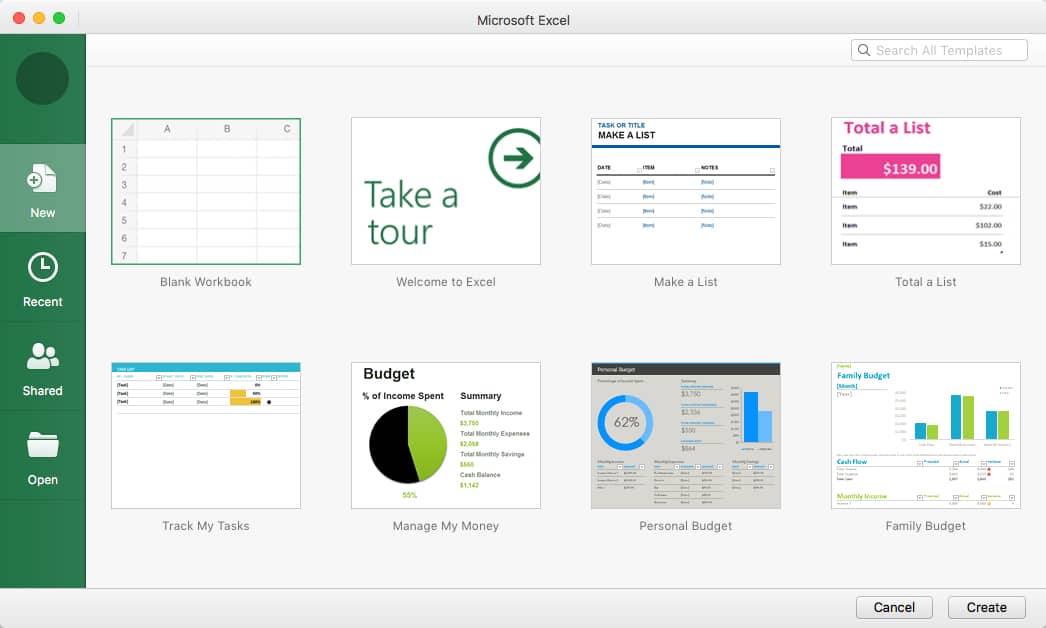
When you open Excel, you’ll be presented with a screen like this. Create a new workbook by clicking the New tab on the sidebar. The Recent tab below that will bring up any workbooks you’ve recently opened. Below that is the Shared tab, which shows workbooks that other Excel users have sent to you directly through the app (we won’t focus on that right now). The final tab is Open, which opens a file browser so you can select an existing workbook.
On the New tab, you can see a number of templates available, which can help you jump straight into making specific types of spreadsheets, like budgets and task lists. In this example, however, we’re going to build a spreadsheet from scratch. Click Blank Workbook on the top left corner, then click Create.
Step 2: Plan Your Needed Data
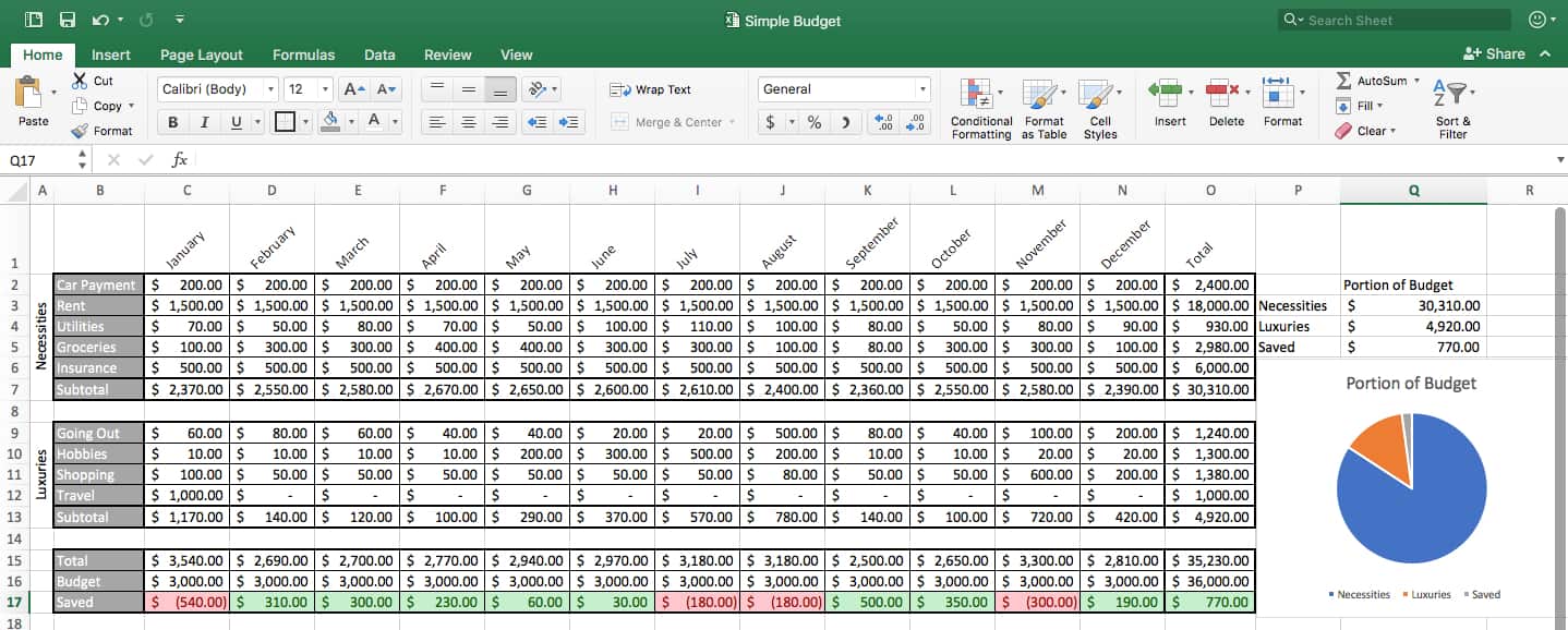
Before you can create any kind of spreadsheet, you need to plan what it’ll include so you can structure and format it accordingly. While it is possible to change the spreadsheet structure later on, the more data you’ve added, the more inconvenient it becomes. Plus, moving around entire rows and columns increases the chances of accidentally changing formulas. In this example, we’re making a monthly budget, so we’ll use a monthly time stamp. As we explored above, we can use other sheets in this workbook to track other time increments, like weeks or years. Of course we want to add all of our different expenses together, but we should also think of categories for comparison. We could have one for necessities, and one for luxuries. We’ll need subtotal rows, along with a comparison of budget to actual spending. At the end, we’ll also want to easily compare the different parts of the budget together.
Now we know the elements we need, and can organize them accordingly.
Step 3: Create Headings
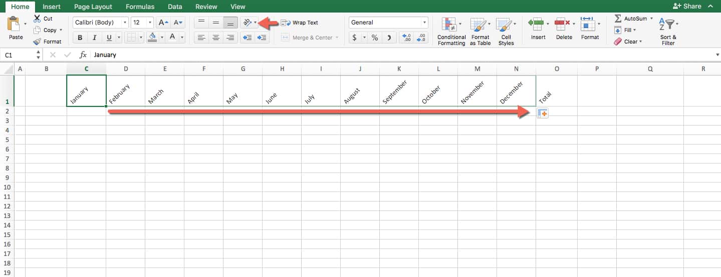
Since we know we want to compare month to month, we should use months as our column headings — horizontally is usually best for time comparison. Since we know we’ll also have categories of spending to label and sublabel, we should leave the A and B columns open, and start at cell C1.
Here’s a useful trick: if you type a number or timestamp with a logical next entry, you can click the lower right corner of that cell and drag in any direction to autofill the rest of the sequence as far as you want. For this example, after typing “January” in C1, you can drag it across to N1 and watch it fill in the rest of the months. To create the diagonal names in the screenshot, navigate to the Home tab and find and click the formatting option with a diagonal rising appearance. This makes the headings stand out without changing the column width. We’ll also need an area on the sheet where we can get row totals for more useful data, so create the heading Total in cell O1.
Step 4: Label the Rows
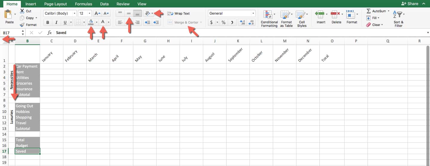
Create three blocks of entries on column B. Name the first block Necessities, which will include everything you see, and end with a subtotal. Name the second block Luxuries and include a few categories; also end with a subtotal. The last block will have our Total, the budget to compare it to, and the difference between the two, which we’ll call Saved (this amount represents the difference between the expected and actual spent). To makes them stand out, use the Paint Bucket tool and select a color (grey in this example).
For column A, we’ll create labels that clearly line up with our grey blocks, and position the writing vertically so it doesn’t take too much space. To make the width of the column smaller, grab the right edge of the A column and drag it to the left. To combine all the cells for our category labels, highlight A2 through A7, and Merge & Center. To get the writing vertical, navigate to the Home tab, find the formatting option and click vertical writing. Finally, choose the height alignment as centered so the vertical text will appear in the middle. Repeat this with cells A9 through A13.
Step 5: Add Boundaries
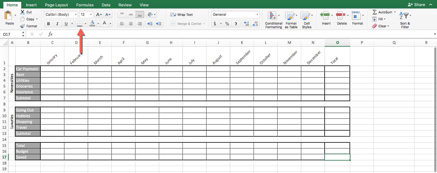
Add boundaries to the spreadsheet using the icon in the above graphic. Select each collection of cells, and don’t adjust the spaces between the grey block groupings. Click All Borders to draw distinct grids. Now, make the outer boundary of each block thicker by selecting the entire area and choosing Thick Box Border. Finally, do the same around the inner row of each box labeled Subtotal, to make these visually distinct. Apply a Thick Box Border to Column O, Total, and leave spaces between each row grouping. All of this improves spreadsheet readability.
Step 6: Create a Results Table
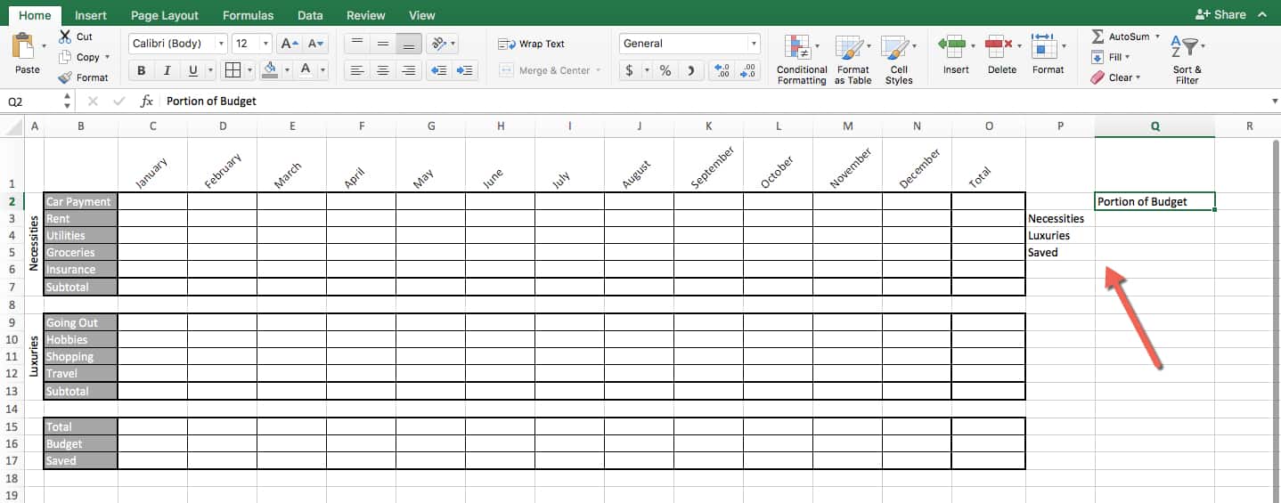
Use the side of your nicely-formatted spreadsheet to create the outlines of a simple table which will contain your main results. This information will assist you in creating a chart, later. Give it an appropriate label, and label its rows for the total from Necessities, the total from Luxuries, and the total Saved for the year.
Step 7: Format and Write Formulas
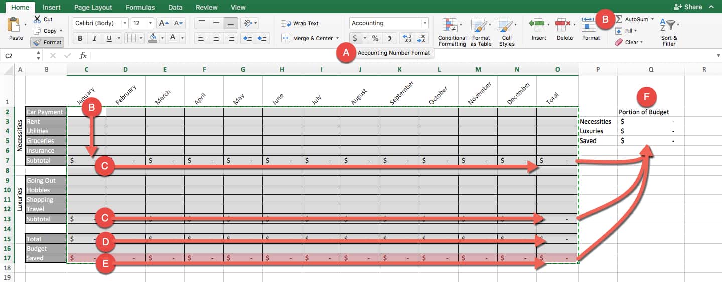
This is where the spreadsheet gets a lot more powerful. It involves a series of steps:
A. First, select every cell that will contain a number, underneath columns C through O, and also in the table for Portion of Budget. Now click the “$” on the keyboard to format the cells with the standard dollar format with two decimals for cents.
B. Select cells C2 through C7 and click AutoSum. This creates a formula that adds everything in this column, and places the sum into C7 (the last selected cell).
C. Use your cursor to grab the bottom right corner of cell C7, and drag it to the right toward column O. This will duplicate your formula down the entire Subtotal row. This means that while C7 = sum of C2 through C6, D7 = sum of D2 through D6, and so on. Repeat the process for Luxuries.
D. For the Total, Budget, and Saved area, the process is a little different. Click cell C15, and enter this formula: =C7+C13. This totals the two subtotals. Like you did with the other formulas, drag and duplicate it across to column O.
F. Click cell C17, and input this formula: =C16-C15. This will make the Saved row equal to the difference between Budget and Total.
E. Finally, add formulas to each empty cell of your Portion of Budget table. Q3=O7, which will bring the yearly subtotal of all Necessities items to the Necessities part of this table. Do the same for the Luxuries table annual subtotal and the Saved annual total.
Step 8: Script Conditional Formatting
Before entering data, there’s one more bit of set up: conditional formatting. To do this, click the drop down arrow on Conditional Formatting and click Manage Rules. Next, click + to add a rule, which takes you to a new popup menu. Click Style: Classic. Then choose Format only cells that contain, and click Cell Value greater than 0. Format this with a standard option, green fill with dark green text. Now you’ll be returned to the Manage Rules section, where you can select which range of cells it applies to. Choose C17 through O17 to have it affect the Saved row only.
Now repeat the steps, but this time Format only cells that contain the Cell Value equal to or less than 0. Use the standard option light red fill with dark red text, and apply it to the same range of cells.
Now you have a conditional format for all the final calculated Saved row entries. If it’s greater than 0, it gets marked green, and if it’s 0 or less, it gets marked red. When your data is entered, you can instantly see which months you saved money in, and which you didn’t.
Step 9: Enter Data and Watch the Calculations

First, enter an assumed budget, and copy it across the Budget row by dragging it from its bottom right corner. In this case, the assumed budget is $3,000.00.
Next, enter your data for each month of last year, totaled from receipts and bank statements, and categorized accordingly. Now for the magic of spreadsheets: as you enter each bit of data, you’ll see your Subtotals, Totals, Saved rows filling in, as well as the Portion of Budget table — all calculating and updating in real-time.
Step 10: Create a Pie Chart
Create a simple visualization. Select the entire Portion of Budget table, and then click the Insert tab on the Ribbon, and choose Pie Chart. Because of how the table is set up, the chart will be titled Portion of Budget, and each dollar amount will appear as a percent of the pie chart with the necessary label. Don’t forget to click Save on the top left of the Excel app.
Now you have an incredibly useful spreadsheet that tells you exactly how well you stuck to your budget each month while also getting a sense of where your money went last year overall. You can copy and use this spreadsheet year after year.
If you want more help getting started creating a budget, check out Top Excel Budget Templates.
Additionally, increase your speed with this complete list of keyboard shortcuts in Microsoft Excel.
How to Create a Spreadsheet in Word
Learn all the basics for making a spreadsheet with Microsoft Word. Word is the world’s most popular word processing application, featuring countless ways to format text-based documents, but also including simple tables and spreadsheets. Like Excel, the app comes as part of Microsoft Office and Office 365, and has versions for both PC and Mac. This tutorial uses the Microsoft Word version available in Office 365.
Unique Features of Word
In fact, Word isn’t really a spreadsheet app, but an app for typing and laying out text documents. It’s far easier to format sentences and paragraphs in Word than in the text boxes available in Excel, let alone inside cells. Because of this, Word can be used to create compelling reports or to insert semi-workable data into a text-heavy document, such as an article.
Word has two modes of spreadsheet creation: creating simple tables in the program itself, or inserting sheets and charts from Excel.
Understanding the Word Interface
Unlike Excel, where everything in the Ribbon is vital to creating a spreadsheet, only a few items are relevant in Word. For starters, almost everything you need is in the Insert tab. Here are the relevant Insert tab tools:
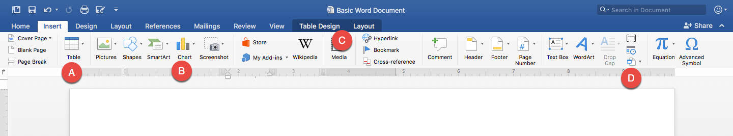
A. Table: Click this button to create basic tables in a few ways. When you click Table, a grid appears that you can hover over and click to choose the number of vertical and horizontal cells you want for your spreadsheet. If you click Insert Table, you get a pop-up window that lets you specify the spreadsheet’s dimensions by typing the number of rows and columns for the table, as well as setting the width of cells. Lastly, you can select Draw Table to drag and create as many cells as you like. Despite how simple it seems, Draw Table isn’t actually the best or easiest way to create a spreadsheet in Word.
B. Chart: A drop-down menu appears when you click this button that has the same types and styles of charts — and even the same interface — as Excel. You’ll see scatter plots, pie charts, line graphs, and more.
C. Table Design and Layout: When you click on any table in your Word document, two additional tabs appear in the center of the Ribbon — Table Design and Layout. Both tabs work only for tables, and contain further Ribbon menus explained below.
D. Object: You can bring Excel elements directly into your Word document. Either insert a Microsoft Excel Chart or a Microsoft Excel Worksheet. Selecting either of these options will open Excel so you can create and edit a fully functional spreadsheet that will then appear as-is in the Word document. These spreadsheets and charts behave like images in Word, so you can move them around and resize them, and even double-click them to open up Excel and update their data.
You can also insert an existing Excel file. To do this, click From File, then navigate to the location of the Excel file and open it. Initially, only the primary sheet appears, but double-click it to allow anyone to access the whole workbook, unless you protect it.
Let’s focus on the Table Design tab. These options are only for tables created within Word, not those imported from Excel.
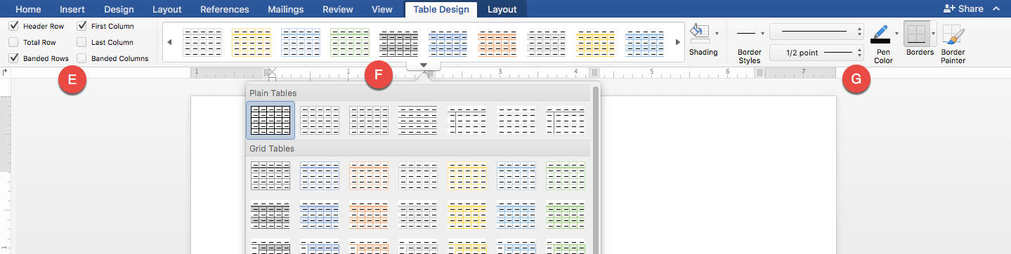
E. Use these toggles to choose certain table layout elements such as column, row, or header color.
F. These are style presents very similar to table styles in Excel, with a wide variety of colors and varieties. Plus, with the Paint Bucket icon, you can customize the shading rather than choosing one from the dropdown menu.
G. These tools let you design the borders of each individual cell, and the entire table. You can choose thickness, color, and type of line (dotted, straight, wavy, etc).
Next, let’s look at the Layout tab. Again, this only works for tables created in Word.
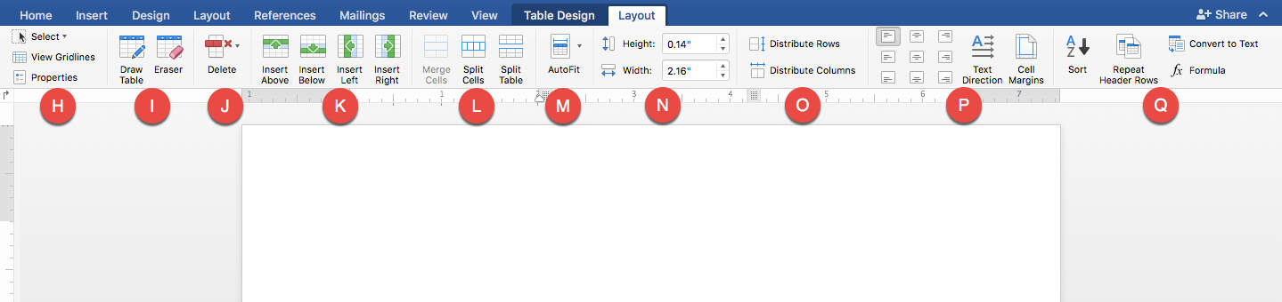
H. Use these tools to select rows, and choose whether or not to show the gridlines. You can also open up the Properties window and edit various elements, table alignment, or how the borders and shading appear.
I. This is another home for the Draw Table and Erase table tools. Use these tools to drag your mouse and draw each cell and erase them, one side at a time.
J. These are tools for deleting rows, columns, or entire tables. You can also do this by highlighting a cell, right-clicking, and selecting to delete these portions.
K. Insert rows or columns wherever you like in your table with these tools. Again, you can also access these tools by highlighting and right-clicking different parts of the table.
L. These tools let you change the organization of your table. You can merge and unmerge cells, like in Excel. This is a helpful feature for creating headers or spacing in your table. You can also split the table between any two rows.
M. Perform Autofit to automatically fit your table into the Word document’s space, or to make all columns the same width.
N. Adjust the height and width of rows and columns numerically, rather than using drag and drop.
O. Use these tools to select multiple rows or columns, and evenly distribute them across the page to make your table look clean and professional.
P. The alignment tools help you specify how to align the contents of each cell (top left, bottom right, center, etc.).
can also choose if you want the text to be horizontal or vertical.
R. Here is where basic spreadsheet functions live, and they aren’t nearly as robust as what you’d find in Excel. Sort works the same way, allowing you to select several rows in a column and use them to alphabetize the table. Convert to Text lets you select any number of cells and put them in text value without a table, separated by commas or spaces. This can be helpful for editing contents in paragraph form later, or importing data into other applications.
Finally, there are the functions. Word tables have 18 core functions that are mostly math with a couple logical IF and THEN functions. Calling cells in formulas is also somewhat more difficult in Word. If you have a single row table, then every cell will be row 1 — A1, B1, C1, etc. However, these aren’t labeled, so you have to count over, or just memorize them. You can also call by position: if you want to know the sum of all cells in a column and put it in the last cell, select the last cell, and make the formula “=SUM (ABOVE).” Likewise, use RIGHT, LEFT, or BELOW to call everything in those directions.
The other relevant item to spreadsheets that can be created in Word is the chart function. In the Insert tab, click the insert Chart button to access this feature. Once you choose a style, it will open Excel so you can edit the chart data. The functionality works exactly the same as in the Excel tutorial above. However, once the chart is in Word, two new tabs in the Ribbon, in place of Table Design and Layout. They become Chart Design and Format.
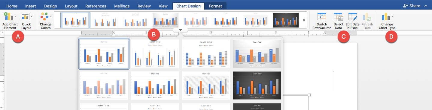
A. Use these tools to add extra important elements to your chart, either individually with Add Chart Element, or all at once using the helpful presets with Quick Layout.
B. Use these tools to adjust the style of your chart without changing its layout too much. You can adjust colors, drop shadows, background, and more.
C. Manipulate data in the chart with this set of tools. Switch Row/Column lets you change the X-Y-axes of your chart. Select Data takes you back into your Excel session to choose data set you want represented in the chart. Edit Data in Excel allows you to change anything you like about the data in Excel. You can also go into Excel by double-clicking your chart. When you return to Word, click Refresh Data to update your chart to reflect any changes made to the data in Excel.
D. Change Chart Type allows you to switch from a pie chart to a line graph and so on, using the same set of data.
Now look at the Format tab.
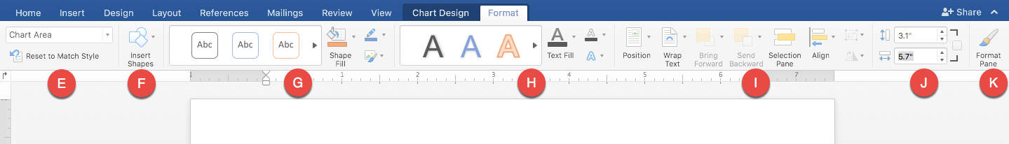
E. The selector tool lets you choose which part of the chart you’d like to edit so you don’t accidentally click elsewhere. You can select the Plot Area where the graph is stored, the Chart Area where all the axis labels exist, or any other element.
F. Use this to insert shapes into your chart, just like inserting any other object into Word.
G. Use these tools to color every element on your chart, which can include how you want to fill in lines, the text color, and more.
H. These are all your style options for text in your charts that handle adding WordArt, a fill color, and more.
I. The positioning tools work similarly to positioning other objects in Word. You can make the text wrap around the chart with Wrap Text, and place it behind or in front of any other element on the page.
J. Use these tools to numerically change the height and width of the entire chart. You can also adjust the chart’s height and width by grabbing the corner or side and adjusting it with your mouse.
K. This opens the Format Pane, which has some of the same tools found in the Ribbon, but they are larger and easier for some to access.
How to Import a Spreadsheet and Chart into Word from Excel
Now that you’ve learned about the spreadsheet tools in Word, you can practice a few different ways to import an existing spreadsheet into Word.
Step 1: Create a Word Document
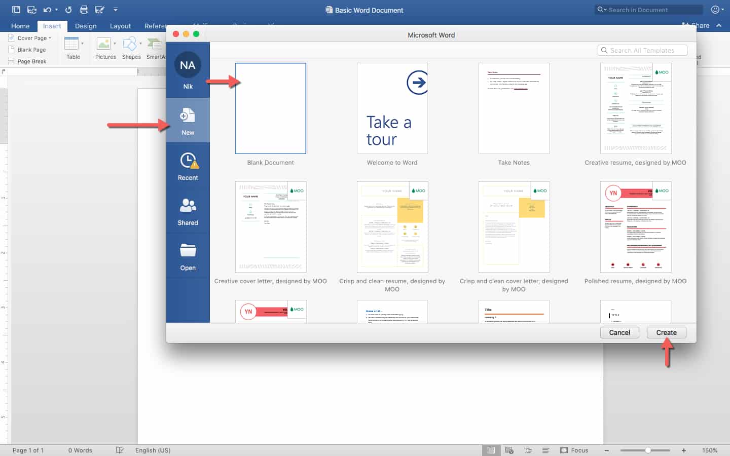
When you open Word, this screen appears. The New tab on the left side lets you create a new document, Recent surfaces recently opened documents, Shared shows documents that other Word users have sent to you, and Open opens a file browser for selecting an existing document.
On the New tab, you can see a number of templates which you can use to jump straight into making different types of documents like resumes, blogs, and research papers. Most don’t relate to spreadsheets at all, so click Blank Document on the top left corner, then click Create.
Step 2: Save Your Document
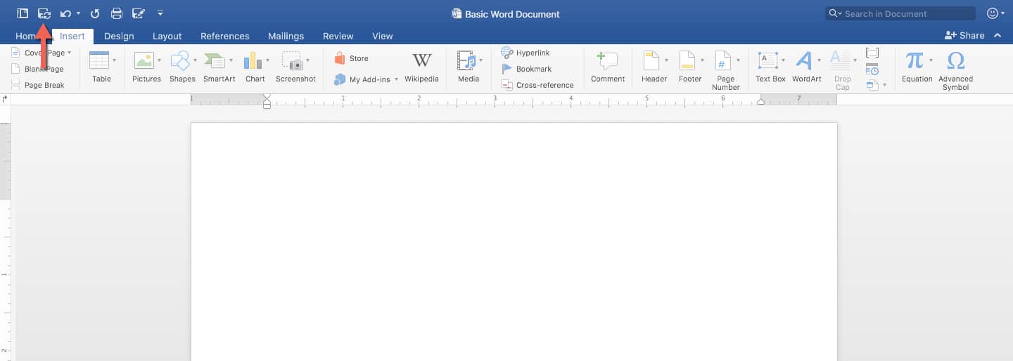
Once your document is created, save it by clicking the save icon shown above, and select a location to save it. Give it a name relevant to its purpose, so it’s easy to find.
Step 3: Import an Excel Workbook into Your Document
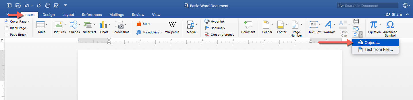
Go to the Insert tab, and click Object.
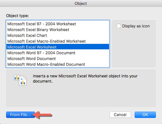
When the Insert Object popup window appears, click Microsoft Excel Worksheet, and then click From File. This opens a file browser window, where you can select the Simple Budget spreadsheet you created earlier, for instance. Open it.
Step 4: Resize Spreadsheet to Fit
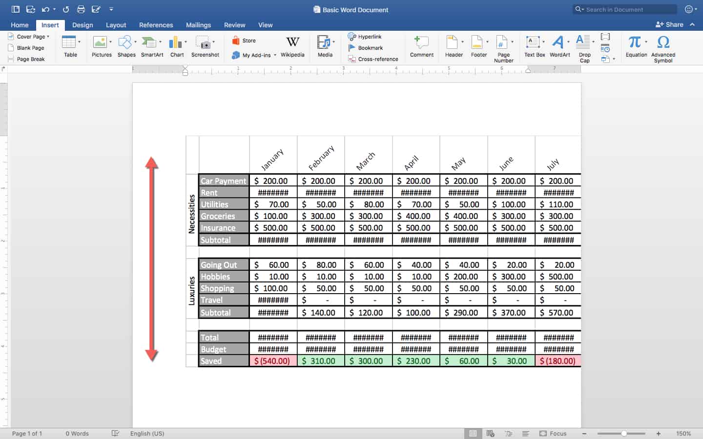
A spreadsheet as large as the one we created is too large for a standard Word document at its normal size. To shrink it, click once on the imported spreadsheet, and hold down the Shift key. While pressing Shift, select a corner of the spreadsheet and drag it towards the center of the object a few times. It’s important to note that spreadsheets behave like a regular picture or object in Word, so you can drag them around and change their size as you like. Feel free to add text below the spreadsheet, as well.
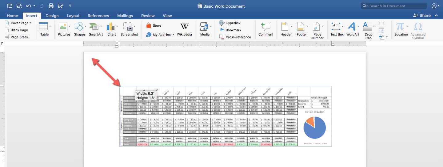
Regardless of the spreadsheet’s size, you cannot interact with the data within Word. However, all of your formulas and formatting will remain intact. You can still work with the rest of the document, typing words and inserting pictures around the spreadsheet.
Step 5: Edit the Data in Excel
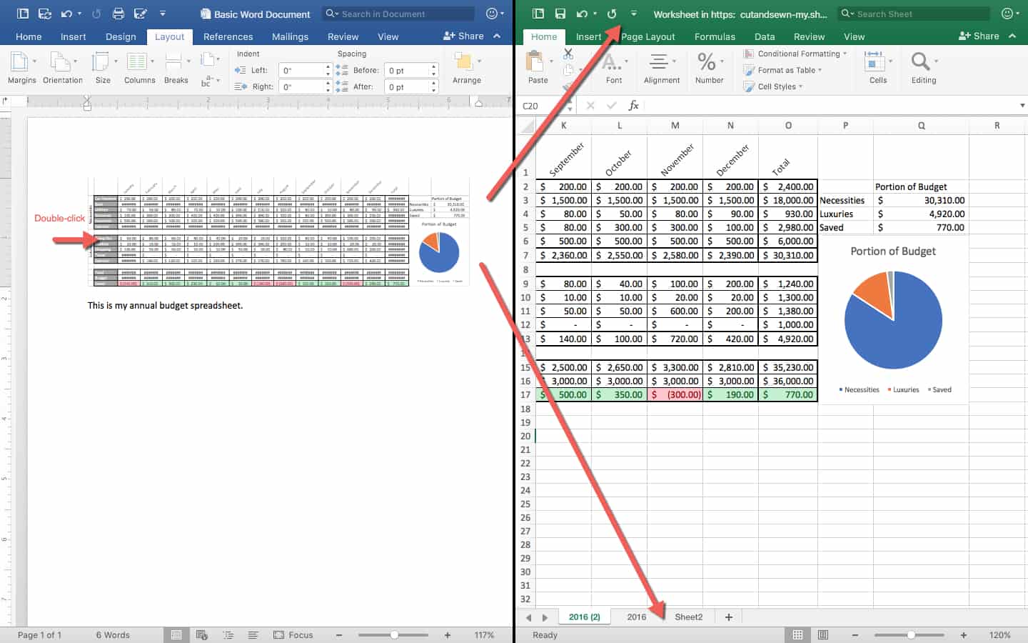
To edit the data, double-click the spreadsheet to open the spreadsheet in a new Excel window. Here, you can edit any data. It updates in real-time, meaning that as soon as you make the change in Excel, the change will be reflected in Word. In this way, you can bring fully-functional spreadsheets straight into Word.
Note: When you double-click on an inserted object like an Excel workbook, you have access to the entire workbook, not just the first sheet which appears as an object in Word. If you are sharing a document like this with someone and don’t want them to access other sheets, make sure to enable Protect Sheet in Excel.
How to Copy an Excel Spreadsheet and Chart Into Word
The newer version of Word lets you simply copy and paste cells and other Excel elements from an Excel workbook into a Word document. Here’s how to do it:
Step 1: Open Your Excel File
Open the Simple Budget workbook that contains your table, chart, and spreadsheet in Excel.
Step 2: Select and Copy a Range of Cells, a Table, or a Chart
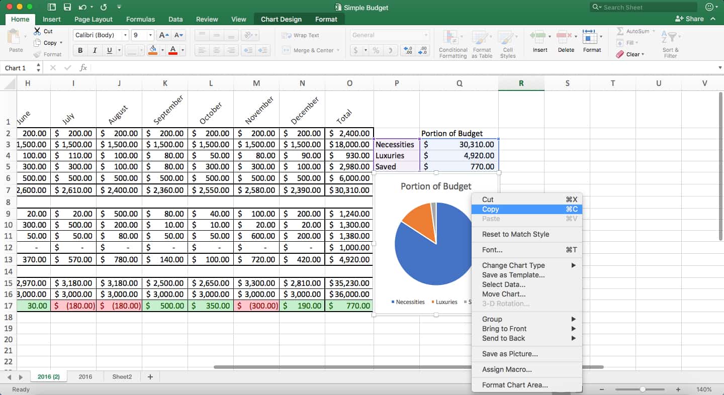
Highlight cells in the budget spreadsheet, then press Ctrl+C to copy the data. Alternatively, you can single-click the Portion of Budget chart, and press Ctrl+C to copy it.
Step 3: Open Your Word Document and Paste the Selected Cells or Chart
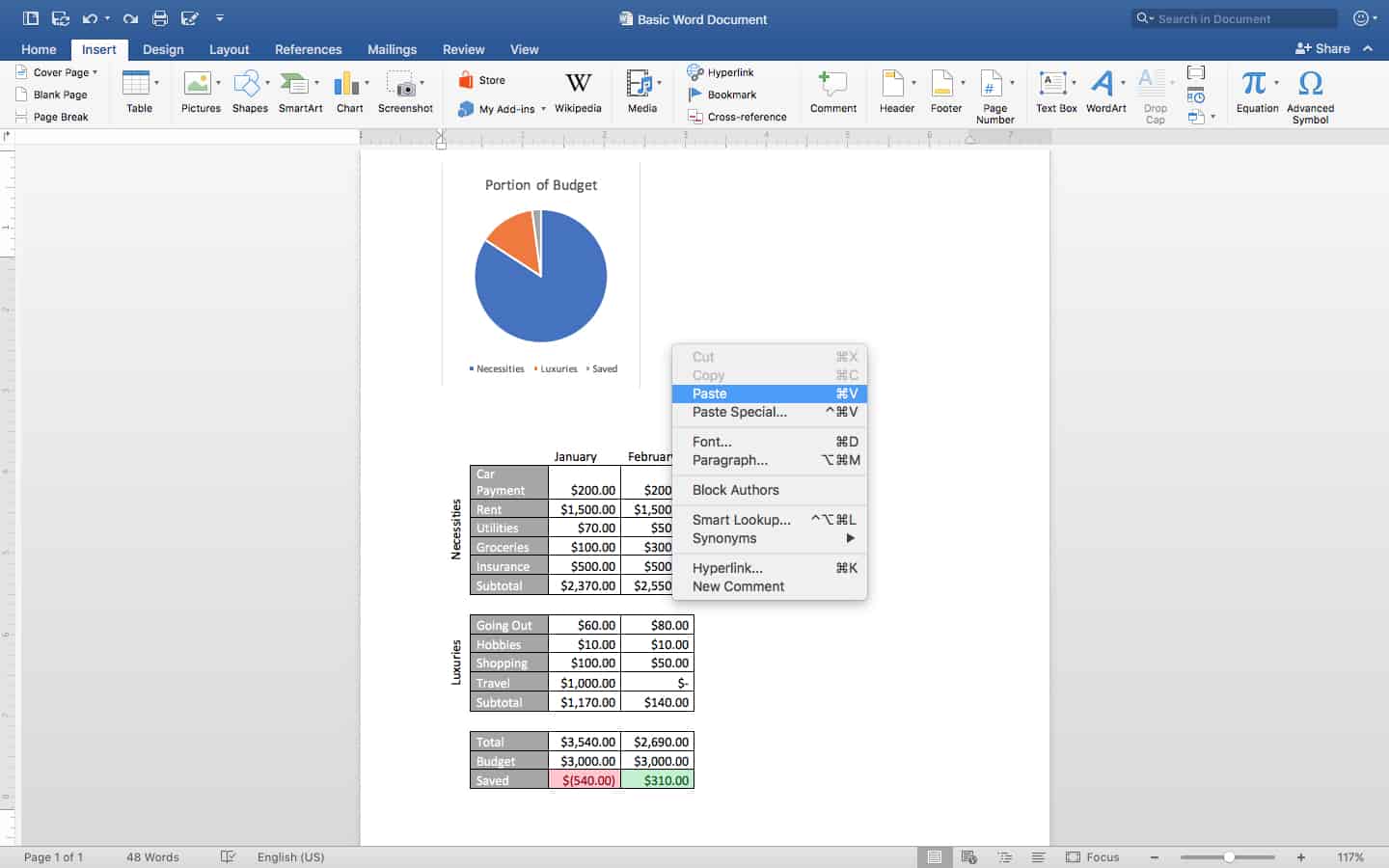
In your Word document, right-click on your mouse and click Paste to paste your chart and your selected Excel worksheet content into your Word document, one at a time. (Note that for this example, we aren’t copying the entire spreadsheet.) You’ll notice that some cell formatting is lost; this is because the data comes into Word and behaves like a table created in Word, rather than as an Excel spreadsheet.
Step 4: Format Your Data
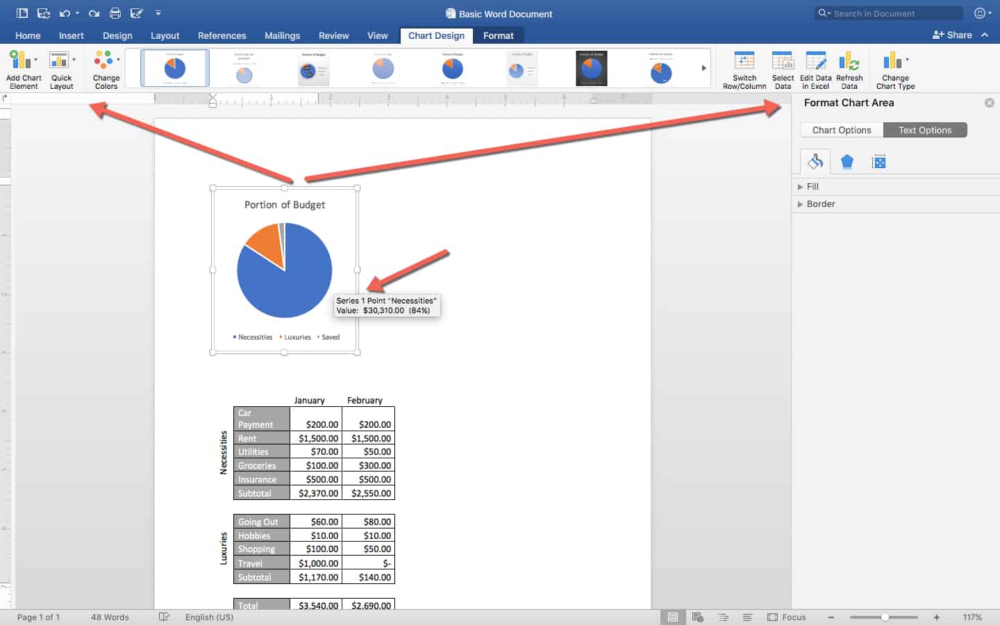
Charts in Word behave a lot like charts in Excel. When you single-click a chart to select it, it opens the Chart Design and Format tabs so you can manipulate information (for example, the design and layout). If you need to change some of the chart’s data, click Edit Data in Excel on the Ribbon. You can also hover over areas of this pie chart to surface additional information such as how many dollars the blue portion represents.
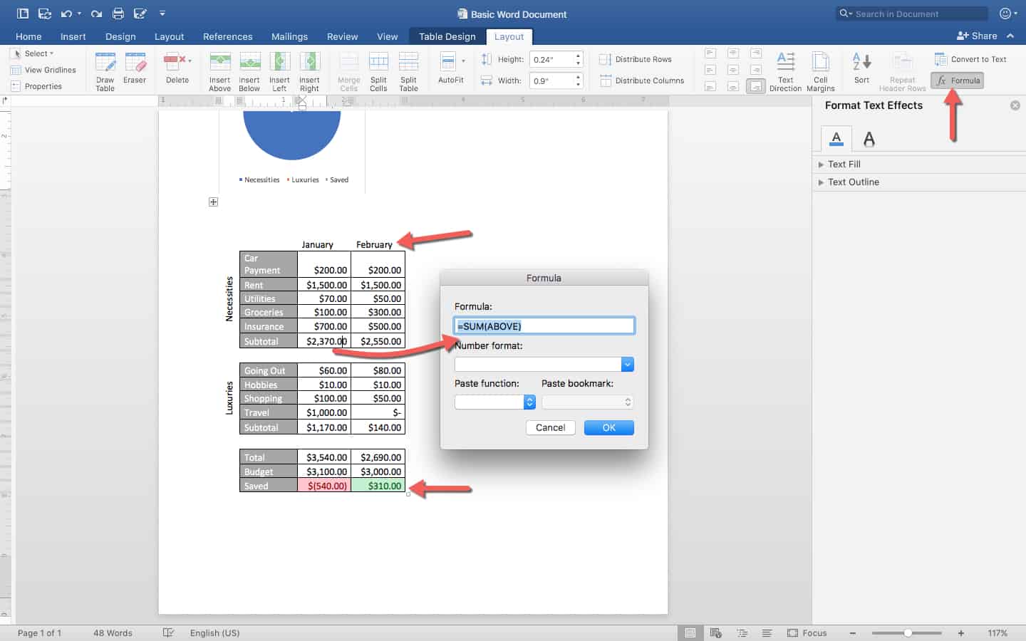
By contrast, spreadsheets and tables don’t behave the same in Word, because Word’s table abilities are much more limited. A lot of the formatting as is kept intact, but you lose almost all the formulas. For example, notice the months in the header are no longer angled 45 degrees upward. If you click on the Formula button while keeping your cursor in any cell, the formula that cell contains should appear. The January subtotal for Necessities claims to have the formula =SUM(ABOVE), meaning this cell is the sum of every cell with numbers above it. However, this isn’t true — editing the cells above won’t update the numbers. You can re-enter this formula, and it will insert the new sum, but it will treat the rest of the text inside this cell as just text, squeezing the new sum in with it.
The conclusion? Copying tables directly from Excel can be a quick way to get a visual table into Word. However, it is not useful if you need to update the data since it doesn’t retain formulas. Charts, however, are fine to copy and paste into Word, as they are still editable in Excel with their full functionality.
How to Create an Excel Spreadsheet and Chart Directly in Word
Step 1: Create and Save a Word Document
Create a Word document in the same way as above, and remember to save it.
Step 2: Insert New Excel Elements
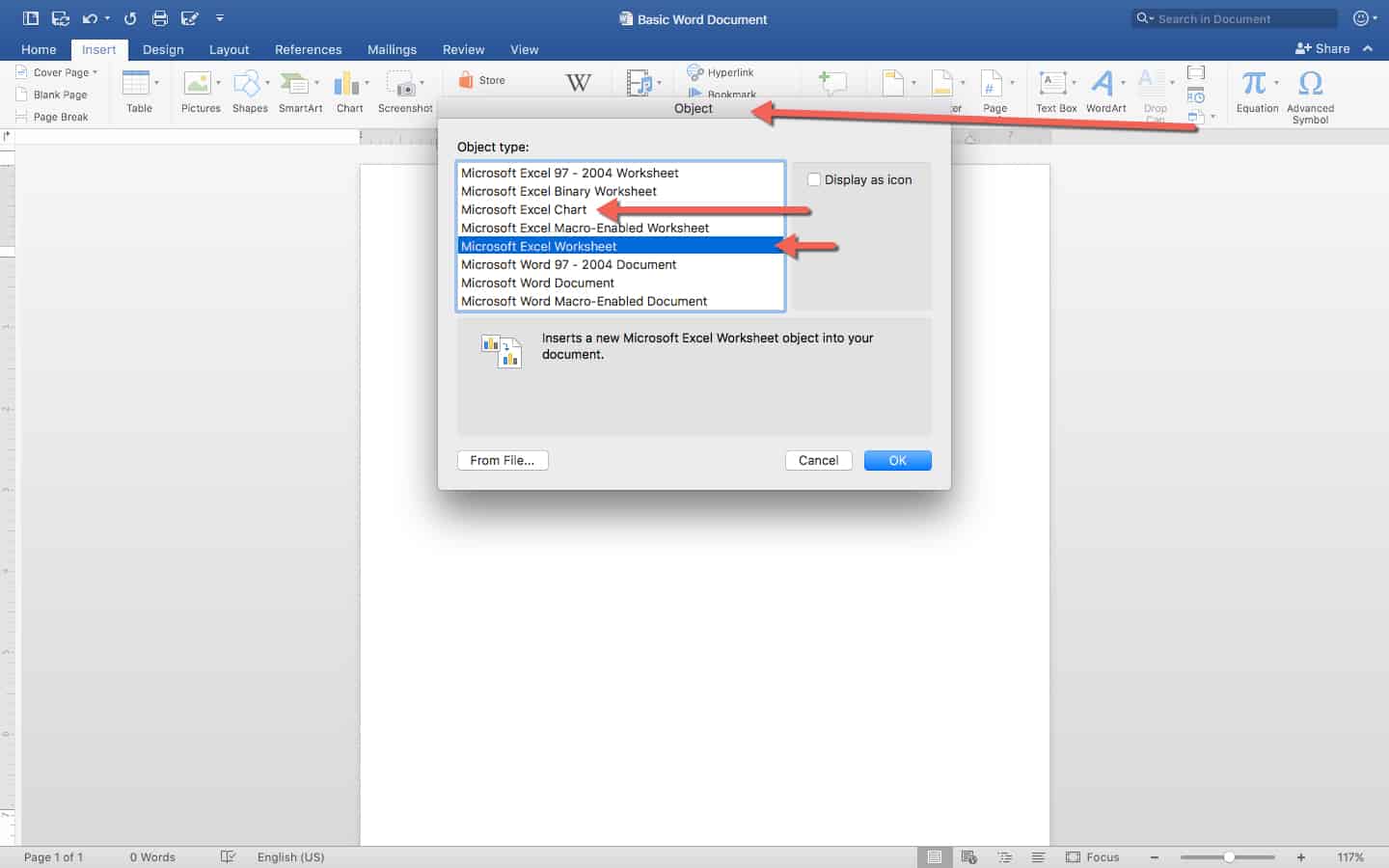
This time, open the Insert tab and go to Insert Object, then click either Microsoft Excel Chart to insert a chart, or Microsoft Excel Worksheet to insert a full worksheet. Click OK. Either option will open Excel.
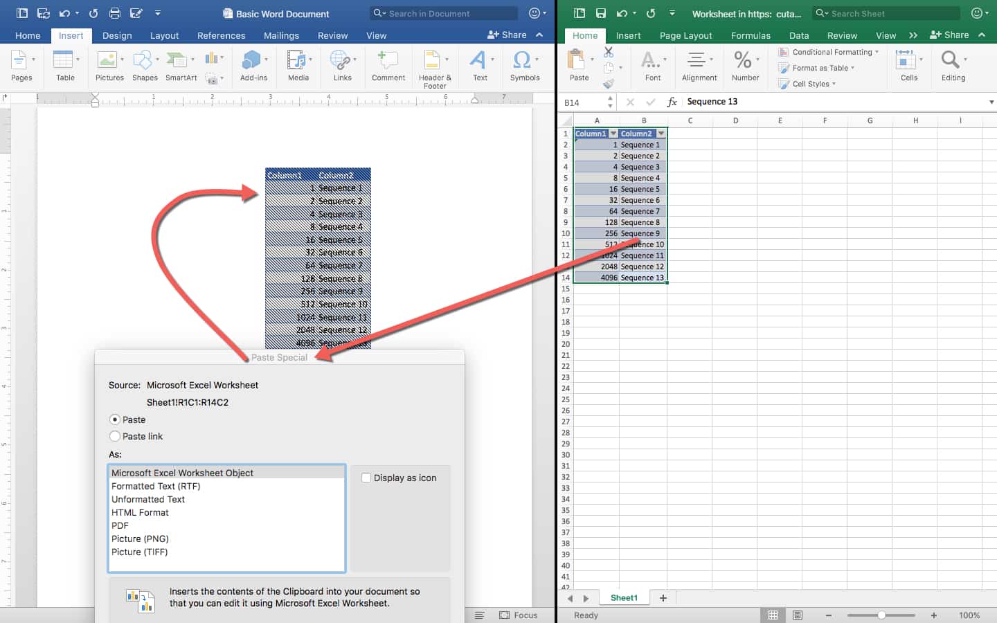
The Microsoft Excel Worksheet will open a blank Excel sheet. You can enter whatever information you want into it, following the same process as you used in the Excel tutorial above. Anything you change in Excel will immediately change in Word, as well, whether it’s spacing of cells, color and border formatting, or the formulas within them. You cannot change anything about the data in Word, and will again have to double-click the object to open Excel to make edits.
If you find you have extraneous cells, you can also double-click to open Excel, select the data you want, then right-click and select Copy. When you go back to Word, right-click and select Paste Special in the Edit menu, then click Microsoft Excel Worksheet Object. Delete the original object.
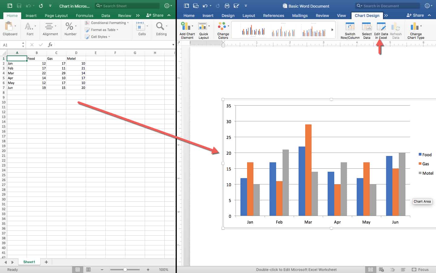
Charts will work as described in the previous section on copying Excel charts. Adding a chart will open an Excel file that has one sheet with the chart, and one with the data. Once you save the chart in your Word document, the data will stay in Excel with only one sheet, and the chart will appear in the Word document. You can change the data in Excel at any time by double-clicking the chart, and changing the styling of the chart in Word.
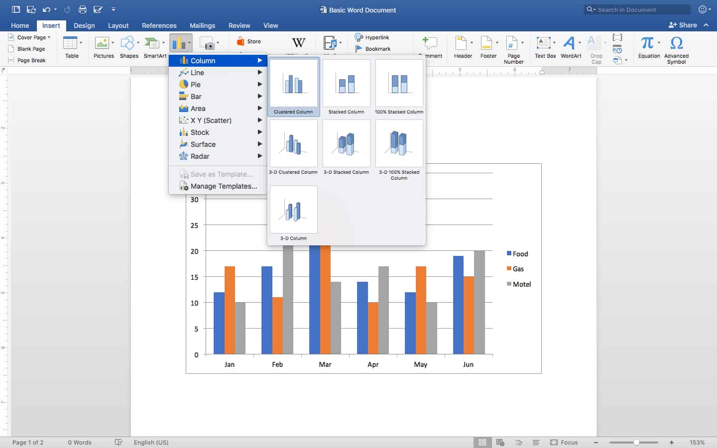
The other way to insert a chart into Word is to click the Insert tab, then click Chart, and select the type of chart and design you want. Then, you will be taken to Excel to enter your data from scratch, which will update your chart in Word.
Step 3: Change Alignment and Text Wrapping
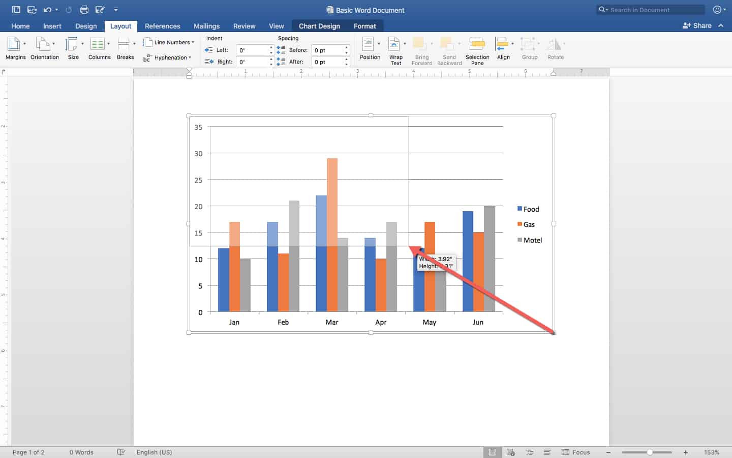
Now you’re going to learn how to adjust these elements in Word to make a working document. First, shrink the size of the chart by clicking the corner of the object and moving it inward. This action creates a more manageable size.
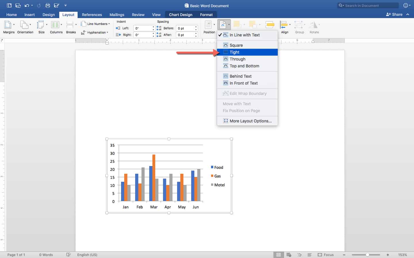
You’ll notice that it’s not very easy to move the chart around the document. Word automatically tries to force alignment on objects so that they don’t slide out of place and confuse users. To move your chart or table more freely, single-click on your table or chart, and click the Layout tab on the Ribbon. Select Wrap Text, and click Tight to drag-and-drop the object anywhere on the page.
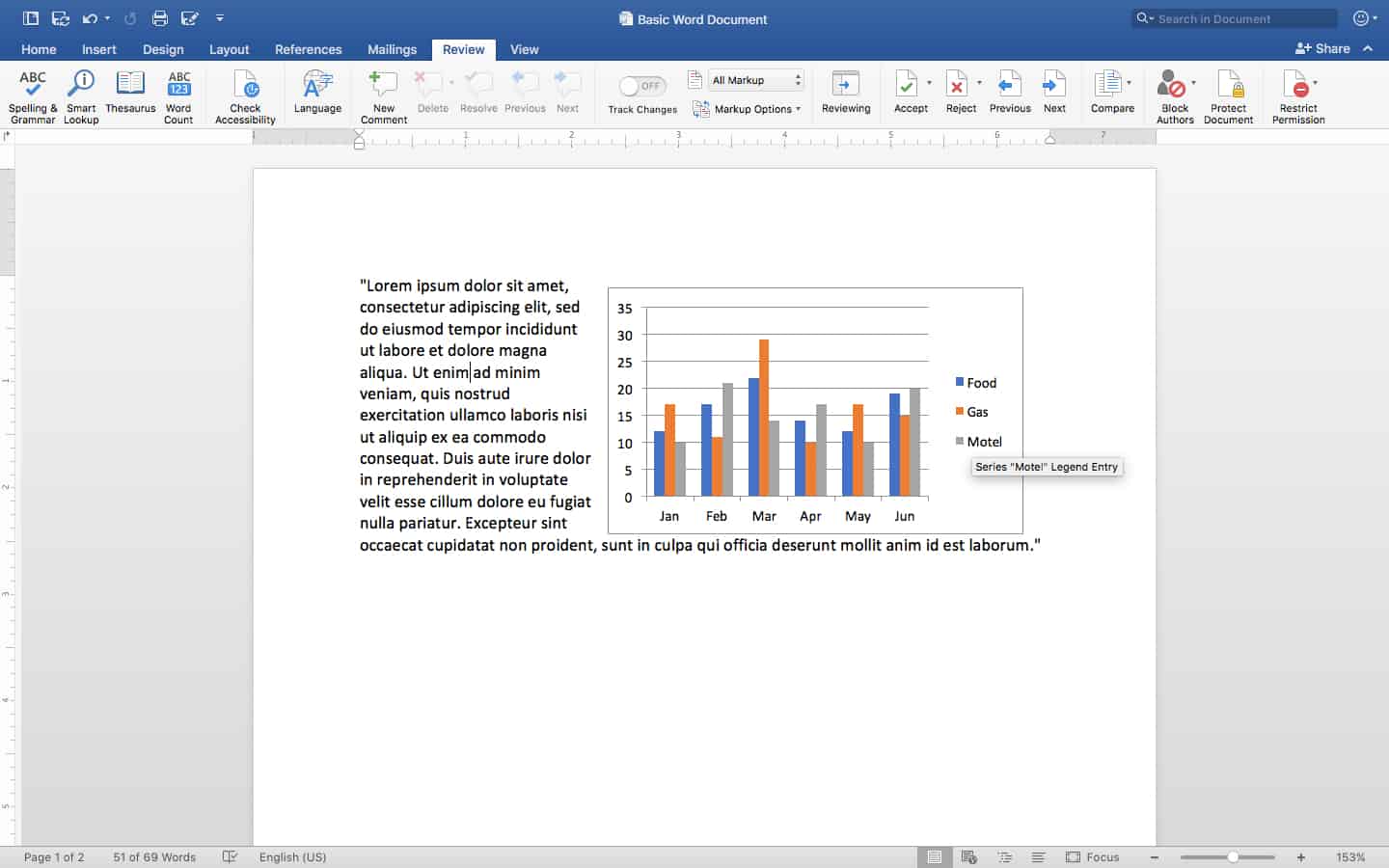
When you type words around the inserted chart, they won’t overlap or go behind the object, but instead neatly arrange around it (regardless of where you place it on the page).
How to Create a Pure Word Spreadsheet Table for Simple Scheduling
The final way to create spreadsheets in Word is to create a table from scratch. These tables are generally only capable of simple functions, so we’ll create a weekly schedule.
Step 1: Create and Save Your Word Document
Do this the same way as listed above.
Step 2: Insert a Table
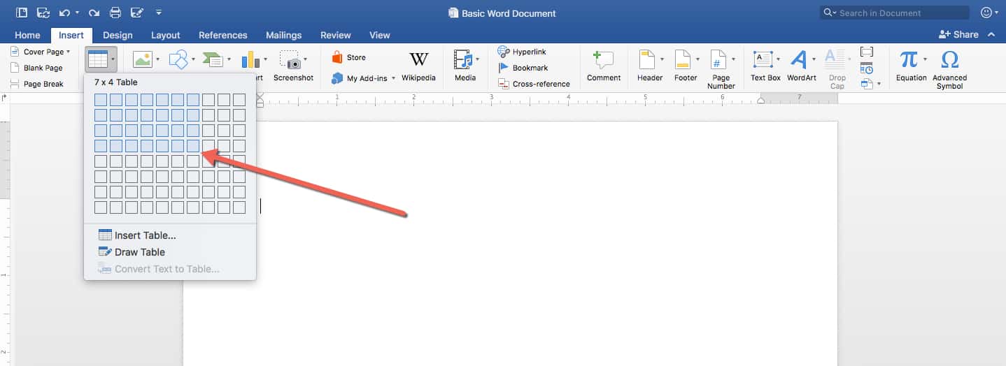
Click the Insert tab, and click Insert Table to see a grid. You can hover over the small squares to create a table of any height and width. Since we’re making a weekly schedule, we’ll do seven columns, and since we’ll have a header with three entries, four rows.
Step 3: Create Headers
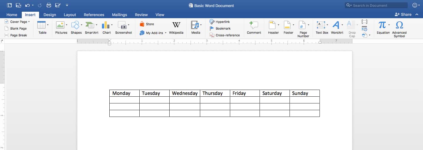
Now we have a blank table with a set amount of cells. The cursor appears in the first cell of top row. Start typing to create column headers. Don’t bother applying any styling yet. Also note that Word tables don’t have any of the Excel features that autofill data like days of the week, so you have to type each day manually.
Step 4: Enter the Data
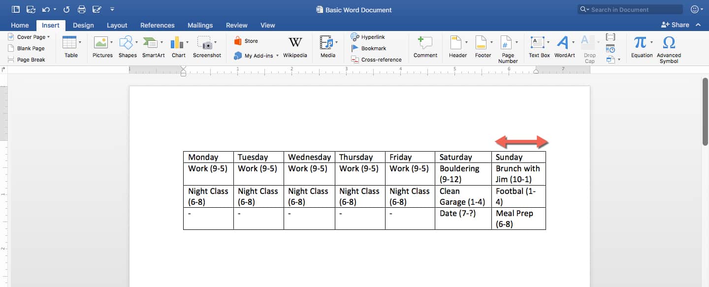
Enter your data for each day, consisting of your necessary tasks and the hours they require. For simplicity’s sake, our table will only include a few values.
Sometimes text might be longer than a cell, causing it to split into two lines. Change the width of the cells with longer content by grabbing the left or right edge of a cell, and dragging it as you see fit.
Step 5: Apply Styles
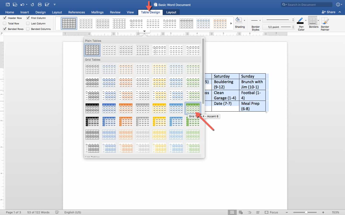
To make the schedule visually appealing, apply quick styling presets to it. Click the Home tab. Select your entire table, then choose a preset you like from the Ribbon. Since you have a heading row, make sure to choose a style that makes it visually distinct.
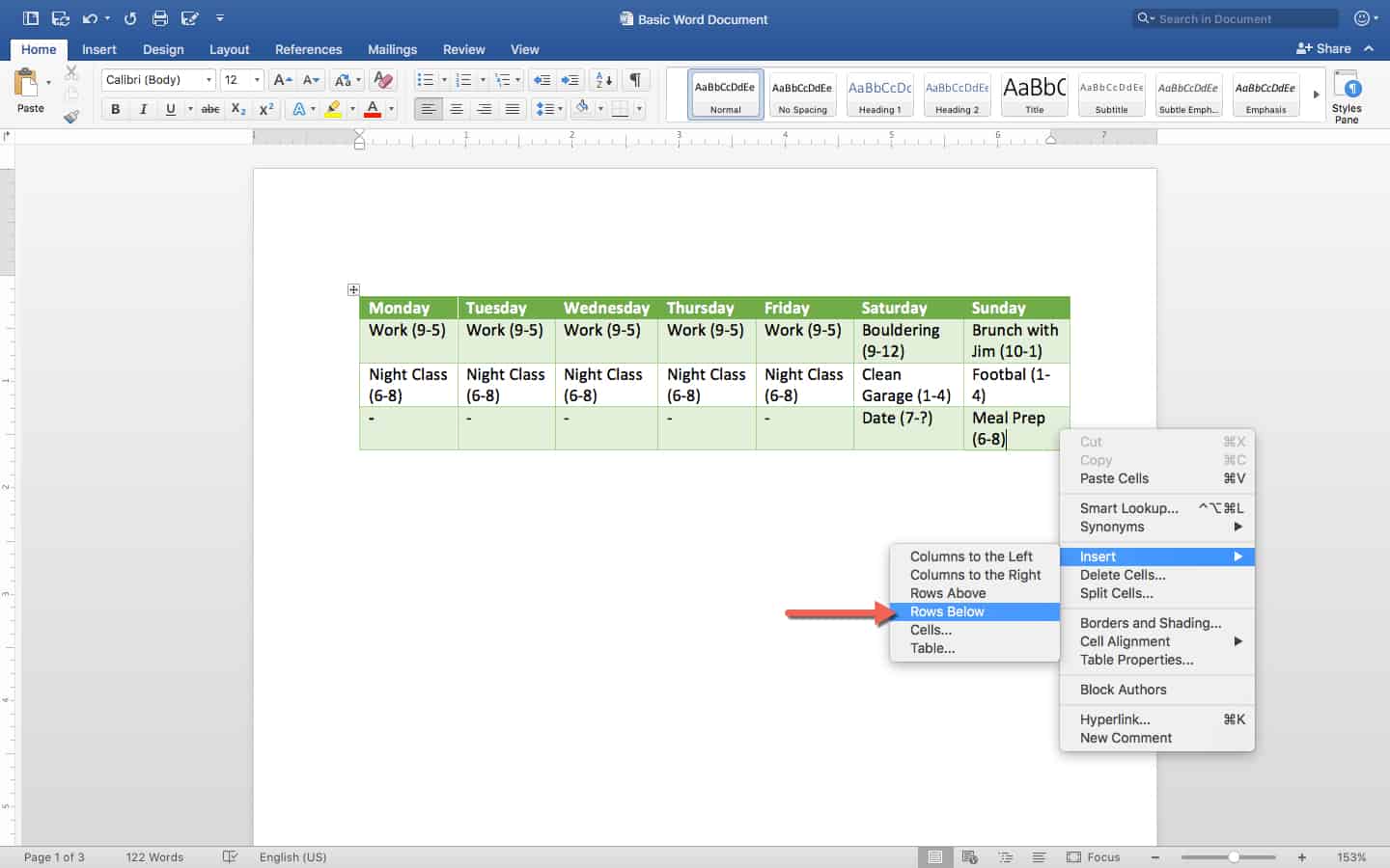
Now you have a simple, nicely-designed table you can use for day to day scheduling. To extend it and add more items to your to-do list, click a row and then right-click on your mouse and choose Insert: Rows Below.
See a complete list of keyboard shortcuts in Microsoft Word.
How to Make a Spreadsheet in Google Sheets
This section will cover all the basics for working with Google Sheets. Google Sheets is a spreadsheet app that lives in the cloud, meaning you never have to download anything, and you can update Sheets from any computer or smartphone. Most notably, it’s free — anyone with a Google/Gmail account can access all of its features.
Unique Features of Google Sheets
Google Sheets is not quite as robust as Excel in terms of functionality. It has fewer formula functions, a less accessible toolset, and you can’t set up any automation macros. What Google Sheets does have, however, is quite good for basic users: real-time collaboration abilities. This means that you can share a Sheet with other Google users, collaborate with them on the same spreadsheet, and see each other’s changes and comments instantly.
Google Sheet’s other unique feature is Explore, which lets you pull up instant insights about data, and also auto-generates charts, tables, and graphs to insert into a document.
Sheets integrates with all other Google products, allowing you to insert Google Forms data automatically. Sheets you create will be saved to your Google Drive account, and you can quickly insert any images you have in Google Photos.
Understanding Your Main Screen
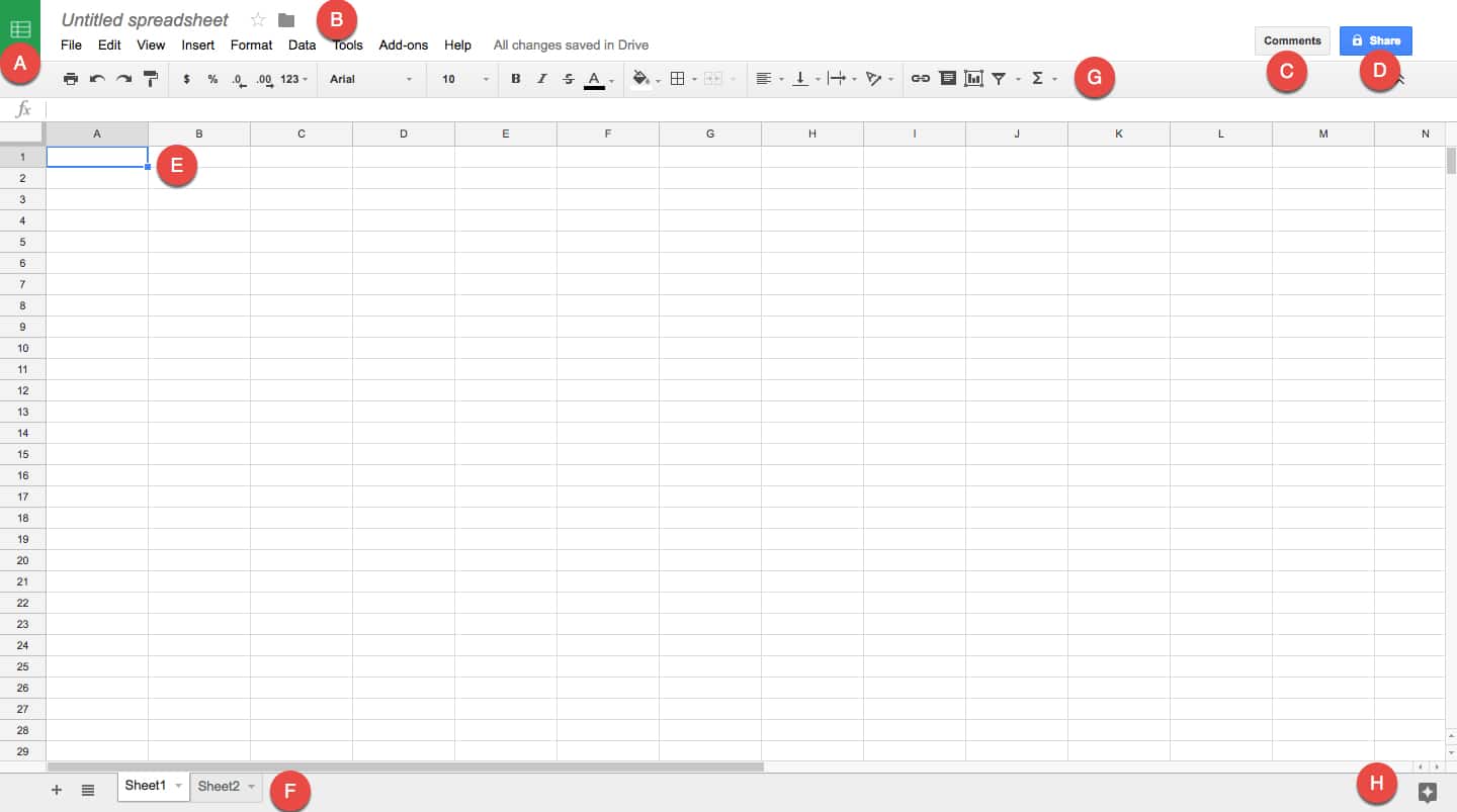
A. This takes you back to the Google Sheets hub page, which contains your most recent Google Sheets and a number of templates.
B. Use this area to name your Sheet. Click Untitled Spreadsheet and type a title for your sheet. Clicking the star lets you “favorite” this sheet so it’s easier to find. Clicking on the folder icon shows you where this file is located in your Google Drive, and allows you to move it.
C. All the icons along this grey section are your main toolbar. They include simple formatting options, alignment options, commenting, filtering, and some function tools. Below these tools is the Formula Bar, which works just like the Excel Formula Bar. You can enter and view different formulas for cells here.
D. The Comments button opens all comments and allows you to leave comments on the current cell or range of selected cells. It also lets you choose notifications settings: get notified every time you make a change made, every time any user makes a change, or never.
E. The Share button is essential to Google Sheet’s value proposition. When you click it, you can enter in the email addresses of everyone you want to receive the Sheet. Start typing the name of someone in your Google Contacts, and Sheets will recognize and autofill it. You can also choose the permission level of people you’re sharing with: either let them view it, let them view and comment, or let them view, comment on, and edit it. You can also lock down more permissions in Advanced Settings.
F. This is your workspace. It functions very similarly to Excel, with columns A-Z and beyond, and rows 1-any number you like. Each cross-section is a cell with a unique address, like A1 highlighted here. This is important for formulas.
G. Use these tabs to access the multiple sheets in one Google Sheets document. The tabs function exactly like Excel’s sheets, but you can color them to easily differentiate.
H. Hovering over this icon surfaces Explore. Clicking on this brings up a righthand pane that generates unique information about any selected group of cells, charts, or tables.
Navigating the Tools in Sheets
Unlike Microsoft products, Google doesn’t have a variable Ribbon of tools, just a series of drop-down menus with similar functions. This section will cover where to find all the spreadsheet tools in Google Sheets.
A. These are some basic functions, including the print tool, undo and redo, and the format paintbrush. Use these tools to take the color/style/attributes/formats of a selected cell and apply them to any other cells you highlight immediately afterwards.
B. Use these text formatting tools to turn number entries into percentages, or standard dollar formats like “$1.00.” Use the quick buttons in this area to add or remove a decimal place.
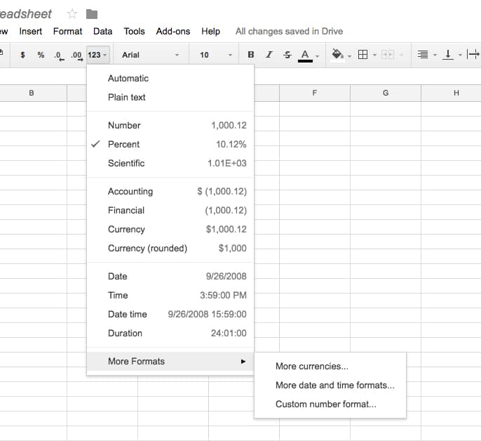
Click the drop down to see more currency, date and time formats, and other options hidden in another menu.
C. This is a standard font selector. Choose any built-in fonts to format the text in any cell.
D. A standard point-size selector for any characters you’re typing into a cell.
E. These are mostly standard style formatting tools for text, like bold, italics, and text color.
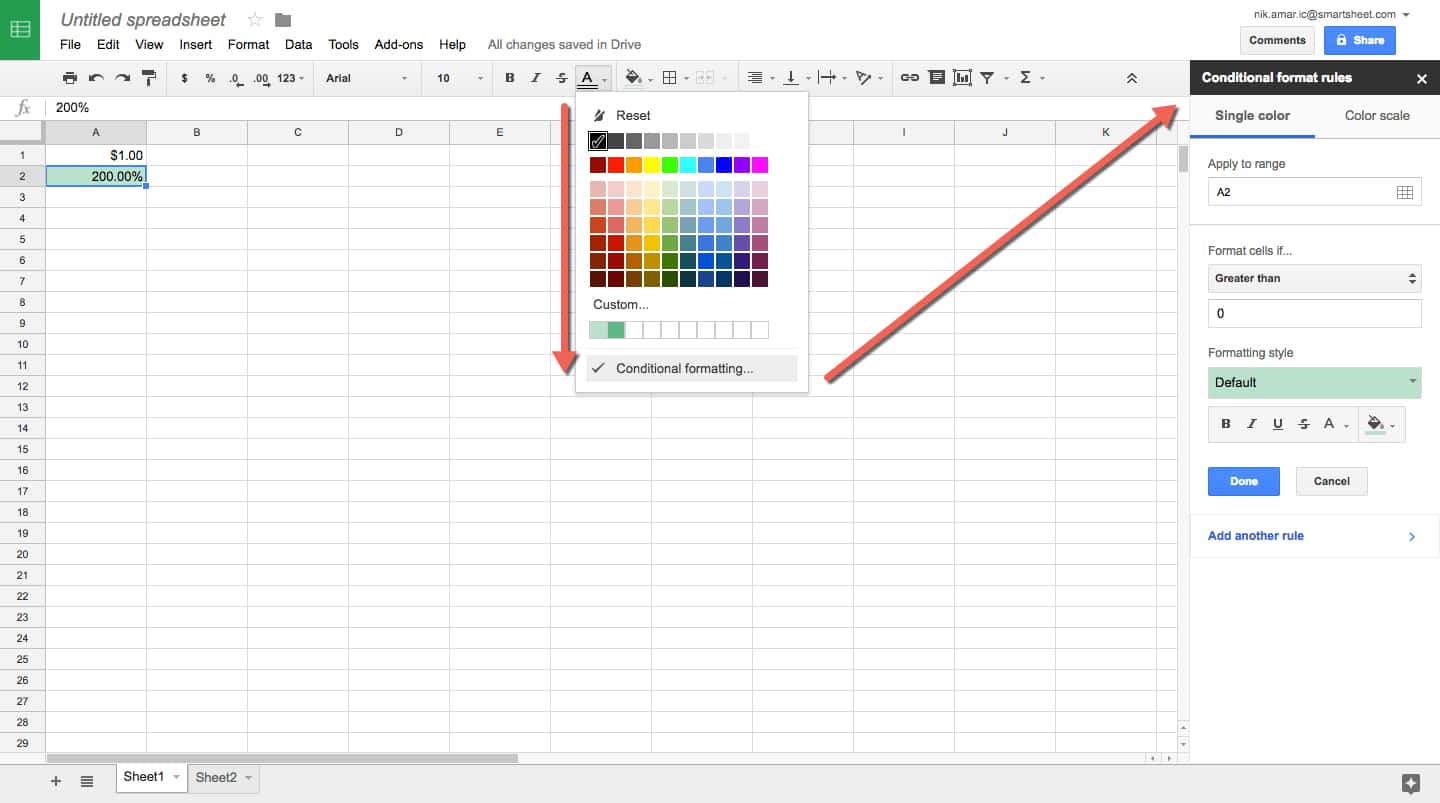
The text color selector is also where you’ll find the “conditional formatting” tools. These tools allow you to choose a range of cells and create if/then conditions to change their formatting (color, font, size, background color, cross-out, and more). You can add numerous rules to a single selection of cells so their format will reflect your chosen status at a glance.
F. This is where cell style formatting options live. You can also access conditional formatting tools in the paint bucket drop-down menu. Use these tools to either select or draw your cell borders, including thickness and style (dotted line, straight line, etc.). The last button here controls merge, and works just like it does in Excel and Word tables.
G. These are alignment tools. You can choose left, right, and center align, as well as top, bottom, and floating alignment in the cell. The third icon is Text Wrap, allowing text to either overflow into the next cell, wrap downwards and increase the height of your cell, or “clip” the text when it starts overflowing. (The text is still there, it’s just hidden.) The final button in this area lets you angle your text differently, like in Excel.
H. These are tools that work for higher-order purposes. The first lets you make a cell or range of cells link to a website or file. The second is your comment options — just highlight a range of cells and click it to comment. Others can reply to your comments, too.
Next is Insert Chart, which brings up a fairly robust popup window with numerous data visualization options. There are more types than found in Excel, but there are fewer styles of each. In addition to line, bar, and pie charts, there are maps that light up based on location data you include, org charts for companies, radar graphs, and Venn diagrams, to name a few.
The next icon is for sorting and filtering, which lets you insert filter menus on top of each column that you can update and change in real time.
The final icon is your primary formula drop-down menu. It only shows a few functions by default — SUM, AVERAGE, COUNT, MIN, MAX. The rest of the functions are hidden in More Functions, which brings up a new page that just has a list of functions. The Formula Bar also has an autocomplete feature: start typing “=” and a couple letters to reveal a list of functions with those letters for you to select and insert into the formula.
All the other tools are hidden in drop-down menus, which are covered below. File and Edit contain basic functions for downloading, sharing, undoing, and redoing. The Edit menu also has Find and Replace, which lets you scan the document for any cells containing your search criteria.
View Menu:
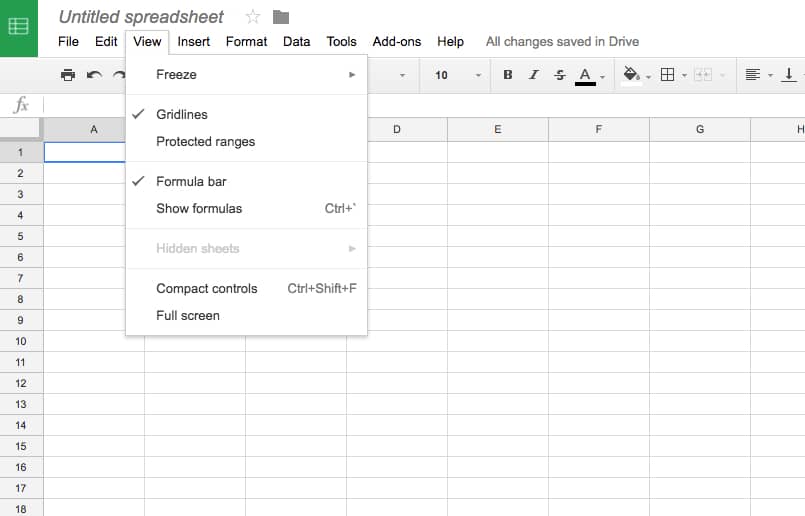
- Freeze: This submenu contains everything you need to freeze panes. You can freeze any number of columns and rows you like, so that necessary information stays put while you scroll around the screen. For example, if your first row has heading names for all the columns, you can see those headings no matter how far you scroll.
- Gridlines: This controls whether or not you see the grids on your worksheet. It might be necessary to remove them when printing, for example.
- Show Formulas: When you enter a formula into a cell, it will display however that formula resolves as a value. For example, if A1=1 and B1=2, and you made C1 have the formula “=A1+B1”, then it would show the value of 3. However, what the cell actually contains is its formula. Show Formulas displays the formula for all cells, rather than their value.
Insert Menu:
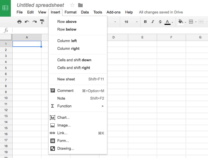
The first few parts of the menu let you insert columns, rows, and cells where you like, or add another sheet to the workbook. You can also add comments, charts, and functions.
- Note: Use notes to explain data and guide users, rather than as comments to be responded to. You can add a note to any cell or range of cells can be given a note.
- Image: Import an image into your Google Sheet from Google Photos, Google Drive, a website, or your computer.
- Form: Insert a Google Form into your sheet. This allows data collected from the form to appear as new rows in the sheet.
- Drawing: Google Drawings is a tool that lets you drag and drop shapes and colors to create simple infographics and diagrams. You can bring them into a sheet straight from that app.
Format Menu:
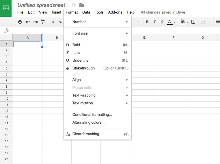
The Format menu consists of redundant tools that are also on the toolbar, but has two additional tools:
- Alternating Colors: A sidebar appears on the right side of the sheet that lets you build tables with alternating colors like in Excel. There are presets, some with a header color that is distinct from the rest, and it also allows you to build custom versions. Simply select your cells and apply it to them.
- Clear Formatting: Highlight cells and press this button to remove all formatting, leaving the cells bare with just their contents and/or values displayed.
Data Menu:
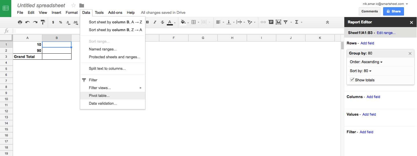
- Sorting: The sorting options are redundant with the sorting tools on the main toolbar. These add ranges that you can sort within.
- Protected Sheets and Ranges: This lets you choose certain cells or sheets that you want to prevent people from editing.
- PivotTable: These PivotTables work like they do in Excel: select a group of data with at least two columns, and create reports. The report editor appears on the side, letting you choose what data you want grouped in rows, columns, and what values and filters to use.
- Data Validation: For more complex sheets, this feature can find errors and missing data for you to correct.
Tools Menu:
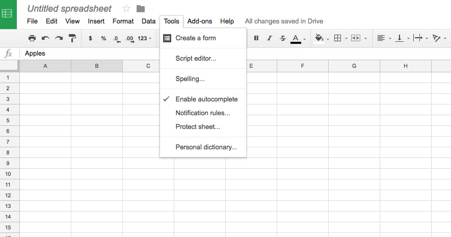
- Create a Form: This launches a Google Form creation window, automatically tied to your Google Sheet. When you embed this into websites or send through an email, all response data will feed into your sheet.
- Script Editor: This allows you to write custom functions and scripts to automate and extend the abilities of Google Sheets. This feature is for advanced users only.
- Enable Autocomplete: A useful setting that allows Google Sheets to use what it learns to fill-in information. It’s recommended to keep this on.
- Protect Sheet: This lets you password protect parts or all of your sheet so that only the right people you’ve shared it with can access it.
- Personal Dictionary: This is every word your Google Account has been told is a correctly-spelled word that doesn’t exist in its main dictionary.
Form Menu:
This menu just has some redundant features about Google Forms.
Add-Ons:
This menu has links to Google Sheets add-on marketplace. These are mostly unofficial extensions that different developers have created to make Google Sheets more useful. They don’t always work properly, and aren’t recommended for elementary users.
How to Create a Product Sales Tracker in Google Sheets
Now that you know about all the tools in Google Sheets, practice making your own spreadsheet from scratch. This guide will cover basics and some of the app’s unique features to quickly produce a great spreadsheet. For this example, we’ll build a more complex spreadsheet than we did in the previous two examples.
Step 1: Create a New Google Sheet
Start by opening Google Sheets. You can search for an existing sheet or open it within your Google or Gmail account, near your icon in the top right corner. The Grid Icon should list the Sheets app. Once you arrive on the main Google Sheets hub page, you’ll be able to see and search for any other spreadsheets you’ve created, and choose templates. Let’s start from scratch and click Blank.
Step 2: Plan Your Data
As with the Excel spreadsheet, you must plan out what data and analysis you need in order to correctly structure your spreadsheet. In this case, we’re making a spreadsheet that can track worldwide sales of different products with different prices and profitability. Since you have multiple products, you’ll need a reference table of pricing, cost, and profit. Then you’ll need a table where you can record every sale, including how many of each product the sale included, and the total profit from those sales. You also need to include calculations that remove different countries’ tax rates from your cost-based profit margin.
To help plan out things like this for your own situation, consider analytical goals. In this case, what information would a company selling products worldwide want to gain from a spreadsheet?
- Which product sold the most units?
- Which country netted the greatest profit?
- Which country had the greatest quantity of items sold?
- What was the total profit from sales worldwide?
Step 3: Create a Reference Table
A. Start by naming your spreadsheet. It’s best to be descriptive and unique, so you can easily search for it later with Google Drive’s search tool.
B. Create names for each column of the reference table. We’ll use Product, Price/Unit, Cost/Unit, and Profit/Unit.
C. The products will be A, B, and C. Add those letters to the cells A2, A3, and AC, respectively. They have variable prices, but all cost the same to produce, so each will have a different profit margin. To create this, click cell D2. Enter “=B2-C2” in the formula bar to calculate the profit of each unit. Then click the bottom right corner of the cell and drag it down to D4 to duplicate the formula for rows 3 and 4. Now you have the profit margin calculation for each product.
D. Finally, to keep it easy to view, apply some styling to the table. Just highlight the whole range of cells, then click the Format menu. From the drop-down, select Alternating Colors, which opens the sidebar menu where you can apply table styles. Select a preset that makes the header distinct. Click the X in the top right corner of the Alternating Colors sidebar to close it.
E. Enter amounts for Price/Unit and Cost/Unit.
Step 4: Create a Sales Tracker Layout
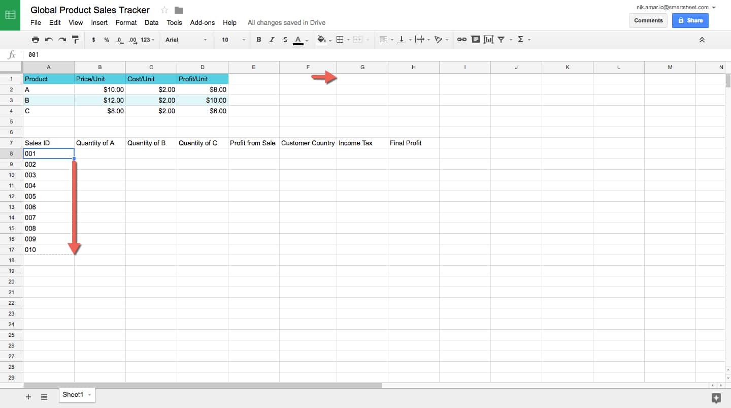
Let’s start laying out the sales tracker table. A company will likely track orders by the order in which they arrive, so click cell A7 and type “Sales ID.” Add order numbers to cells A8 through A17 under the Sales ID header. It’s also important to know how many of each product were sold, so make the next three columns product quantities for A, B, and C. To do this, type “Quantity of A” in cell 7B, “Quantity of B” in cell 7C, “Quantity of C” in cell 7D. Obviously, the company wants to know the profit from this individual sale, so type “Profit from Sale” in cell 7E.
The country of the buyer is also important for our analysis because for a real company that would affect the cost of doing business in the form of taxes, which would also reduce the final profit. You’ll need dedicated columns to track this information, so type “Customer country” in cell 7F, “Income Tax” in cell 7G, and “Final Profit” in cell 7H.
Also note that after entering our column headers, column F wasn’t wide enough for Customer Country, so click on the right vertical line of cell F7 and drag the border to increase that column’s width.
Step 5: Create a Profit Formula
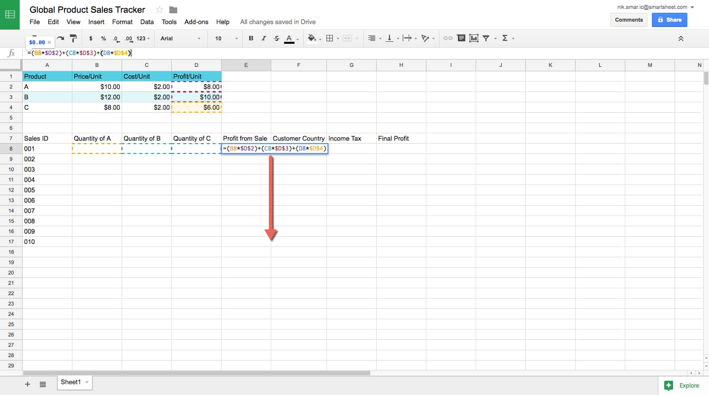
This is one of the more complicated formulas in this article. To calculate the base profit from each sale, we have to multiply each product quantity by that product’s profit margin per unit, and add them all together. Click cell 7E and insert this initial formula: “=(B8*D2)+(C8*D3)+(D8*D4).” We include the parenthesis to maintain the order of operation in the formula. However, there’s a problem.
If you drag that formula down to duplicate it for each sale, it will change the relative location of both the reference cell and its multiplier. For example, dragging it down one cell would result in the formula “=(B9*D3)+(C9*D4)+(D9*D5),” which would mean we’re not taking the same profit margin cells and multiplying them by new quantity levels. To fix this problem, you add “$” to the front of each part of the cell coordinate you want to remain constant. The final result will look like this: “=(B8*$D$2)+(C8*$D$3)+(D8*$D$4).”
Now, when you drag the lower right corner of the cell down through all 10 orders, they will all reference the correct profit margin cells in the reference table. Don’t forget to highlight E8 through E18 and click the $ button on the toolbar. This will place everything into “$0.00” form.
Step 6: Calculate a Final Profit and Column Totals
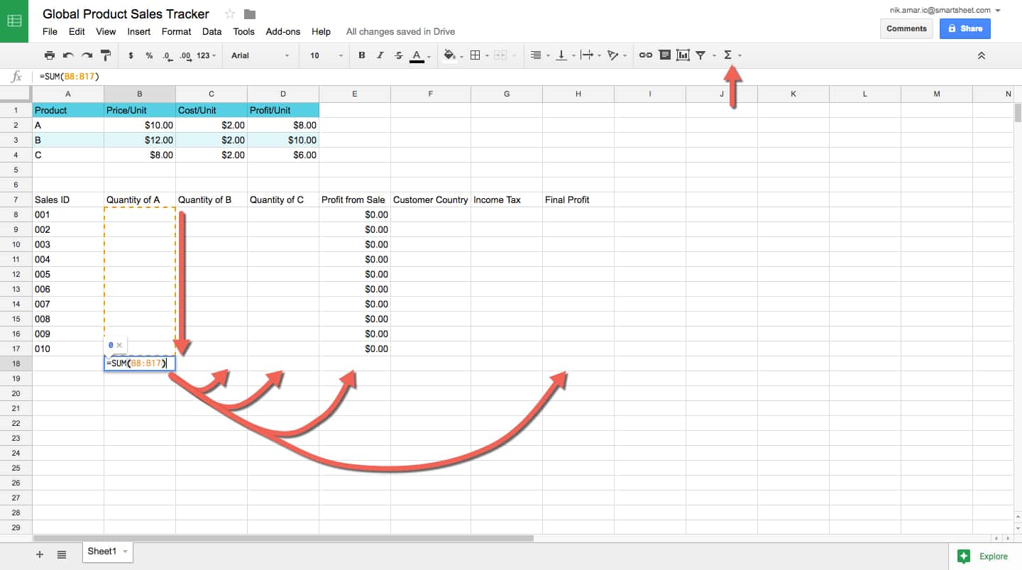
The Final Profit column needs to reflect profit after the customer’s country’s trade taxes. For starters, type “=E8*(1-G8)”. The reason for this is that the Income Tax column will be represented as percentages, where 1 = 100%. Therefore, to subtract the tax rate from the profit, the profit needs to be multiplied by the percentage left over, not the percentage taken out.
Format the Income Tax column by highlighting the cells and clicking the % button on the toolbar. Add the currency format to the Final Profit column by highlighting it’s cells and clicking the $ format button.
Now, use the basic AutoSum formula to place totals counts for each of the quantity columns, for the Profit from Sale column, and the Final Profit column. Highlight B8 through B17, then click the Formula button on the toolbar, and click SUM. The total sum will appear in B18. Now drag this cell’s formula to C18 and D18, then copy and paste it into H18.
Step 7: Add Styling
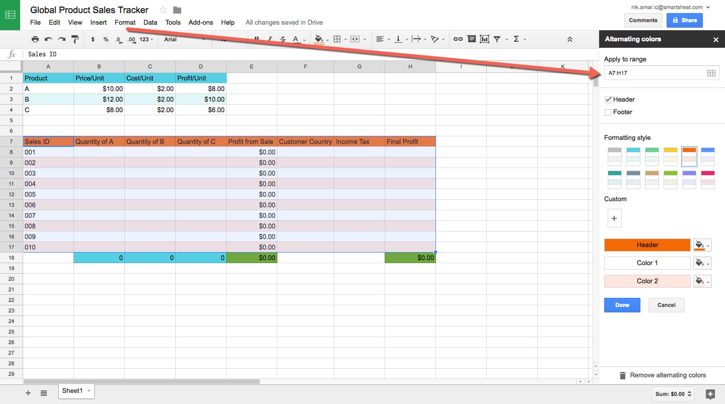
Add styling to your table to help make it more readable. Click and highlight all the cells in the table (excluding the totals). Then click the Format menu and click Alternating Colors in the drop-down menu. Then click a Formatting Style from the sidebar to apply a style to your table. Click the blue Done button.
Next, click and highlight the cells containing totals totals, and click the Fill Color icon on the toolbar and choose a color. Quantity totals might have the same color as the product reference table above. Totals relating to money might be green. Adding color elements to help with quick visual reference is a plus.
Step 8: Enter Data
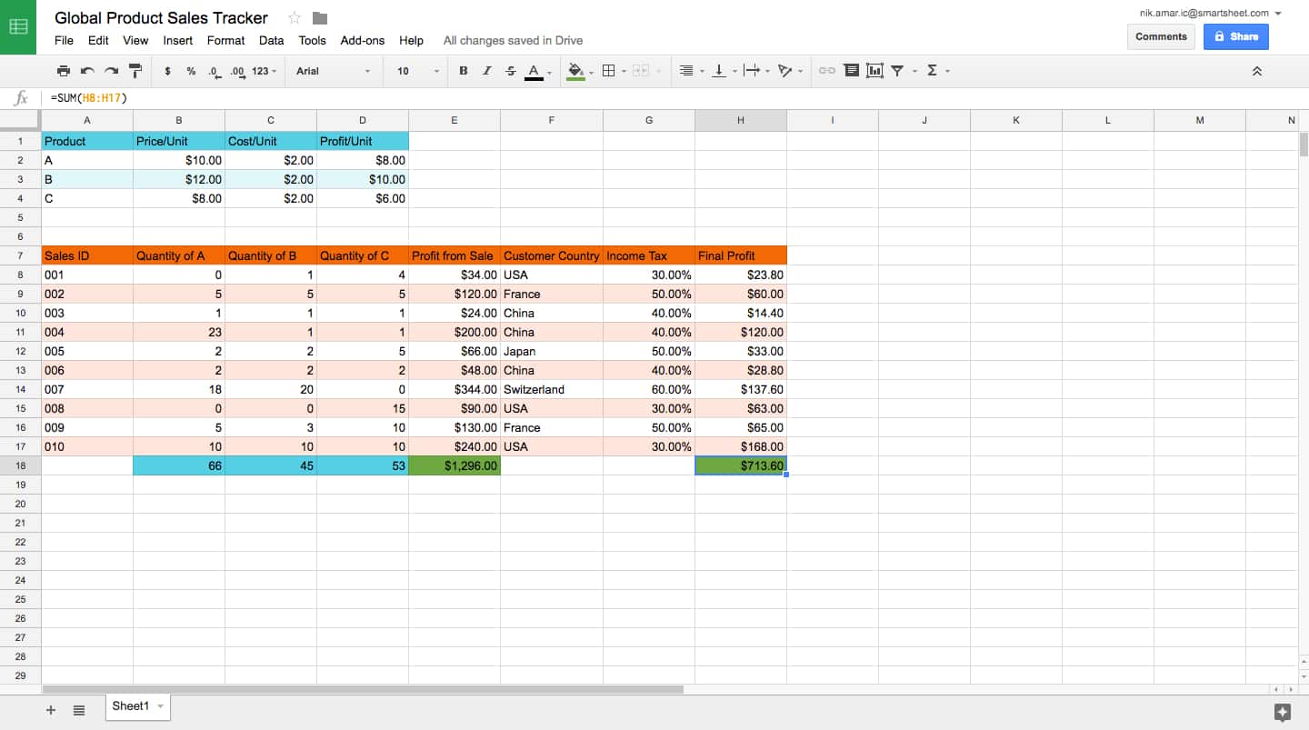
Now enter data for all your table’s quantities sold for every product in every sale, and the buyer’s country. Feel free to use the data in the screenshot above. You’ll notice all the calculations are done automatically.
Step 9: Sort by Country
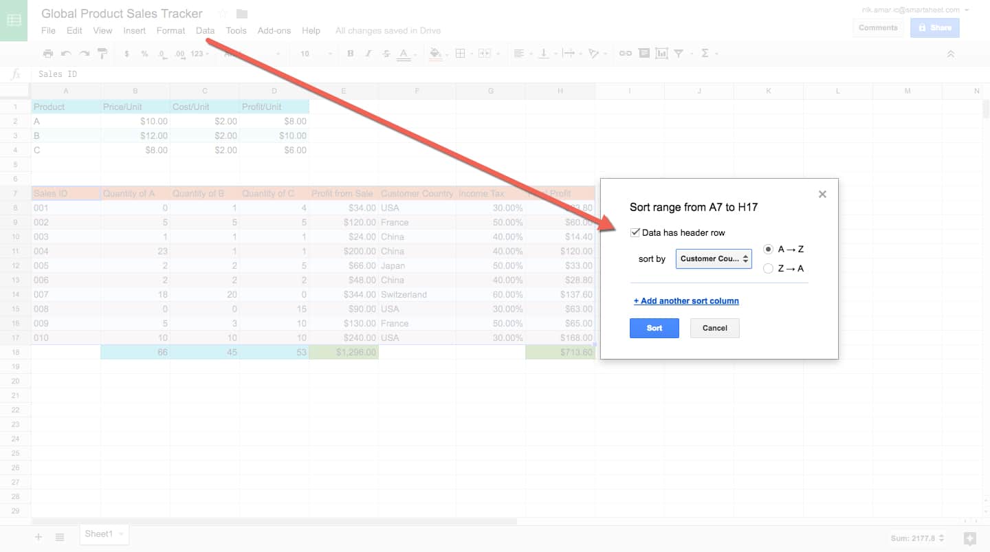
Let’s learn about sorting. To create a table for map data, we have to have totals by country. It’ll be easier to gather this data if we sort it by that criteria. You want to be sure when sorting that you don’t cause any rows to become disassembled — data has to remain together to be useful.
Select A7 through H17 (this is the entire table except the totals). Now open the Data menu, click Sort range, and then tick the Data has header row box. (It won’t rearrange the headers, just everything underneath them.) Then choose the column Customer Country from the sort by menu, going from A to Z. Now your data is arranged by country.
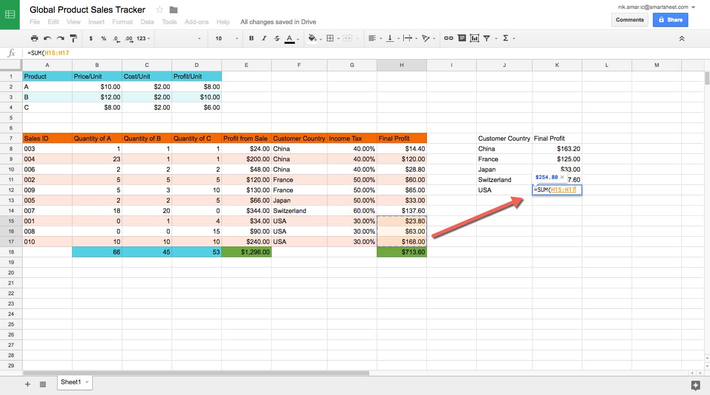
Now use the same steps described above to create a table with just the Customer Country and the Final Profit as headers. Each country only gets one cell, and the Final Profit is the added profit from that country using the formula “=SUM(start cell : end cell).” For the USA, click on cell K12 and type the formula “=SUM(H15:H217).” You’ll need to add each formula manually. You can add styling to it too, if you like.
Step 10: Analyze Data with Explore
Now that you have your data represented to answer all your questions, it’s time to start analyzing them. It’s important to remember that on a real sales sheet, you would likely have 100s of 1000s of sales, not 10, so computer-assisted analysis would be truly beneficial.
Click the Explore icon in the bottom right corner of your screen to open the Explore sidebar. As you can see from the gif, there are countless ways to analyze the data by selecting one table or another, and exploring the auto-created charts and graphs available. You can also highlight all the cells in a table and click Chart. Now you have a working sales tracker with helpful data analysis ready to go.
Here’s a complete list of keyboard shortcuts in Google Sheets.
How to Make a Spreadsheet in Smartsheet: Step-by-Step Guide
This section will cover all the basics you need to know about working with Smartsheet, a spreadsheet-inspired work and process automation platform that you can use to create powerful, collaborative spreadsheets. It’s a cloud-based application, so you never have to download anything, and it can be updated from any computer or smartphone and stays synced across devices. It is available on any platform with a web browser and you can share spreadsheets with anyone.
Unique Features of Smartsheet
Smartsheet has many, though not all, of the functions that Excel has in a real-time collaborative environment. What makes Smartsheet unique is that spreadsheets, known as Grid View, are only the underlying basis for the app’s capabilities. With Smartsheet you can assign unique properties to each column that affect its behavior in different view-types. For example, if you have a Date column, you can view your data in Calendar View, where each row becomes an item on a calendar. If you give each row a Start Date and End Date column, you can use Gantt View to see where timelines overlap from item to item. If you give your rows a Dropdown List column, you can use Card View to see items as cards that you can drag and drop from one section to another, to denote category or status.
One other major unique feature of Smartsheet is that not everyone needs to purchase the app in order to access it. One paid user can invite internal and external collaborators to a sheet, who can all collaborate on the sheet in real time.
How to Create a Project Tracker Spreadsheet in Smartsheet
You can practice making your own project tracker spreadsheet from scratch in Smartsheet. This guide will cover basics and many of the app’s unique features to quickly produce a powerful, collaborative spreadsheet.
Step 1: Create a New Sheet and Name It
On the homepage of Smartsheet, Click Create and choose Grid to get started.
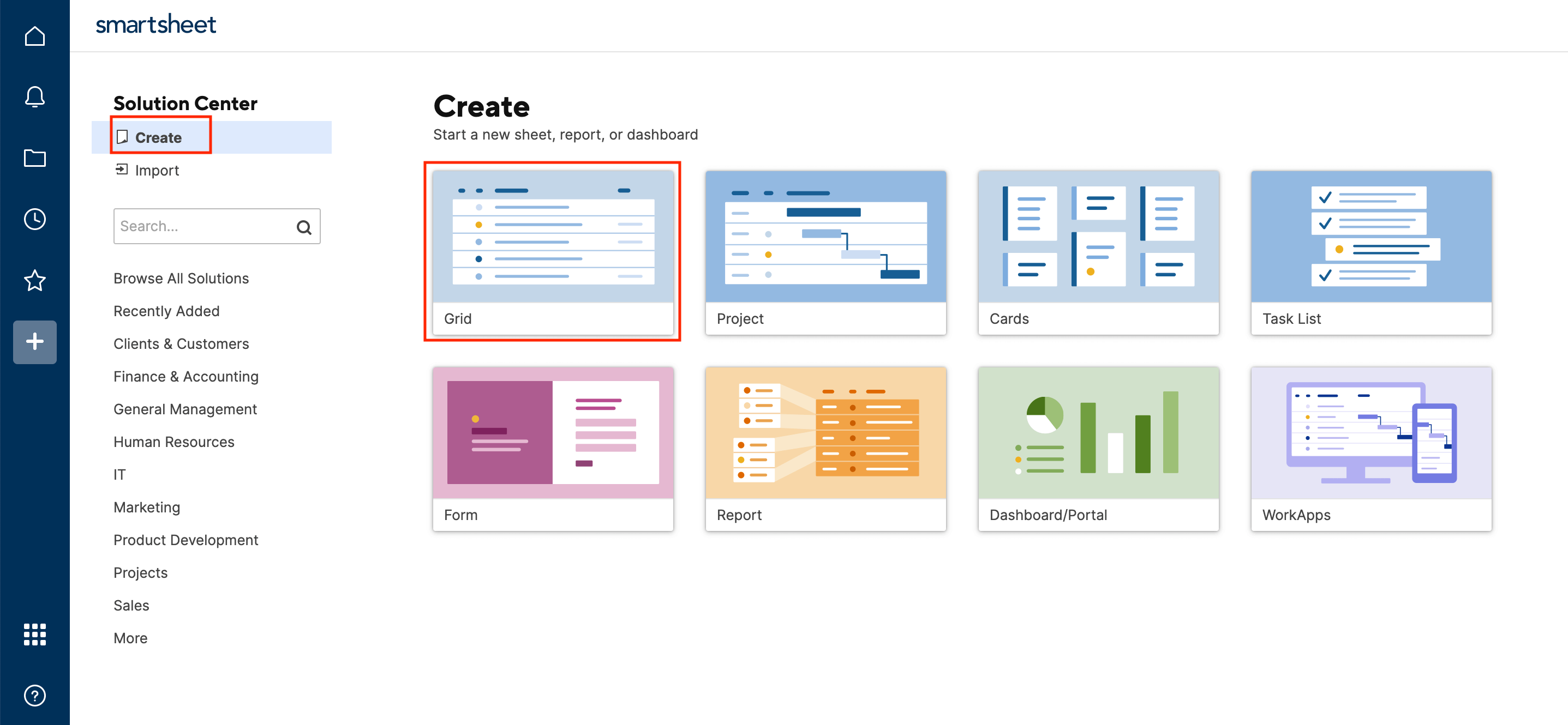
In the popup window, name your sheet “New Project Sheet.”

Step 2: Name Your Primary Column and Enter Data
Start by changing the name of your Primary Column to “Task Name.” Click the cell with the words Primary Column to rename it in the pop-up window that appears on the screen. Click the blue OK button.
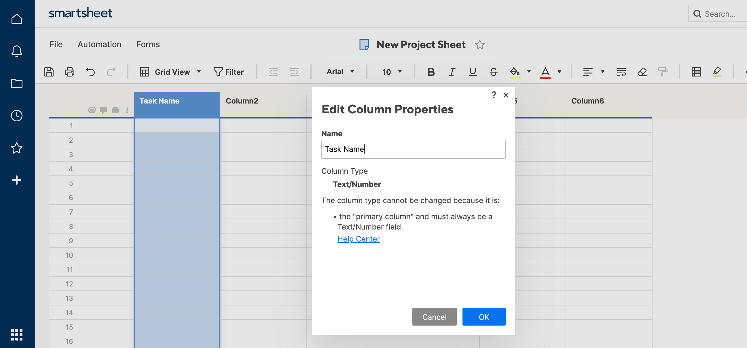
Enter a couple tasks in the column related to whatever you like.

Step 3: Create a Contact List Column
Now change the name of Column2 to “Assigned To.” Click the cell with the words Column2 to rename it in the pop-up window that appears on the screen. Then, click the column property Contact List. Click OK.
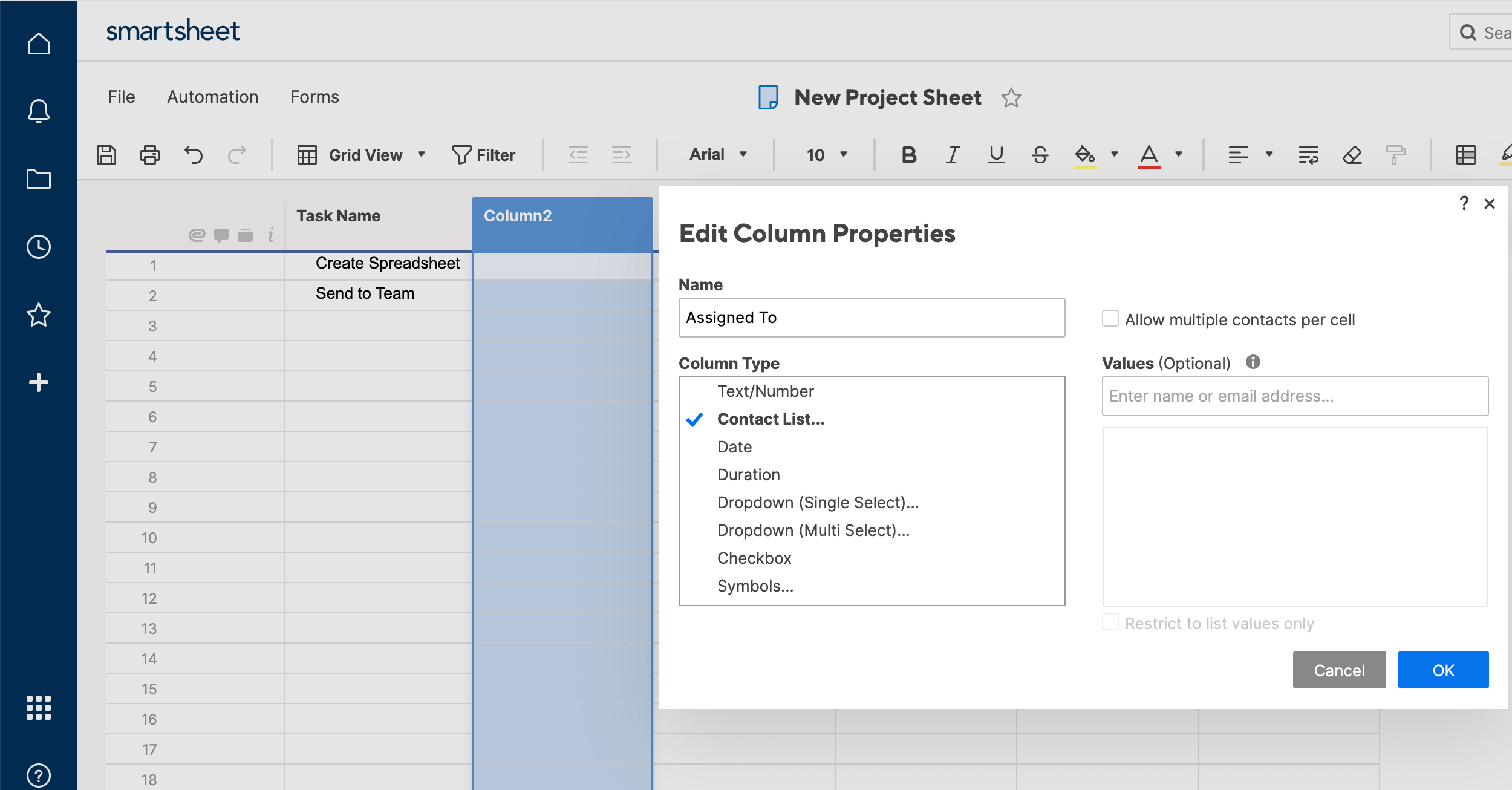
Now you can start typing here in each row of this column, and Smartsheet will autofill names from your contacts to assign tasks to them.
Step 4: Create Start and End Date Columns
Click on the Column3 and Column4 cell to rename them “Start” and “Due,” respectively. Change both their column properties to Date. This will allow you to use both Calendar View and Gantt View, which are useful views when managing large spreadsheets or project data.
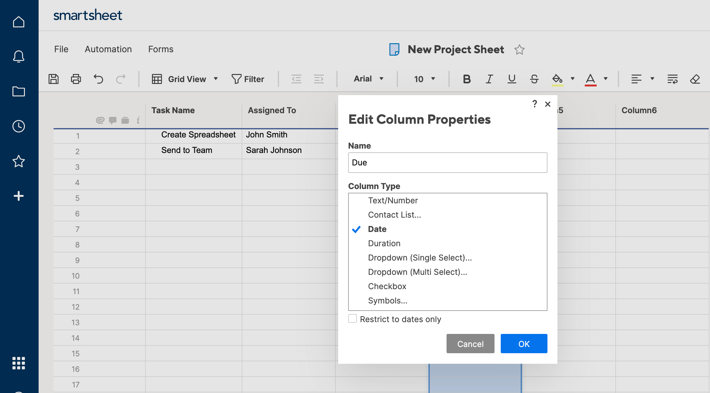
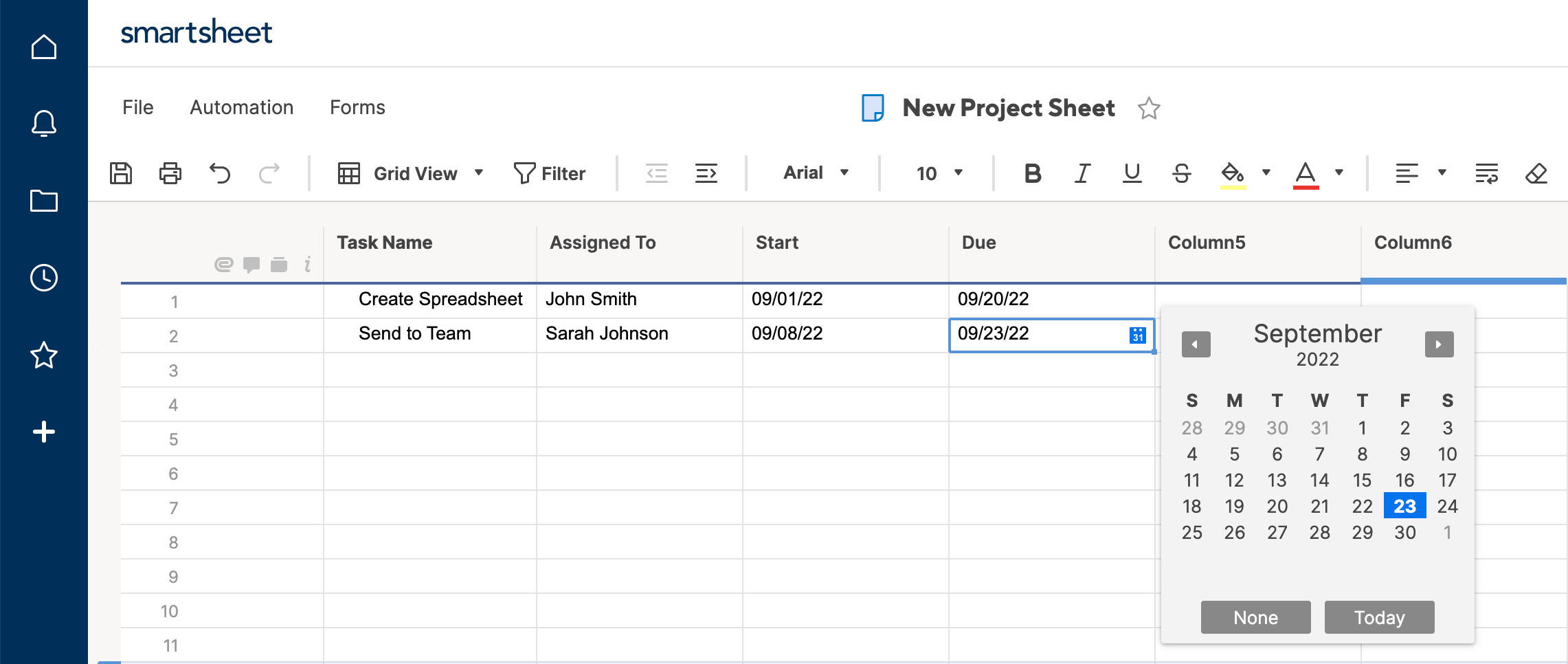
Step 5: Create a Drop Down List Column
Change the name of Column5 to “Stage,” and give it the Dropdown List property. Dropdown List lets you choose a few different options for collaborators to select. It also allows you to use Card View to organize information from grid view by task status (or another criteria of your choosing). You can select either Single Select or Multi-Select options, meaning users can either select only one option, or multiple options, respectively.
For this sheet, select Single Select, and make your status options “Not Started,” “In Progress,” “In Review,” and “Complete.”
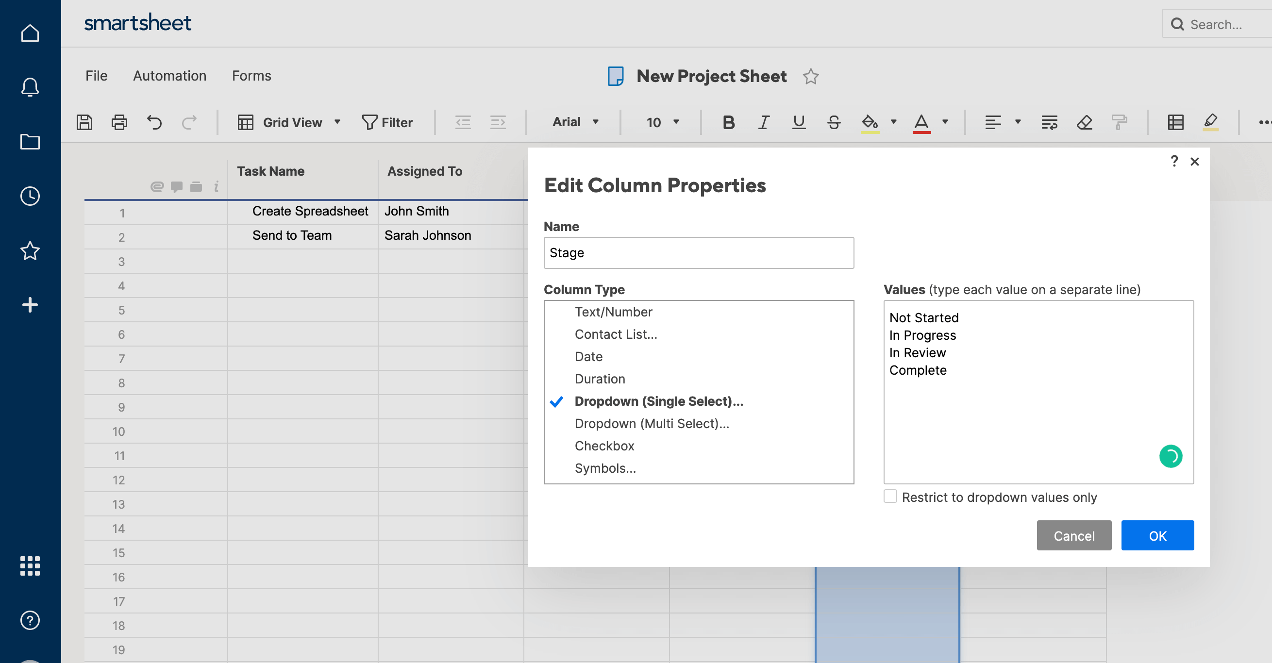
Step 6: Create a Symbols Column
Change the name of Column6 to “Status,” and give it the Symbols column property. This is like a dropdown list, but uses different symbols to represent information about your row, at a glance. In this case, use the RYG balls, which are colored either Red, Yellow, or Green. Red means “late,” yellow means “almost late,” and green means “on time.”
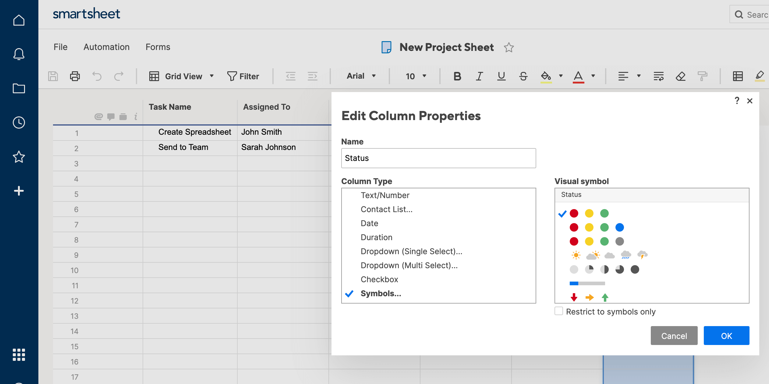
Step 7: Look at Gantt View
Now you have a working project management sheet that’s easy to collaborate on and view multiple ways. Once you enter dates for each task in the Start and Due columns, select Gantt View from the top navigation bar, and to see how your tasks overlap based on start and end dates.
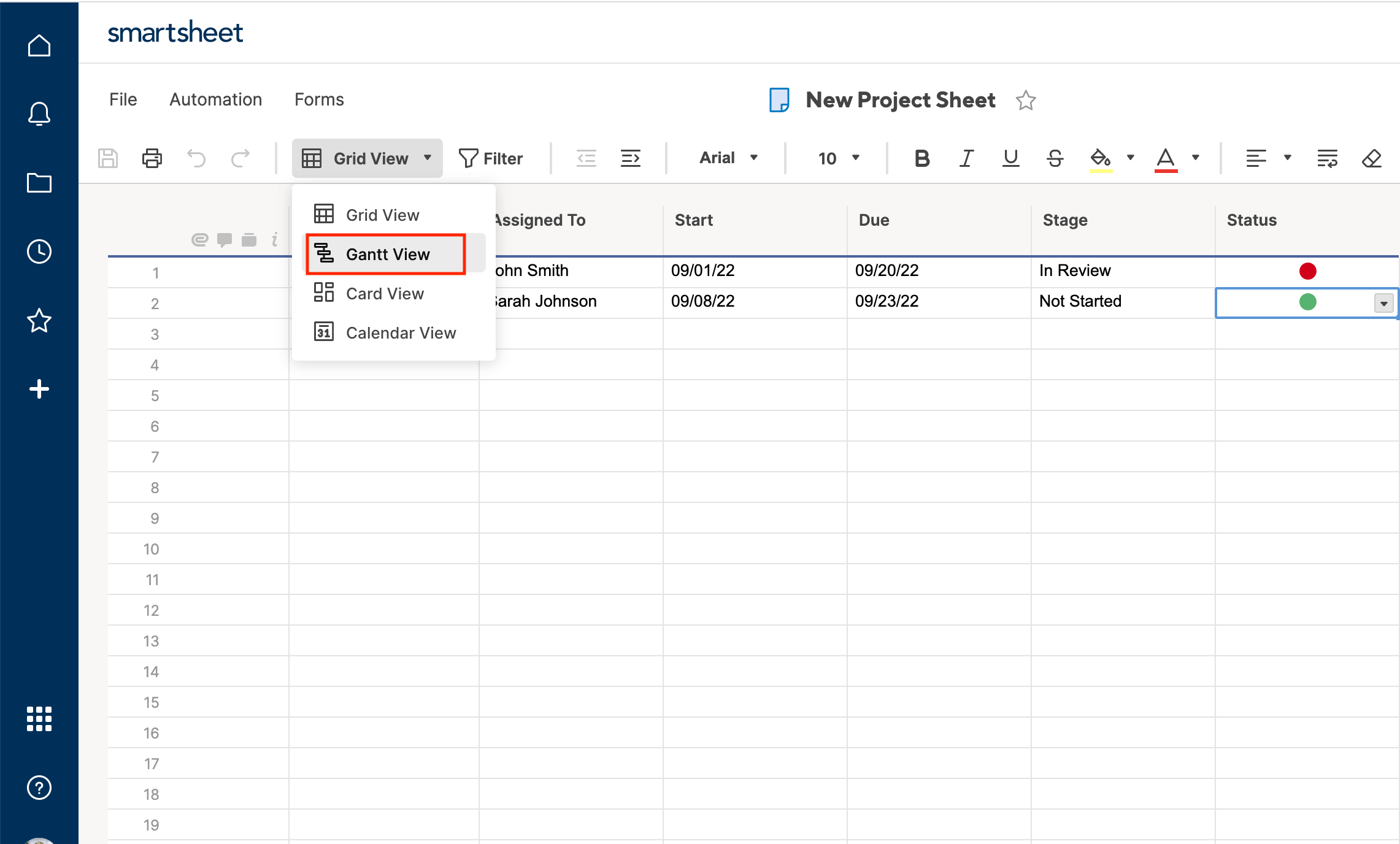
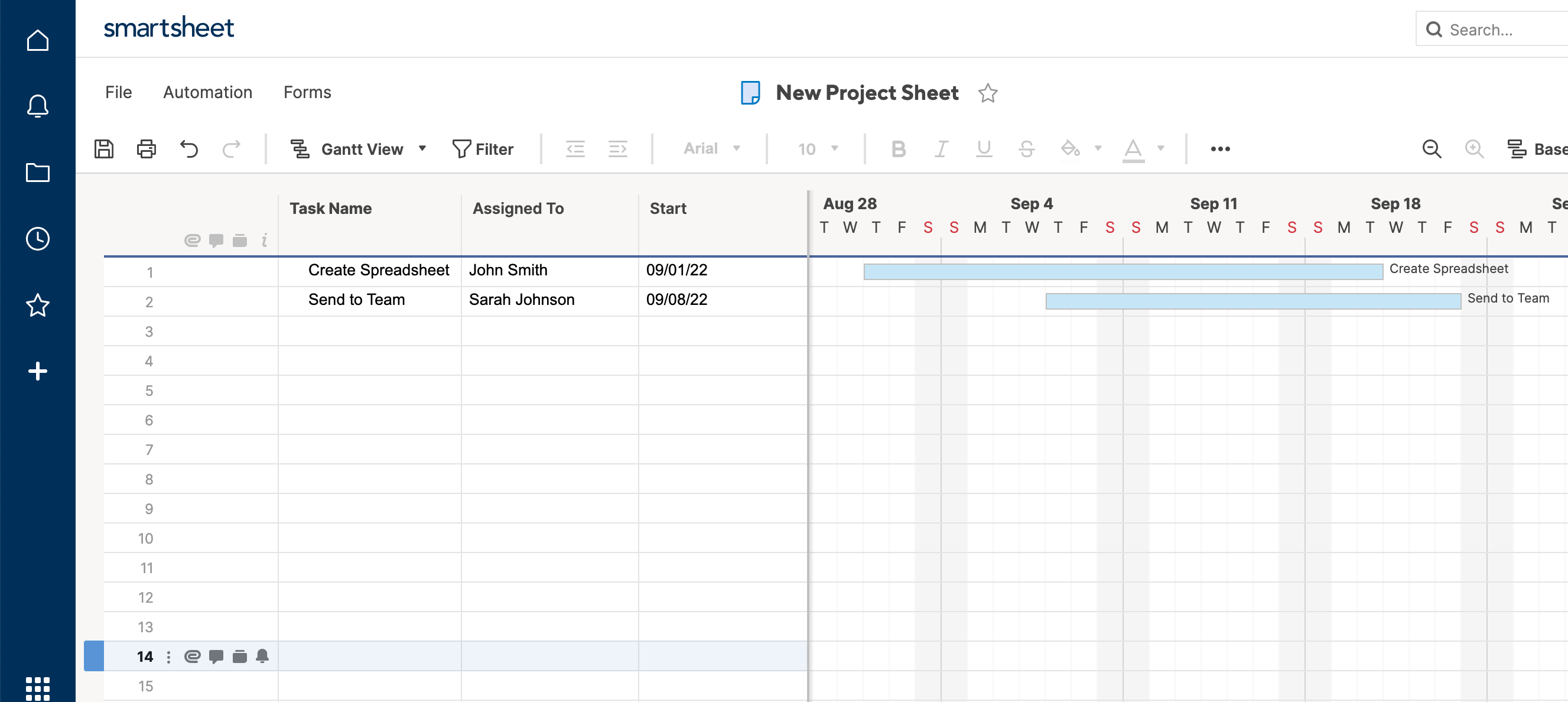
Step 8: Look at Card View
With Card View, you can view all of your task rows by Stage, because Stage is a criteria in your Dropdown List. This is a quick visual way to see how many tasks are outstanding, and where work is getting stuck. When you change from Not Started to In Progress, you can just click the card, and drag it over to the next column. When you go back to Grid View, the status change will be reflected there, too.
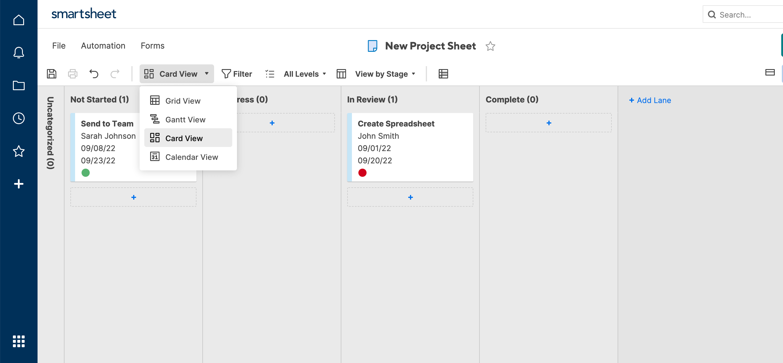
Step 9: Look at Calendar View
When you go to Calendar View with multiple date columns, it asks how you want to handle them. Click Display Date Ranges Using and set Start as the start date, and Due as the end date. Now you can view the stretch of time you’re supposed to work on each task.
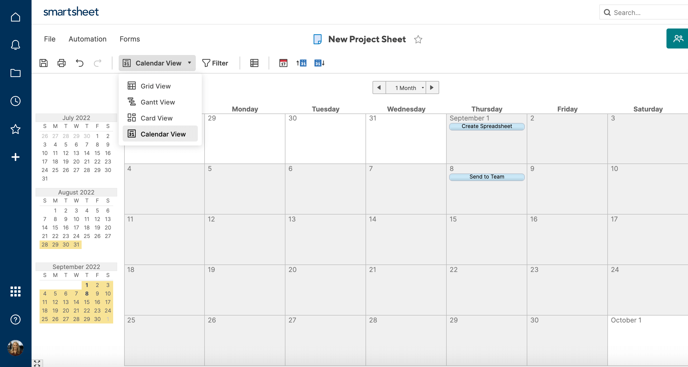
Just like that, you have a basic, flexible project management sheet ready to go. There’s a lot more you can do with Smartsheet, including adding traditional formulas, but this example demonstrates many of its unique features.
Spreadsheet Use Cases and Templates
Now you know how to build a spreadsheet from scratch in Excel, Word, Google Sheets, and Smartsheet. However, all of these programs also have pre-built, use case-specific templates that will save you time. Here are a few popular templates for each of these programs, so you can start organizing and calculating anything you want.
Budget Templates
- Monthly Budget for Google Sheets
- Expense Report for Google Sheets
- Balance Sheet for Smartsheet
Scheduling Templates
- Calendar Template in Google Sheets
- Weekly Schedule in Microsoft Excel
- To Do List in Microsoft Excel
Work and Employee Management Templates
- Employee Timesheet in Microsoft Excel
- Work Schedule Template in Smartsheet
- Project Management Template in Smartsheet
These are just a sampling of the many personal, industry-specific, or project-specific templates that these programs have to offer.
Create a More Powerful, Collaborative Spreadsheet in Smartsheet
Empower your people to go above and beyond with a flexible platform designed to match the needs of your team — and adapt as those needs change.
The Smartsheet platform makes it easy to plan, capture, manage, and report on work from anywhere, helping your team be more effective and get more done. Report on key metrics and get real-time visibility into work as it happens with roll-up reports, dashboards, and automated workflows built to keep your team connected and informed.
When teams have clarity into the work getting done, there’s no telling how much more they can accomplish in the same amount of time. Try Smartsheet for free, today.
Different applications generate data in different forms.
A SaaS application might generate a report in the form of a PDF, while another application might generate data in the form of a TXT or CSV file.
The challenge lies in consolidating the data into a single application that can work with all the data to produce the required results.
Microsoft Excel is one application that is frequently used for this, owing to its versatility in importing data from files with a wide variety of extensions.
For example, if you have a list of items saved in a Text file (or in Notepad), Excel allows you to import this list so that you can process it further.
In this tutorial we will show you two ways to convert a text file to Excel:
- By using the Text Import Wizard
- By opening the file directly in Excel
What is a Text File?
A Text file is one that contains text with no special formatting (as in bold, italic, images, etc.).
These files are identified with the ‘.txt’ extension and can be opened in any text editor, like Notepad or word processor, like Microsoft Word.
But in many cases, you can have data in a text file that you need to open in Excel and analyze there.
Thankfully, you can easily open text files in Microsoft Excel and then further work on it.
Let’s see how to do that!
Let us look at two ways in which we can convert a Text file (.txt) to Excel.
Method 1: Using the Text Import Wizard to Convert a Text File to Excel
If you have a spreadsheet open in Excel and want to import the contents of a Text file at a specific area of your spreadsheet, the Text Import Wizard might be the best way to go.
This wizard scans your text file and ensures that the data in the file is imported the way you want.
To use the Text Import Wizard, select the Data tab, followed by ‘From Text’ (which you will find under the ‘Get External Data’ group.
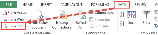
After this, select the text file that you want to import.
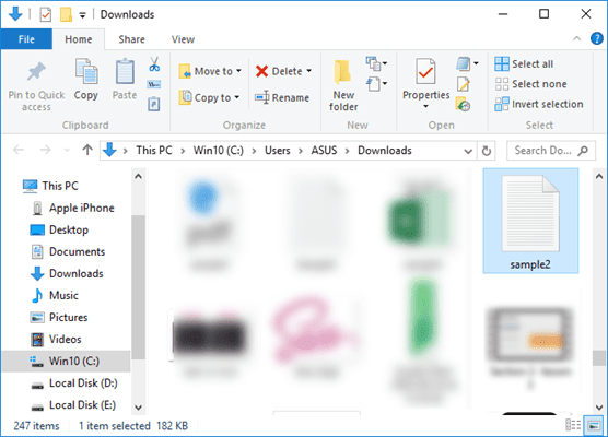
Your Text Import Wizard should now open automatically.
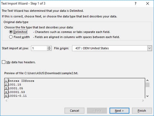
The Text Import Wizard guides you in providing the best settings to import your text file data through 3 steps:
Step 1 of 3
In this step you can provide the settings for the following:
- Original Data Type: Here you can choose how you want your data to be separated into columns. You have two options:
- Delimited: Select this if your text file data is separated by tabs, colons, semicolons or other characters.
- Fixed width: Select this if all items in each column of your data are the same width.
- Start import at row: Type or select the first row of your data from where you want to start importing.
- File origin: Select the character set that your text file uses, for example 437 (for the OEM United States character set). Usually, it’s fine to leave this at the default setting.
- My data has headers: Keep this field checked if your Text file’s dataset contains headers.

Step 2 of 3
If you had selected the ‘Delimited’ radio button in Step 1, then this step lets you specify the delimiters that your data contains (for example tabs, commas, semicolons, etc.) You can also specify if you want consecutive delimiters to be counted as one.
Moreover, if your text values are enclosed in a special set of characters (for example in single or double quotes), then you can specify the character in this step.
These characters are known as ‘Text qualifiers’ and help specify if you want a set of values to be imported as one.
For example, “Scott, Steve” is imported as a single value, even though the words are separated by a comma delimiter.

At the bottom of the screen, you can see a preview of how your data will get affected in the spreadsheet after conversion.
If you had selected the ‘Fixed Width’ radio button in Step 1, on the other hand, then Step 2 lets you specify widths for each column.
You can introduce a new column break in the preview window by simply clicking at the appropriate point on the scale.
A line with an arrow should appear to represent the column break.
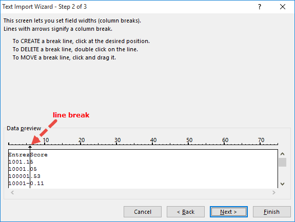
Place line breaks wherever you need to in the preview window.
If you want to move a line break, simply drag it across. If you want to remove a line, simply double-click on it.
Step 3 of 3
This lets you specify the data format for each column.
You can specify if you want a column to remain in the default format set by the Text Import Wizard or if you want to set the format to be General, Text, or Date.
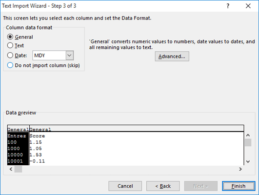
Simply select a column from the preview window and select the format you want.
If you want to remove a selected column, select the last radio button option (which says ‘Do not import column‘).
The Advanced button in this step opens the Advanced Text Import Settings dialog box.
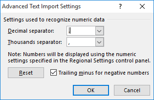
This dialog box lets you specify advanced formatting options.
For example, you can use the Advanced Text Import Settings to specify what decimal or thousands separators have been used in the text file, so that they can be made to match your computer’s regional settings.
Once you’re done providing all the settings for your imported text data, click on the Finish button.
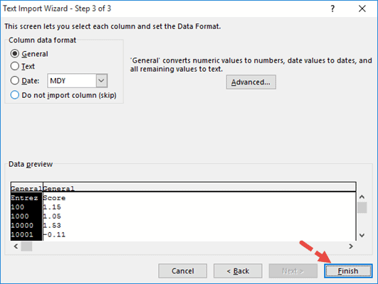
This will open the Import Data dialog box.
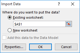
In this box, you can select where you want your text file’s data imported.
If you want to import it into the existing worksheet, you can select or type in a reference to the cell where you want Excel to start displaying the imported data.
If you want to open it in a new worksheet, however, then select the radio button next to ‘New Worksheet’.
Click OK.
Your text file should now get imported to your selected location in Excel, with the format settings that you had specified in the Text Import Wizard.

Also read: How to Open XML Files in Excel?
Method 2: Opening a Text File Directly in Excel
You can also choose to simply open the text file directly in Excel.
While opening, Excel recognizes a text file and automatically converts it into a format that can be displayed in a spreadsheet.
All you need to do is click on the File tab, select Open and then browse and select the text file that you want to open.
One issue that you are likely to face when trying to open a text file directly in Excel is trying to locate the file in the folder.
This is because Excel’s ‘Open File’ dialog box, by default, filters, and displays only Excel files like those with extensions ‘.xls’, ‘.xlsx’, etc.
It also displays CSV files, if your computer is set up to use Excel as the default application to open CSV files.
So if you don’t see your required text file in the folder when trying to open it in Excel, simply select ‘All Files’ from the ‘File Types’ drop-down, as shown below:
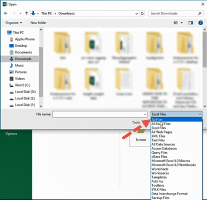
This will display the Text Import Wizard from where you can set up how you want your Text file’s data to be displayed in Excel (as shown in method 1).

You should now see your text file converted and displayed in Excel.
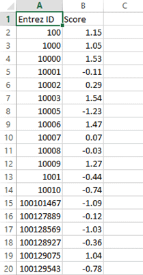
Once the file opens, if you still find some of the columns (or individual cells) not converted to your required format, you can convert them manually.
While this method to open the Text file directly in Excel works well, the benefit of using the first method (using Text Import Wizard) allows you to make some adjustments even before getting the data in Excel.
In this tutorial, we showed you two ways to convert and open a Text file in Excel.
A third method could be by using online tools like Online2pdf, but we did not dwell too much on this because Excel’s Text Import Wizard provides much more flexibility, allowing you to adjust your data, and format them exactly how you want them.
We hope this tutorial was helpful for you.
Other Excel tutorials you may also like:
- How to Convert a CSV File to Excel?
- How to Open VCF File in Excel?
- How to Open Excel File [xls, xlsx] Online (for FREE)
- Why does Excel Open on Startup (and How to Stop it)
- How to Make Excel File Read Only
- How to Insert an Excel file into MS Word
- How to Save Selection in Excel as PDF (3 Easy Methods)
- How to Merge Two Excel Files?
- How to Convert PDF to Excel without Software?
- How to Open DAT Files in Excel?