
The TEXT function lets you change the way a number appears by applying formatting to it with format codes. It’s useful in situations where you want to display numbers in a more readable format, or you want to combine numbers with text or symbols.
Note: The TEXT function will convert numbers to text, which may make it difficult to reference in later calculations. It’s best to keep your original value in one cell, then use the TEXT function in another cell. Then, if you need to build other formulas, always reference the original value and not the TEXT function result.
Syntax
TEXT(value, format_text)
The TEXT function syntax has the following arguments:
|
Argument Name |
Description |
|
value |
A numeric value that you want to be converted into text. |
|
format_text |
A text string that defines the formatting that you want to be applied to the supplied value. |
Overview
In its simplest form, the TEXT function says:
-
=TEXT(Value you want to format, «Format code you want to apply»)
Here are some popular examples, which you can copy directly into Excel to experiment with on your own. Notice the format codes within quotation marks.
|
Formula |
Description |
|
=TEXT(1234.567,«$#,##0.00») |
Currency with a thousands separator and 2 decimals, like $1,234.57. Note that Excel rounds the value to 2 decimal places. |
|
=TEXT(TODAY(),«MM/DD/YY») |
Today’s date in MM/DD/YY format, like 03/14/12 |
|
=TEXT(TODAY(),«DDDD») |
Today’s day of the week, like Monday |
|
=TEXT(NOW(),«H:MM AM/PM») |
Current time, like 1:29 PM |
|
=TEXT(0.285,«0.0%») |
Percentage, like 28.5% |
|
=TEXT(4.34 ,«# ?/?») |
Fraction, like 4 1/3 |
|
=TRIM(TEXT(0.34,«# ?/?»)) |
Fraction, like 1/3. Note this uses the TRIM function to remove the leading space with a decimal value. |
|
=TEXT(12200000,«0.00E+00») |
Scientific notation, like 1.22E+07 |
|
=TEXT(1234567898,«[<=9999999]###-####;(###) ###-####») |
Special (Phone number), like (123) 456-7898 |
|
=TEXT(1234,«0000000») |
Add leading zeros (0), like 0001234 |
|
=TEXT(123456,«##0° 00′ 00»») |
Custom — Latitude/Longitude |
Note: Although you can use the TEXT function to change formatting, it’s not the only way. You can change the format without a formula by pressing CTRL+1 (or  +1 on the Mac), then pick the format you want from the Format Cells > Number dialog.
Download our examples
You can download an example workbook with all of the TEXT function examples you’ll find in this article, plus some extras. You can follow along, or create your own TEXT function format codes.
Download Excel TEXT function examples
Other format codes that are available
You can use the Format Cells dialog to find the other available format codes:
-
Press Ctrl+1 (
 +1 on the Mac) to bring up the Format Cells dialog.
 -
Select the format you want from the Number tab.
-
Select the Custom option,
-
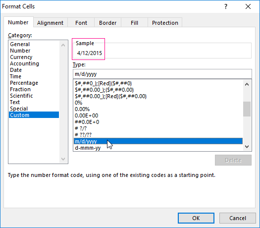
The format code you want is now shown in the Type box. In this case, select everything from the Type box except the semicolon (;) and @ symbol. In the example below, we selected and copied just mm/dd/yy.
-
Press Ctrl+C to copy the format code, then press Cancel to dismiss the Format Cells dialog.
-
Now, all you need to do is press Ctrl+V to paste the format code into your TEXT formula, like: =TEXT(B2,»mm/dd/yy«). Make sure that you paste the format code within quotes («format code»), otherwise Excel will throw an error message.

Format codes by category
Following are some examples of how you can apply different number formats to your values by using the Format Cells dialog, then use the Custom option to copy those format codes to your TEXT function.
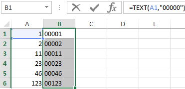
Why does Excel delete my leading 0’s?
Excel is trained to look for numbers being entered in cells, not numbers that look like text, like part numbers or SKU’s. To retain leading zeros, format the input range as Text before you paste or enter values. Select the column, or range where you’ll be putting the values, then use CTRL+1 to bring up the Format > Cells dialog and on the Number tab select Text. Now Excel will keep your leading 0’s.
If you’ve already entered data and Excel has removed your leading 0’s, you can use the TEXT function to add them back. You can reference the top cell with the values and use =TEXT(value,»00000″), where the number of 0’s in the formula represents the total number of characters you want, then copy and paste to the rest of your range.
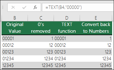
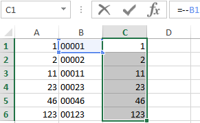
If for some reason you need to convert text values back to numbers you can multiply by 1, like =D4*1, or use the double-unary operator (—), like =—D4.
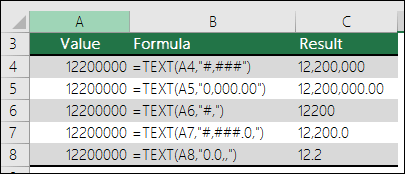
Excel separates thousands by commas if the format contains a comma (,) that is enclosed by number signs (#) or by zeros. For example, if the format string is «#,###», Excel displays the number 12200000 as 12,200,000.
A comma that follows a digit placeholder scales the number by 1,000. For example, if the format string is «#,###.0,», Excel displays the number 12200000 as 12,200.0.
Notes:
-
The thousands separator is dependent on your regional settings. In the US it’s a comma, but in other locales it might be a period (.).
-
The thousands separator is available for the number, currency and accounting formats.
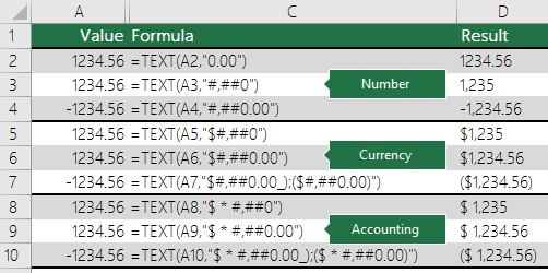
Following are examples of standard number (thousands separator and decimals only), currency and accounting formats. Currency format allows you to insert the currency symbol of your choice and aligns it next to your value, while accounting format will align the currency symbol to the left of the cell and the value to the right. Note the difference between the currency and accounting format codes below, where accounting uses an asterisk (*) to create separation between the symbol and the value.
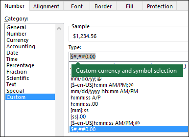
To find the format code for a currency symbol, first press Ctrl+1 (or +1 on the Mac), select the format you want, then choose a symbol from the Symbol drop-down:
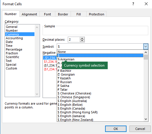
Then click Custom on the left from the Category section, and copy the format code, including the currency symbol.
Note: The TEXT function does not support color formatting, so if you copy a number format code from the Format Cells dialog that includes a color, like this: $#,##0.00_);[Red]($#,##0.00), the TEXT function will accept the format code, but it won’t display the color.
You can alter the way a date displays by using a mix of «M» for month, «D» for days, and «Y» for years.
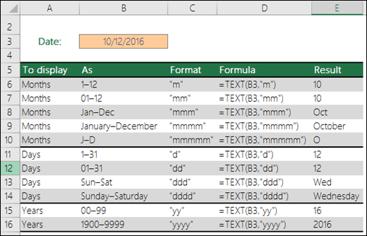
Format codes in the TEXT function aren’t case sensitive, so you can use either «M» or «m», «D» or «d», «Y» or «y».
You can alter the way time displays by using a mix of «H» for hours, «M» for minutes, or «S» for seconds, and «AM/PM» for a 12-hour clock.
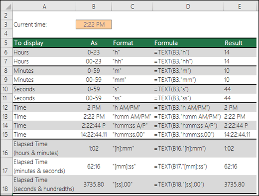
If you leave out the «AM/PM» or «A/P», then time will display based on a 24-hour clock.
Format codes in the TEXT function aren’t case sensitive, so you can use either «H» or «h», «M» or «m», «S» or «s», «AM/PM» or «am/pm».
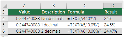
You can alter the way decimal values display with percentage (%) formats.
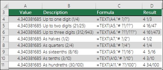
You can alter the way decimal values display with fraction (?/?) formats.
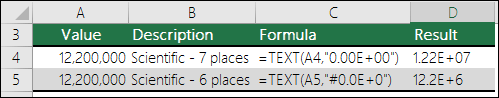
Scientific notation is a way of displaying numbers in terms of a decimal between 1 and 10, multiplied by a power of 10. It is often used to shorten the way that large numbers display.
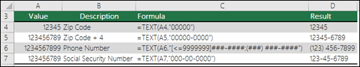
Excel provides 4 special formats:
-
Zip Code — «00000»
-
Zip Code + 4 — «00000-0000»
-
Phone Number — «[<=9999999]###-####;(###) ###-####»
-
Social Security Number — «000-00-0000»
Special formats will be different depending on locale, but if there aren’t any special formats for your locale, or if these don’t meet your needs then you can create your own through the Format Cells > Custom dialog.
Common scenario
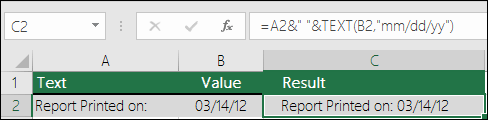
The TEXT function is rarely used by itself, and is most often used in conjunction with something else. Let’s say you want to combine text and a number value, like “Report Printed on: 03/14/12”, or “Weekly Revenue: $66,348.72”. You could type that into Excel manually, but that defeats the purpose of having Excel do it for you. Unfortunately, when you combine text and formatted numbers, like dates, times, currency, etc., Excel doesn’t know how you want to display them, so it drops the number formatting. This is where the TEXT function is invaluable, because it allows you to force Excel to format the values the way you want by using a format code, like «MM/DD/YY» for date format.
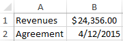
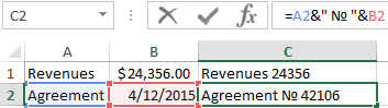
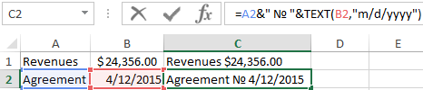
In the following example, you’ll see what happens if you try to join text and a number without using the TEXT function. In this case, we’re using the ampersand (&) to concatenate a text string, a space (» «), and a value with =A2&» «&B2.
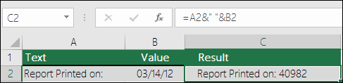
As you can see, Excel removed the formatting from the date in cell B2. In the next example, you’ll see how the TEXT function lets you apply the format you want.
Our updated formula is:
-
Cell C2:=A2&» «&TEXT(B2,»mm/dd/yy») — Date format
Frequently Asked Questions
Yes, you can use the UPPER, LOWER and PROPER functions. For example, =UPPER(«hello») would return «HELLO».
Yes, but it takes a few steps. First, select the cell or cells where you want this to happen and use Ctrl+1 to bring up the Format > Cells dialog, then Alignment > Text control > check the Wrap Text option. Next, adjust your completed TEXT function to include the ASCII function CHAR(10) where you want the line break. You might need to adjust your column width depending on how the final result aligns.
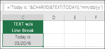
In this case, we used: =»Today is: «&CHAR(10)&TEXT(TODAY(),»mm/dd/yy»)
This is called Scientific Notation, and Excel will automatically convert numbers longer than 12 digits if a cell(s) is formatted as General, and 15 digits if a cell(s) is formatted as a Number. If you need to enter long numeric strings, but don’t want them converted, then format the cells in question as Text before you input or paste your values into Excel.
See Also
Create or delete a custom number format
Convert numbers stored as text to numbers
All Excel functions (by category)
Содержание
- Text functions (reference)
- TEXT function
- Overview
- Download our examples
- Other format codes that are available
- Format codes by category
- Common scenario
- Frequently Asked Questions
Text functions (reference)
To get detailed information about a function, click its name in the first column.
Note: Version markers indicate the version of Excel a function was introduced. These functions aren’t available in earlier versions. For example, a version marker of 2013 indicates that this function is available in Excel 2013 and all later versions.
ARRAYTOTEXT function

Returns an array of text values from any specified range
Changes full-width (double-byte) English letters or katakana within a character string to half-width (single-byte) characters
Converts a number to text, using the ß (baht) currency format
Returns the character specified by the code number
Removes all nonprintable characters from text
Returns a numeric code for the first character in a text string
CONCAT function

Combines the text from multiple ranges and/or strings, but it doesn’t provide the delimiter or IgnoreEmpty arguments.
Joins several text items into one text item
DBCS function

Changes half-width (single-byte) English letters or katakana within a character string to full-width (double-byte) characters
Converts a number to text, using the $ (dollar) currency format
Checks to see if two text values are identical
Finds one text value within another (case-sensitive)
Formats a number as text with a fixed number of decimals
Returns the leftmost characters from a text value
Returns the number of characters in a text string
Converts text to lowercase
Returns a specific number of characters from a text string starting at the position you specify
NUMBERVALUE function
Converts text to number in a locale-independent manner
Extracts the phonetic (furigana) characters from a text string
Capitalizes the first letter in each word of a text value
Replaces characters within text
Repeats text a given number of times
Returns the rightmost characters from a text value
Finds one text value within another (not case-sensitive)
Substitutes new text for old text in a text string
Converts its arguments to text
Formats a number and converts it to text
TEXTAFTER function
Returns text that occurs after given character or string
TEXTBEFORE function
Returns text that occurs before a given character or string
TEXTJOIN function
Combines the text from multiple ranges and/or strings
TEXTSPLIT function
Splits text strings by using column and row delimiters
Removes spaces from text
UNICHAR function
Returns the Unicode character that is references by the given numeric value
UNICODE function
Returns the number (code point) that corresponds to the first character of the text
Converts text to uppercase
Converts a text argument to a number
VALUETOTEXT function
Returns text from any specified value
Important: The calculated results of formulas and some Excel worksheet functions may differ slightly between a Windows PC using x86 or x86-64 architecture and a Windows RT PC using ARM architecture. Learn more about the differences.
Источник
TEXT function
The TEXT function lets you change the way a number appears by applying formatting to it with format codes. It’s useful in situations where you want to display numbers in a more readable format, or you want to combine numbers with text or symbols.
Note: The TEXT function will convert numbers to text, which may make it difficult to reference in later calculations. It’s best to keep your original value in one cell, then use the TEXT function in another cell. Then, if you need to build other formulas, always reference the original value and not the TEXT function result.
The TEXT function syntax has the following arguments:
A numeric value that you want to be converted into text.
A text string that defines the formatting that you want to be applied to the supplied value.
Overview
In its simplest form, the TEXT function says:
=TEXT(Value you want to format, «Format code you want to apply»)
Here are some popular examples, which you can copy directly into Excel to experiment with on your own. Notice the format codes within quotation marks.
Currency with a thousands separator and 2 decimals, like $1,234.57. Note that Excel rounds the value to 2 decimal places.
Today’s date in MM/DD/YY format, like 03/14/12
Today’s day of the week, like Monday
Current time, like 1:29 PM
Percentage, like 28.5%
Fraction, like 4 1/3
Fraction, like 1/3. Note this uses the TRIM function to remove the leading space with a decimal value.
Scientific notation, like 1.22E+07
Add leading zeros (0), like 0001234
Note: Although you can use the TEXT function to change formatting, it’s not the only way. You can change the format without a formula by pressing CTRL+1 (or +1 on the Mac), then pick the format you want from the Format Cells > Number dialog.
Download our examples
You can download an example workbook with all of the TEXT function examples you’ll find in this article, plus some extras. You can follow along, or create your own TEXT function format codes.
Other format codes that are available
You can use the Format Cells dialog to find the other available format codes:
Press Ctrl+1 ( +1 on the Mac) to bring up the Format Cells dialog.
Select the format you want from the Number tab.
Select the Custom option,
The format code you want is now shown in the Type box. In this case, select everything from the Type box except the semicolon (;) and @ symbol. In the example below, we selected and copied just mm/dd/yy.
Press Ctrl+C to copy the format code, then press Cancel to dismiss the Format Cells dialog.
Now, all you need to do is press Ctrl+V to paste the format code into your TEXT formula, like: =TEXT(B2,» mm/dd/yy«). Make sure that you paste the format code within quotes («format code»), otherwise Excel will throw an error message.
Cells > Number > Custom dialog to have Excel create format strings for you.» loading=»lazy»>
Format codes by category
Following are some examples of how you can apply different number formats to your values by using the Format Cells dialog, then use the Custom option to copy those format codes to your TEXT function.
Why does Excel delete my leading 0’s?
Excel is trained to look for numbers being entered in cells, not numbers that look like text, like part numbers or SKU’s. To retain leading zeros, format the input range as Text before you paste or enter values. Select the column, or range where you’ll be putting the values, then use CTRL+1 to bring up the Format > Cells dialog and on the Number tab select Text. Now Excel will keep your leading 0’s.
If you’ve already entered data and Excel has removed your leading 0’s, you can use the TEXT function to add them back. You can reference the top cell with the values and use =TEXT(value,»00000″), where the number of 0’s in the formula represents the total number of characters you want, then copy and paste to the rest of your range.
If for some reason you need to convert text values back to numbers you can multiply by 1, like =D4*1, or use the double-unary operator (—), like =—D4.
Excel separates thousands by commas if the format contains a comma (,) that is enclosed by number signs (#) or by zeros. For example, if the format string is «#,###», Excel displays the number 12200000 as 12,200,000.
A comma that follows a digit placeholder scales the number by 1,000. For example, if the format string is «#,###.0,», Excel displays the number 12200000 as 12,200.0.
The thousands separator is dependent on your regional settings. In the US it’s a comma, but in other locales it might be a period (.).
The thousands separator is available for the number, currency and accounting formats.
Following are examples of standard number (thousands separator and decimals only), currency and accounting formats. Currency format allows you to insert the currency symbol of your choice and aligns it next to your value, while accounting format will align the currency symbol to the left of the cell and the value to the right. Note the difference between the currency and accounting format codes below, where accounting uses an asterisk (*) to create separation between the symbol and the value.
To find the format code for a currency symbol, first press Ctrl+1 (or +1 on the Mac), select the format you want, then choose a symbol from the Symbol drop-down:
Then click Custom on the left from the Category section, and copy the format code, including the currency symbol.
Note: The TEXT function does not support color formatting, so if you copy a number format code from the Format Cells dialog that includes a color, like this: $#,##0.00_); [Red]($#,##0.00), the TEXT function will accept the format code, but it won’t display the color.
You can alter the way a date displays by using a mix of «M» for month, «D» for days, and «Y» for years.
Format codes in the TEXT function aren’t case sensitive, so you can use either «M» or «m», «D» or «d», «Y» or «y».

If you share Excel files and reports with users from different countries, then you might want to give them a report in their language. Excel MVP, Mynda Treacy has a great solution in this Excel Dates Displayed in Different Languages article. It also includes a sample workbook you can download.
You can alter the way time displays by using a mix of «H» for hours, «M» for minutes, or «S» for seconds, and «AM/PM» for a 12-hour clock.
If you leave out the «AM/PM» or «A/P», then time will display based on a 24-hour clock.
Format codes in the TEXT function aren’t case sensitive, so you can use either «H» or «h», «M» or «m», «S» or «s», «AM/PM» or «am/pm».
You can alter the way decimal values display with percentage (%) formats.
You can alter the way decimal values display with fraction (?/?) formats.
Scientific notation is a way of displaying numbers in terms of a decimal between 1 and 10, multiplied by a power of 10. It is often used to shorten the way that large numbers display.
Excel provides 4 special formats:
Zip Code — «00000»
Zip Code + 4 — «00000-0000»
Social Security Number — «000-00-0000»
Special formats will be different depending on locale, but if there aren’t any special formats for your locale, or if these don’t meet your needs then you can create your own through the Format Cells > Custom dialog.
Common scenario
The TEXT function is rarely used by itself, and is most often used in conjunction with something else. Let’s say you want to combine text and a number value, like “Report Printed on: 03/14/12”, or “Weekly Revenue: $66,348.72”. You could type that into Excel manually, but that defeats the purpose of having Excel do it for you. Unfortunately, when you combine text and formatted numbers, like dates, times, currency, etc., Excel doesn’t know how you want to display them, so it drops the number formatting. This is where the TEXT function is invaluable, because it allows you to force Excel to format the values the way you want by using a format code, like «MM/DD/YY» for date format.
In the following example, you’ll see what happens if you try to join text and a number without using the TEXT function. In this case, we’re using the ampersand ( &) to concatenate a text string, a space (» «), and a value with =A2&» «&B2.
As you can see, Excel removed the formatting from the date in cell B2. In the next example, you’ll see how the TEXT function lets you apply the format you want.
Our updated formula is:
Cell C2: =A2&» «&TEXT(B2,»mm/dd/yy») — Date format
Frequently Asked Questions
Unfortunately, you can’t do that with the TEXT function, you need to use Visual Basic for Applications (VBA) code. The following link has a method: How to convert a numeric value into English words in Excel
Yes, you can use the UPPER, LOWER and PROPER functions. For example, =UPPER(«hello») would return «HELLO».
Yes, but it takes a few steps. First, select the cell or cells where you want this to happen and use Ctrl+1 to bring up the Format > Cells dialog, then Alignment > Text control > check the Wrap Text option. Next, adjust your completed TEXT function to include the ASCII function CHAR(10) where you want the line break. You might need to adjust your column width depending on how the final result aligns.
In this case, we used: =»Today is: «&CHAR(10)&TEXT(TODAY(),»mm/dd/yy»)
This is called Scientific Notation, and Excel will automatically convert numbers longer than 12 digits if a cell(s) is formatted as General, and 15 digits if a cell(s) is formatted as a Number. If you need to enter long numeric strings, but don’t want them converted, then format the cells in question as Text before you input or paste your values into Excel.
If you share Excel files and reports with users from different countries, then you might want to give them a report in their language. Excel MVP, Mynda Treacy has a great solution in this Excel Dates Displayed in Different Languages article. It also includes a sample workbook you can download.
Источник
На чтение 23 мин. Просмотров 18.6k.

Содержание
- Краткое руководство по текстовым функциям
- Введение
- Прочитайте это в первую очередь!
- Добавление строк
- Извлечение части строки
- Поиск в строке
- Удаление пробелов
- Длина строки
- Перевернуть текст
- Сравнение
- Сравнение строк с использованием сопоставления с шаблоном
- Заменить часть строки
- Преобразовать типы в строку (базовый)
- Преобразовать строку в число — CLng, CDbl, Val и т.д.
- Генерация строки элементов — функция строки
- Преобразовать регистр / юникод — StrConv, UCase, LCase
- Использование строк с массивами
- Форматирование строки
- Заключение
Краткое руководство по текстовым функциям
| Текстовые операции | Функции |
| Добавить две или более строки | Format or «&» |
| Построить текст из массива | Join |
| Сравнить | StrComp or «=» |
| Сравнить — шаблон | Like |
| Преобразовать в текст | CStr, Str |
| Конвертировать текст в дату | Просто: CDate Дополнительно: Format |
| Преобразовать текст в число | Просто: CLng, CInt, CDbl, Val Дополнительно: Format |
| Конвертировать в юникод, широкий, узкий | StrConv |
| Преобразовать в верхний / нижний регистр | StrConv, UCase, LCase |
| Извлечь часть текста | Left, Right, Mid |
| Форматировать текст | Format |
| Найти символы в тексте | InStr, InStrRev |
| Генерация текста | String |
| Получить длину строки | Len |
| Удалить пробелы | LTrim, RTrim, Trim |
| Заменить часть строки | Replace |
| Перевернуть строку | StrReverse |
| Разобрать строку в массив | Split |
Введение
Использование строк является очень важной частью VBA. Есть много типов манипуляций, которые вы можете делать со строками. К ним относятся такие задачи, как:
- извлечение части строки
- сравнение строк
- преобразование чисел в текст
- форматирование даты для включения дня недели
- найти символ в строке
- удаление пробелов
- парсинг в массив
- и т. д.
Хорошей новостью является то, что VBA содержит множество функций, которые помогут вам легко выполнять эти задачи.
Эта статья содержит подробное руководство по использованию строки в VBA. Он объясняет строки в простых терминах с понятными примерами кода. Изложение в статье поможет легко использовать ее в качестве краткого справочного руководства.
Если вы собираетесь использовать строки часто, я рекомендую вам прочитать первый раздел, так как он относится ко многим функциям. В противном случае вы можете прочитать по порядку или просто перейти в нужный раздел.
Прочитайте это в первую очередь!
Следующие два пункта очень важны при работе со строковыми функциями VBA.
Исходная строка не изменяется
Важно помнить, что строковые функции VBA не изменяют исходную строку. Они возвращают новую строку с изменениями, внесенными функцией. Если вы хотите изменить исходную строку, вы просто назначаете результат исходной строке. См. Раздел «Извлечение части строки» для примеров.
Как использовать Compare
Некоторые строковые функции, такие как StrComp (), Instr () и т.д. имеют необязательный параметр Compare. Он работает следующим образом:
vbTextCompare: верхний и нижний регистры считаются одинаковыми
vbBinaryCompare: верхний и нижний регистр считаются разными
Следующий код использует функцию сравнения строк StrComp () для демонстрации параметра Compare.
Sub Comp1()

    ' Печатает 0  : Строки совпадают
    Debug.Print StrComp("АБВ", "абв", vbTextCompare)
    ' Печатает -1 : Строки не совпадают
    Debug.Print StrComp("АБВ", "абв", vbBinaryCompare)

End Sub
Вы можете использовать параметр Option Compare вместо того, чтобы каждый раз использовать этот параметр. Опция сравнения устанавливается в верхней части модуля. Любая функция, которая использует параметр Compare, примет этот параметр по умолчанию. Два варианта использования Option Compare:
- Oпция Compare Text: делает vbTextCompare аргументом сравнения по умолчанию
Option Compare Text

Sub Comp2()
    ' Соответствие строк - использует vbCompareText в качестве 'аргумента сравнения
    Debug.Print StrComp("АБВ", "абв")
    Debug.Print StrComp("ГДЕ", "где")
End Sub
- Опция Compare Binary: делает vbBinaryCompare аргументом сравнения по умолчанию.
Option Compare Binary

Sub Comp2()
    ' Строки не совпадают - использует vbCompareBinary в качестве 'аргумента сравнения
    Debug.Print StrComp("АБВ", "абв")
    Debug.Print StrComp("ГДЕ", "где")
End Sub
Если Option Compare не используется, то по умолчанию используется Option Compare Binary.
Теперь, когда вы понимаете эти два важных момента о строке, мы можем продолжить и посмотреть на строковые функции индивидуально.
Добавление строк

Вы можете добавлять строки, используя оператор &. Следующий код показывает несколько примеров его использования.
Sub Dobavlenie()

    Debug.Print "АБВ" & "ГДЕ"
    Debug.Print "Иван" & " " & "Петров"
    Debug.Print "Длинный " & 22
    Debug.Print "Двойной " & 14.99
    Debug.Print "Дата " & #12/12/2015#

End Sub
В примере вы можете видеть, что различные типы, такие как даты и числа, автоматически преобразуются в строки. Вы можете увидеть оператор +, используемый для добавления строк. Разница в том, что этот оператор будет работать только со строковыми типами. Если вы попытаетесь использовать его с другим типом, вы получите ошибку.
 Это даст сообщение об ошибке: «Несоответствие типов»
    Debug.Print "Длинный " + 22
Если вы хотите сделать более сложное добавление строк, вы можете использовать функцию форматирования, описанную ниже.
Извлечение части строки
Функции, обсуждаемые в этом разделе, полезны при базовом извлечении из строки. Для чего-то более сложного можете посмотреть раздел, как легко извлечь любую строку без использования VBA InStr.
| Функция | Параметры | Описание | Пример |
| Left | строка, длина | Вернуть символы с левой стороны |
Left(«Иван Петров»,4) |
| Right | строка, длина | Вернуть символы с правой стороны |
Right(«Иван Петров»,5) |
| Mid | строка, начало, длина | Вернуть символы из середины |
Mid(«Иван Петров»,3,2) |
Функции Left, Right и Mid используются для извлечения частей строки. Это очень простые в использовании функции. Left читает символы слева, Right справа и Mid от указанной вами начальной точки.
Sub IspLeftRightMid()

    Dim sCustomer As String
    sCustomer = "Иван Васильевич Петров"

    Debug.Print Left(sCustomer, 4)  '  Печатает: Иван
    Debug.Print Right(sCustomer, 6) '  Печатает: Петров

    Debug.Print Left(sCustomer, 15)  '  Печатает: Иван Васильевич
    Debug.Print Right(sCustomer, 17)  '  Печатает: Васильевич Петров

    Debug.Print Mid(sCustomer, 1, 4) ' Печатает: Иван
    Debug.Print Mid(sCustomer, 6, 10) ' Печатает: Васильевич
    Debug.Print Mid(sCustomer, 17, 6) ' Печатает: Петров

End Sub
Как упоминалось в предыдущем разделе, строковые функции VBA не изменяют исходную строку. Вместо этого они возвращают результат в виде новой строки.
В следующем примере вы увидите, что строка Fullname не была изменена после использования функции Left.
Sub PrimerIspolzovaniyaLeft()

    Dim Fullname As String
    Fullname = "Иван Петров"

    Debug.Print "Имя: "; Left(Fullname, 4)
    ' Исходная строка не изменилась
    Debug.Print "Полное имя: "; Fullname

 End Sub
Если вы хотите изменить исходную строку, вы просто присваиваете ей возвращаемое значение функции.
Sub IzmenenieStroki()

    Dim name As String
    name = "Иван Петров"

    ' Присвойте возвращаемую строку переменной имени
    name = Left(name, 4)

    Debug.Print "Имя: "; name

 End Sub
Поиск в строке
| Функция | Параметры | Описание | Пример |
| InStr | Текст1, текст2 |
Находит положение текста |
InStr(«Иван Петров»,»в») |
| InStrRev | Проверка текста, соответствие текста |
Находит позицию текста с конца |
InStrRev(«Иван Петров»,»в») |
InStr и InStrRev — это функции VBA, используемые для поиска текста в тексте. Если текст поиска найден, возвращается позиция (с начала строки проверки) текста поиска. Когда текст поиска не найден, возвращается ноль. Если какой-либо текст имеет значение null, возвращается значение null.
InStr Описание параметров
InStr() Start[Необязат], String1, String2, Compare[Необязат]
- Start [Необязательно — по умолчанию 1]: это число, указывающее начальную позицию поиска слева
- String1: текст, в котором будем искать
- String2: текст, который будем искать
- Compare как vbCompareMethod: см. Раздел «Сравнить» для получения более подробной информации.
Использование InStr и примеры
InStr возвращает первую позицию в тексте, где найден данный текст. Ниже приведены некоторые примеры его использования.
Sub PoiskTeksta()

    Dim name As String
    name = "Иван Петров"

    ' Возвращает 3 - позицию от первой
    Debug.Print InStr(name, "а")
    ' Возвращает 10 - позиция первого "а", начиная с позиции 4
    Debug.Print InStr(4, name, "а")
    ' Возвращает 8
    Debug.Print InStr(name, "тр")
    ' Возвращает 6
    Debug.Print InStr(name, "Петров")
    ' Возвращает 0 - текст "ССС" не найдет
    Debug.Print InStr(name, "ССС")

End Sub
InStrRev Описание параметров
InStrRev() StringCheck, StringMatch, Start[Необязат], Compare[Необязат]
- StringCheck: текст, в котором будем искать
- StringMatch: Текст, который будем искать
- Start [Необязательно — по умолчанию -1]: это число, указывающее начальную позицию поиска справа
- Compare как vbCompareMethod: см. Раздел «Сравнить» для получения более подробной информации.
Использование InStrRev и примеры
Функция InStrRev такая же, как InStr, за исключением того, что она ищет с конца строки. Важно отметить, что возвращаемая позиция является позицией с самого начала. Поэтому, если существует только один экземпляр элемента поиска, InStr () и InStrRev () будут возвращать одно и то же значение.
В следующем коде показаны некоторые примеры использования InStrRev.
Sub IspInstrRev()

    Dim name As String
    name = "Иван Петров"

    ' Обе возвращают 1 - позицию, только И
    Debug.Print InStr(name, "И")
    Debug.Print InStrRev(name, "И")

    ' Возвращает 11 - вторую в
    Debug.Print InStrRev(name, "в")
    ' Возвращает 3 - первую в с позиции 9
    Debug.Print InStrRev(name, "в", 9)

    ' Returns 1
    Debug.Print InStrRev(name, "Иван")

End Sub
Функции InStr и InStrRev полезны при работе с базовым поиском текста. Однако, если вы собираетесь использовать их для извлечения текста из строки, они могут усложнить задачу. Я написал о гораздо лучшем способе сделать это в своей статье Как легко извлечь любой текст без использования VBA InStr.
Удаление пробелов
| Функция | Параметры | Описание | Пример |
| LTrim | Текст | Убирает пробелы слева |
LTrim(» Иван «) |
| RTrim | Текст | Убирает пробелы справа |
RTrim(» Иван «) |
| Trim | Текст | Убирает пробелы слева и справа |
Trim(» Иван «) |
Функции Trim — это простые функции, которые удаляют пробелы в начале или конце строки.
Функции и примеры использования триммера Trim
- LTrim удаляет пробелы слева от строки
- RTrim удаляет пробелы справа от строки
- Trim удаляет пробелы слева и справа от строки
Sub TrimStr()

    Dim name As String
    name = "  Иван Петров  "

    ' Печатает "Иван Петров  "
    Debug.Print LTrim(name)
    ' Печатает "  Иван Петров"
    Debug.Print RTrim(name)
    ' Печатает "Иван Петров"
    Debug.Print Trim(name)

End Sub
Длина строки
| Функция | Параметры | Описание | Пример |
| Len | Текст | Возвращает длину строки |
Len («Иван Петров») |
Len — простая функция при использовании со строкой. Она просто возвращает количество символов, которое содержит строка. Если используется с числовым типом, таким как long, он вернет количество байтов.
Sub IspLen()

    Dim name As String
    name = "Иван Петров"

    ' Печатает 11
    Debug.Print Len("Иван Петров")
    ' Печатает 3
    Debug.Print Len("АБВ")

    ' Печатает 4 с Long - это размер 4 байта
    Dim total As Long
    Debug.Print Len(total)

End Sub
Перевернуть текст
| Функция | Параметры | Описание | Пример |
| StrReverse | Текст | Перевернуть текст |
StrReverse («Иван Петров») |
StrReverse — еще одна простая в использовании функция. Он просто возвращает данную строку с обратными символами.
Sub RevStr()

    Dim s As String
    s = "Иван Петров"
    ' Печатает: вортеП навИ
    Debug.Print StrReverse(s)

End Sub
Сравнение
| Функция | Параметры | Описание | Пример |
| StrComp | Текст1, текст2 | Сравнивает 2 текста |
StrComp («Иван», «Иван») |
Функция StrComp используется для сравнения двух строк. Следующие подразделы описывают, как используется.
Описание параметров
StrComp() String1, String2, Compare[Необязат]
- String1: первая строка для сравнения
- String2: вторая строка для сравнения
- Compare как vbCompareMethod: см. Раздел «Сравнить» для получения более подробной информации.
StrComp Возвращаемые значения
| Возвращаемое значение | Описание |
| 0 | Совпадение строк |
| -1 | строка1 меньше строки2 |
| 1 | строка1 больше строки2 |
| Null | если какая-либо строка равна нулю |
Использование и примеры
Ниже приведены некоторые примеры использования функции StrComp.
Sub IspStrComp()

   ' Возвращает  0
   Debug.Print StrComp("АБВ", "АБВ", vbTextCompare)
   ' Возвращает 1
   Debug.Print StrComp("АБВГ", "АБВ", vbTextCompare)
   ' Возвращает -1
   Debug.Print StrComp("АБВ", "АБВГ", vbTextCompare)
   ' Returns Null
   Debug.Print StrComp(Null, "АБВГ", vbTextCompare)

End Sub
Сравнение строк с использованием операторов
Вы также можете использовать знак равенства для сравнения строк. Разница между сравнением equals и функцией StrComp:
- Знак равенства возвращает только true или false.
- Вы не можете указать параметр Compare, используя знак равенства — он использует настройку «Option Compare».
Ниже приведены некоторые примеры использования equals для сравнения строк.
Option Compare Text

Sub CompareIspEquals()

    ' Возвращает true
    Debug.Print "АБВ" = "АБВ"
    ' Возвращает true, потому что «Сравнить текст» установлен выше
    Debug.Print "АБВ" = "абв"
    ' Возвращает false
    Debug.Print "АБВГ" = "АБВ"
    ' Возвращает false
    Debug.Print "АБВ" = "АБВГ"
    ' Возвращает null
    Debug.Print Null = "АБВГ"

End Sub
Сравнение строк с использованием сопоставления с шаблоном
| Функция | Параметры | Описание | Пример |
| Like | Текст, шаблон | проверяет, имеет ли строка заданный шаблон |
«abX» Like «??X» «54abc5» Like «*abc#» |
| Знак | Значение |
| ? | Любой одиночный символ |
| # | Любая однозначная цифра (0-9) |
| * | Ноль или более символов |
| [charlist] | Любой символ в списке |
| [!charlist] | Любой символ не в списке символов |
Сопоставление с шаблоном используется для определения того, имеет ли строка конкретный образец символов. Например, вы можете проверить, что номер клиента состоит из 3 цифр, за которыми следуют 3 алфавитных символа, или в строке есть буквы XX, за которыми следует любое количество символов.
Если строка соответствует шаблону, возвращаемое значение равно true, в противном случае — false.
Сопоставление с образцом аналогично функции формата VBA в том смысле, что его можно использовать практически безгранично. В этом разделе я приведу несколько примеров, которые объяснят, как это работает. Это должно охватывать наиболее распространенные виды использования.
Давайте посмотрим на базовый пример с использованием знаков. Возьмите следующую строку шаблона.
[abc][!def]?#X*
Давайте посмотрим, как работает эта строка
[abc] — символ, который является или a, b или c
[! def] — символ, который не является d, e или f
? любой символ
# — любая цифра
X — символ X
* следуют ноль или более символов
Поэтому следующая строка действительна
apY6X
а — один из символов a,b,c
p — не один из символов d, e или f
Y — любой символ
6 — это цифра
Х — это буква Х
В следующих примерах кода показаны результаты различных строк с этим шаблоном.
Sub Shabloni()

    ' ИСТИНА
    Debug.Print 1; "apY6X" Like "[abc][!def]?#X*"
    ' ИСТИНА - любая комбинация символов после x действительна
    Debug.Print 2; "apY6Xsf34FAD" Like "[abc][!def]?#X*"
    ' ЛОЖЬ - символ не из[abc]
    Debug.Print 3; "dpY6X" Like "[abc][!def]?#X*"
    ' ЛОЖЬ - 2-й символ e находится в [def]
    Debug.Print 4; "aeY6X" Like "[abc][!def]?#X*"
    ' ЛОЖЬ - A в позиции 4 не является цифрой
    Debug.Print 5; "apYAX" Like "[abc][!def]?#X*"
    ' ЛОЖЬ - символ в позиции 5 должен быть X
    Debug.Print 1; "apY6Z" Like "[abc][!def]?#X*"

End Sub
Реальный пример сопоставления с образцом
Чтобы увидеть реальный пример использования сопоставления с образцом, ознакомьтесь с Примером 3: Проверьте, допустимо ли имя файла.
Важное примечание о сопоставлении с образцом VBA
Оператор Like использует двоичное или текстовое сравнение на основе параметра Option Compare. Пожалуйста, смотрите раздел Сравнение для более подробной информации.
Заменить часть строки
| Функция | Параметры | Описание | Пример |
| Replace | строка, найти, заменить, начать, считать, сравнивать |
Заменяет текст | Replace («Ива»,»а»,»ан») |
Replace используется для замены текста в строке другим текстом. Он заменяет все экземпляры текста, найденные по умолчанию.
Replace описание параметров
Replace() Expression, Find, Replace, Start[Необязат], Count[Необязат], Compare[Необязат]
- Expression: текст, в котором нужна замена символов
- Find: текст для замены в строке выражения
- Replace: строка для поиска замены текста поиска
- Start [Необязательно — по умолчанию 1]: начальная позиция в строке
- Count [Необязательно — по умолчанию -1]: количество замен. По умолчанию -1 означает все.
- Compare как vbCompareMethod: см. Раздел «Сравнить» для получения более подробной информации.
Использование и примеры
В следующем коде показаны некоторые примеры использования функции замены.
Sub PrimeriReplace()

    ' Заменяет все знаки вопроса (?) на точку с запятой (;)
    Debug.Print Replace("A?B?C?D?E", "?", ";")
    ' Заменить Петров на Иванов
    Debug.Print Replace("Евгений Петров,Артем Петров", "Петров", "Иванов")
    ' Заменить AX на AB
    Debug.Print Replace("ACD AXC BAX", "AX", "AB")

End Sub
На выходе:
A;B;C;D;E
Евгений Иванов,Артем Иванов
ACD ABC BAB
В следующих примерах мы используем необязательный параметр Count. Count определяет количество замен. Так, например, установка Count равной единице означает, что будет заменено только первое вхождение.
Sub ReplaceCount()

    ' Заменяет только первый знак вопроса
    Debug.Print Replace("A?B?C?D?E", "?", ";", Count:=1)
    ' Заменяет первые три знака вопроса
    Debug.Print Replace("A?B?C?D?E", "?", ";", Count:=3)

End Sub
На выходе:
A;B?C?D?E
A;B;C;D?E
Необязательный параметр Start позволяет вам вернуть часть строки. Позиция, которую вы указываете с помощью Start, — это место, откуда начинается возврат строки. Он не вернет ни одной части строки до этой позиции, независимо от того, была ли произведена замена или нет.
Sub ReplacePartial()

    ' Использовать оригинальную строку из позиции 4
    Debug.Print Replace("A?B?C?D?E", "?", ";", Start:=4)
    ' Используйте оригинальную строку из позиции 8
    Debug.Print Replace("AA?B?C?D?E", "?", ";", Start:=8)
    ' Элемент не заменен, но по-прежнему возвращаются только последние '2 символа
    Debug.Print Replace("ABCD", "X", "Y", Start:=3)

End Sub
На выходе:
;C;D;E
;E
CD
Иногда вы можете заменить только заглавные или строчные буквы. Вы можете использовать параметр Compare для этого. Он используется во многих строковых функциях. Для получения дополнительной информации об этом проверьте раздел сравнения.
Sub ReplaceCase()

    ' Заменить только заглавные А
    Debug.Print Replace("AaAa", "A", "X", Compare:=vbBinaryCompare)
    ' Заменить все А
    Debug.Print Replace("AaAa", "A", "X", Compare:=vbTextCompare)

End Sub
На выходе:
XaXa
XXXX
Многократные замены
Если вы хотите заменить несколько значений в строке, вы можете вкладывать вызовы. В следующем коде мы хотим заменить X и Y на A и B соответственно.
Sub ReplaceMulti()

    Dim newString As String

    ' Заменить А на Х
    newString = Replace("ABCD ABDN", "A", "X")
    ' Теперь замените B на Y в новой строке
    newString = Replace(newString, "B", "Y")

    Debug.Print newString

End Sub
В следующем примере мы изменим приведенный выше код для выполнения той же задачи. Мы будем использовать возвращаемое значение первой замены в качестве аргумента для второй замены.
Sub ReplaceMultiNested()

    Dim newString As String

    ' Заменить A на X, а B на Y
    newString = Replace(Replace("ABCD ABDN", "A", "X"), "B", "Y")

    Debug.Print newString

End Sub
Результатом обоих этих Subs является:
XYCD XYDN
Преобразовать типы в строку (базовый)
Этот раздел о преобразовании чисел в строку. Очень важным моментом здесь является то, что в большинстве случаев VBA автоматически конвертируется в строку для вас. Давайте посмотрим на некоторые примеры:
Sub AutoConverts()

    Dim s As String
    ' Автоматически преобразует число в строку
    s = 12.99
    Debug.Print s

    ' Автоматически преобразует несколько чисел в строку
    s = "ABC" & 6 & 12.99
    Debug.Print s

    ' Автоматически преобразует двойную переменную в строку
    Dim d As Double, l As Long
    d = 19.99
    l = 55
    s = "Значения: " & d & " " & l
    Debug.Print s

End Sub
Когда вы запустите приведенный выше код, вы увидите, что число было автоматически преобразовано в строки. Поэтому, когда вы присваиваете значение строке, VBA будет следить за преобразованием большую часть времени. В VBA есть функции преобразования, и в следующих подразделах мы рассмотрим причины их использования.
Явное преобразование
| Функция | Параметры | Описание | Пример |
| CStr | выражение | Преобразует числовую переменную в строку |
CStr («45.78») |
| Str | число | Преобразует числовую переменную в строку |
Str («45.78») |
В некоторых случаях вы можете захотеть преобразовать элемент в строку без необходимости сначала помещать его в строковую переменную. В этом случае вы можете использовать функции Str или CStr. Оба принимают выражение как функцию, и это может быть любой тип, например long, double, data или boolean.
Давайте посмотрим на простой пример. Представьте, что вы читаете список значений из разных типов ячеек в коллекцию. Вы можете использовать функции Str / CStr, чтобы гарантировать, что они все хранятся в виде строк. Следующий код показывает пример этого:
Sub IspStr()

    Dim coll As New Collection
    Dim c As Range

    ' Считать значения ячеек в коллекцию
    For Each c In Range("A1:A10")
        ' Используйте Str для преобразования значения ячейки в строку
        coll.Add Str(c)
    Next

    ' Распечатайте значения и тип коллекции
    Dim i As Variant
    For Each i In coll
        Debug.Print i, TypeName(i)
    Next

End Sub
В приведенном выше примере мы используем Str для преобразования значения ячейки в строку. Альтернативой этому может быть присвоение значения строке, а затем присвоение строки коллекции. Итак, вы видите, что использование Str здесь намного эффективнее.
Multi Region
Разница между функциями Str и CStr заключается в том, что CStr преобразует в зависимости от региона. Если ваши макросы будут использоваться в нескольких регионах, вам нужно будет использовать CStr для преобразования строк.
Хорошей практикой является использование CStr при чтении значений из ячеек. Если ваш код в конечном итоге используется в другом регионе, вам не нужно вносить какие-либо изменения, чтобы он работал правильно.
Преобразовать строку в число — CLng, CDbl, Val и т.д.
| Функция | Возвращает | Пример |
| CBool | Boolean | CBool(«True»), CBool(«0») |
| CCur | Currency | CCur(«245.567») |
| CDate | Date | CDate(«1/1/2019») |
| CDbl | Double | CDbl(«245.567») |
| CDec | Decimal | CDec(«245.567») |
| CInt | Integer | CInt(«45») |
| CLng | Long Integer | CLng(«45.78») |
| CVar | Variant | CVar(«») |
Вышеуказанные функции используются для преобразования строк в различные типы. Если вы присваиваете переменную этого типа, VBA выполнит преобразование автоматически.
Sub StrToNumeric()

    Dim l As Long, d As Double, c As Currency
    Dim s As String
    s = "45.923239"

    l = s
    d = s
    c = s

    Debug.Print "Long is "; l
    Debug.Print "Double is "; d
    Debug.Print "Currency is "; c

End Sub
Использование типов преобразования дает большую гибкость. Это означает, что вы можете определить тип во время выполнения. В следующем коде мы устанавливаем тип на основе аргумента sType, передаваемого в функцию PrintValue. Поскольку этот тип может быть прочитан из внешнего источника, такого как ячейка, мы можем установить тип во время выполнения. Если мы объявим переменную как Long, то при выполнении кода она всегда будет длинной.
Sub Test()
    ' Печатает  46
    PrintValue "45.56", "Long"
    ' Печатает 45.56
    PrintValue "45.56", ""
End Sub

Sub PrintValue(ByVal s As String, ByVal sType As String)

    Dim value

    ' Установите тип данных на основе строки типа
    If sType = "Long" Then
        value = CLng(s)
    Else
        value = CDbl(s)
    End If
    Debug.Print "Type is "; TypeName(value); value

End Sub
Если строка не является допустимым числом (т.е. Содержит символы, другие цифры), вы получаете ошибку «Несоответствие типов».
Sub InvalidNumber()

    Dim l As Long

    ' Даст ошибку несоответствия типов
    l = CLng("45A")

End Sub
Функция Val
Функция преобразует числовые части строки в правильный тип числа.
Val преобразует первые встреченные числа. Как только он встречает буквы в строке, он останавливается. Если есть только буквы, то в качестве значения возвращается ноль. Следующий код показывает некоторые примеры использования Val
Sub IspVal()

    ' Печатает 45
    Debug.Print Val("45 Новая улица")

    ' Печатает 45
    Debug.Print Val("    45 Новая улица")

    ' Печатает 0
    Debug.Print Val("Новая улица 45")

    ' Печатает 12
    Debug.Print Val("12 f 34")

End Sub
Val имеет два недостатка
- Не мультирегиональный — Val не распознает международные версии чисел, такие как запятые вместо десятичных. Поэтому вы должны использовать вышеуказанные функции преобразования, когда ваше приложение будет использоваться в нескольких регионах.
- Преобразует недопустимые строки в ноль — в некоторых случаях это может быть нормально, но в большинстве случаев лучше, если неверная строка вызывает ошибку. Затем приложение осознает наличие проблемы и может действовать соответствующим образом. Функции преобразования, такие как CLng, вызовут ошибку, если строка содержит нечисловые символы.
Генерация строки элементов — функция строки
| Функция | Параметры | Описание | Пример |
| String | число, символ | Преобразует числовую переменную в строку |
String (5,»*») |
Функция String используется для генерации строки повторяющихся символов. Первый аргумент — это количество повторений, второй аргумент — символ.
Sub IspString()

    ' Печатает: AAAAA
    Debug.Print String(5, "A")
    ' Печатает: >>>>>
    Debug.Print String(5, 62)
    ' Печатает: (((ABC)))
    Debug.Print String(3, "(") & "ABC" & String(3, ")")

End Sub
Преобразовать регистр / юникод — StrConv, UCase, LCase
| Функция | Параметры | Описание | Пример |
| StrConv | строка, преобразование, LCID |
Преобразует строку |
StrConv(«abc»,vbUpperCase) |
Если вы хотите преобразовать регистр строки в верхний или нижний регистр, вы можете использовать функции UCase и LCase для верхнего и нижнего соответственно. Вы также можете использовать функцию StrConv с аргументом vbUpperCase или vbLowerCase. В следующем коде показан пример использования этих трех функций.
Sub ConvCase()

    Dim s As String
    s = "У Мэри был маленький ягненок"

    ' верхний
    Debug.Print UCase(s)
    Debug.Print StrConv(s, vbUpperCase)

    ' нижний
    Debug.Print LCase(s)
    Debug.Print StrConv(s, vbLowerCase)

    ' Устанавливает первую букву каждого слова в верхний регистр
    Debug.Print StrConv(s, vbProperCase)

End Sub
На выходе:
У МЭРИ БЫЛ МАЛЕНЬКИЙ ЯГНЕНОК
У МЭРИ БЫЛ МАЛЕНЬКИЙ ЯГНЕНОК
у мэри был маленький ягненок
у мэри был маленький ягненок
У Мэри Был Маленький Ягненок
Другие преобразования
Как и в случае, StrConv может выполнять другие преобразования на основе параметра Conversion. В следующей таблице приведен список различных значений параметров и того, что они делают. Для получения дополнительной информации о StrConv проверьте страницу MSDN.
| Постоянные | Преобразует | Значение |
| vbUpperCase | 1 | в верхний регистр |
| vbLowerCase | 2 | в нижнем регистре |
| vbProperCase | 3 | первая буква каждого слова в верхнем регистре |
| vbWide* | 4 | от узкого к широкому |
| vbNarrow* | 8 | от широкого к узкому |
| vbKatakana** | 16 | из Хираганы в Катакану |
| vbHiragana | 32 | из Катаканы в Хирагану |
| vbUnicode | 64 | в юникод |
| vbFromUnicode | 128 | из юникода |
Использование строк с массивами
| Функция | Параметры | Описание | Пример |
| Split | выражение, разделитель, ограничить, сравнить |
Разбирает разделенную строку в массив |
arr = Split(«A;B;C»,»;») |
| Join | исходный массив, разделитель |
Преобразует одномерный массив в строку |
s = Join(Arr, «;») |
Строка в массив с использованием Split
Вы можете легко разобрать строку с разделителями в массив. Вы просто используете функцию Split с разделителем в качестве параметра. Следующий код показывает пример использования функции Split.
Sub StrToArr()

    Dim arr() As String
    ' Разобрать строку в массив
    arr = Split("Иван,Анна,Павел,София", ",")

    Dim name As Variant
    For Each name In arr
        Debug.Print name
    Next

End Sub
На выходе:
Иван
Анна
Павел
София
Если вы хотите увидеть некоторые реальные примеры использования Split, вы найдете их в статье Как легко извлечь любую строку без использования VBA InStr.
Массив в строку, используя Join
Если вы хотите построить строку из массива, вы можете легко это сделать с помощью функции Join. По сути, это обратная функция Split. Следующий код предоставляет пример использования Join
Sub ArrToStr()

    Dim Arr(0 To 3) As String
    Arr(0) = "Иван"
    Arr(1) = "Анна"
    Arr(2) = "Павел"
    Arr(3) = "София"

    ' Построить строку из массива
    Dim sNames As String
    sNames = Join(Arr, ",")

    Debug.Print sNames

End Sub
На выходе:
Иван, Анна, Павел, София
Форматирование строки
| Функция | Параметры | Описание | Пример |
| Format | выражение, формат, firstdayofweek, firstweekofyear |
Форматирует строку |
Format(0.5, «0.00%») |
Функция Format используется для форматирования строки на основе заданных инструкций. В основном используется для размещения даты или числа в определенном формате. Приведенные ниже примеры показывают наиболее распространенные способы форматирования даты.
Sub FormatDate()

    Dim s As String
    s = "31/12/2019 10:15:45"

    ' Печатает: 31 12 19
    Debug.Print Format(s, "DD MM YY")
    ' Печатает: Thu 31 Dec 2019
    Debug.Print Format(s, "DDD DD MMM YYYY")
    ' Печатает: Thursday 31 December 2019
    Debug.Print Format(s, "DDDD DD MMMM YYYY")
    ' Печатает: 10:15
    Debug.Print Format(s, "HH:MM")
    ' Печатает: 10:15:45 AM
    Debug.Print Format(s, "HH:MM:SS AM/PM")

End Sub
В следующих примерах представлены некоторые распространенные способы форматирования чисел.
Sub FormatNumbers()

    ' Печатает: 50.00%
    Debug.Print Format(0.5, "0.00%")
    ' Печатает: 023.45
    Debug.Print Format(23.45, "00#.00")
    ' Печатает: 23,000
    Debug.Print Format(23000, "##,000")
    ' Печатает: 023,000
    Debug.Print Format(23000, "0##,000")
    ' Печатает: $23.99
    Debug.Print Format(23.99, "$#0.00")

End Sub
Функция «Формат» — довольно обширная тема, и она может самостоятельно занять всю статью. Если вы хотите получить больше информации, то страница формата MSDN предоставляет много информации.
Полезный совет по использованию формата
Быстрый способ выяснить используемое форматирование — использовать форматирование ячеек на листе Excel. Например, добавьте число в ячейку. Затем щелкните правой кнопкой мыши и отформатируйте ячейку так, как вам нужно. Если вы довольны форматом, выберите «Пользовательский» в списке категорий слева. При выборе этого вы можете увидеть строку формата в текстовом поле типа. Это формат строки, который вы можете использовать в VBA.

Заключение
Практически в любом типе программирования вы потратите много времени на манипулирование строками. В этой статье рассматриваются различные способы использования строк в VBA.
Чтобы получить максимальную отдачу, используйте таблицу вверху, чтобы найти тип функции, которую вы хотите использовать. Нажав на левую колонку этой функции, вы попадете в этот раздел.
Если вы новичок в строках в VBA, то я предлагаю вам ознакомиться с разделом «Прочтите это в первую очередь» перед использованием любой из функций.
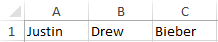
For the convenience of working with text in Excel, there are text functions. They make it easy to process hundreds of lines at once. Let’s consider some of them on examples.
Examples with TEXT function in Excel
This function converts numbers to string in Excel. Syntax: value (numeric or reference to a cell with a formula that gives a number as a result); Format (to display the number in the form of text).
The most useful feature of the TEXT function is the formatting of numeric data for merging with text data. Excel «doesn’t understand» how to display numbers without using the function. The program just converts them to a basic format.
Let’s see an example. Let’s say you need to combine text in string with numeric values:
Using an ampersand without a function TEXT produces an inadequate result:
Excel returned the sequence number for the date and the general format instead of the monetary. The TEXT function is used to avoid this. It formats the values according to the user’s request.
The formula «for a date» now looks like this:
The second argument to the function is the format. Where to take the format line? Right-click on the cell with the value. Click on «Format Cells». In the opened window select «Custom». Copy the required «Type:» in the line. We paste the copied value in the formula.
Let’s consider another example where this function can be useful. Add zeros at the beginning of the number. Excel will delete them if you enter it manually. Therefore, we introduce the formula:
If you want to return the old numeric values (without zeros), then use the «—» operator:
Note that the values are now displayed in numerical format.
Text splitting function in Excel
Individual functions and their combinations allow you to distribute words from one cell to separate cells:
- LEFT (Text, number of characters) displays the specified number of characters from the beginning of the cell;
- RIGHT (Text, number of characters) returns a specified number of characters from the end of the cell;
- SEARCH (Search text, range to search, start position) shows the position of the first occurrence of the searched character or line while viewing from left to right.
The line takes into account the position of each character when dividing the text. Spaces show the beginning or the end of the name you are looking for.
We will split the name, surname and patronymic name into different columns using the functions.
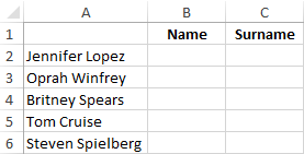
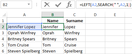
The first line contains only the first and last names separated by a space. Formula for retrieving the name:
The function SEARCH is used to determine the second argument of the LEFT function (the number of characters). It finds a space in cell A2 starting from the left.
For a name, we use the same formula:
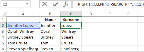
Excel determines the number of characters for the RIGHT function using the SEARCH function. The LEN function «counts» the total length of the text. Then the number of characters up to the first space (found by SEARCH) is subtracted.
The formula for extracting the surname:
Next formulas for extracting the surname is a bit different:
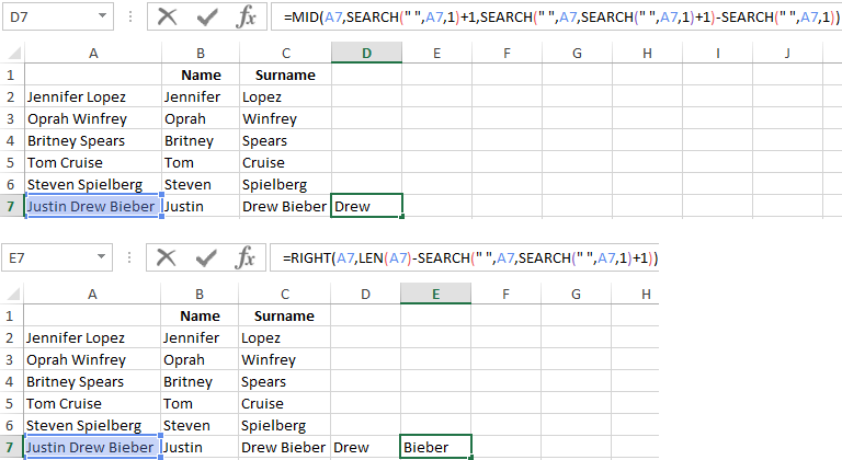
These are five signs on the right. Embedded SEARCH functions search for the second and third spaces in a string. SEARCH («»;A7;1) finds the first space on the left (before the patronymic name). Add one (+1) to the result. We get the position with which we will search for the second space.
Part of the formula SEARCH(» «;A7;SEARCH(» «;A7;1)+1) finds the second space. This will be the final position of the patronymic.
Then the number of characters from the beginning of the line to the second space is subtracted from the total length of the line. The result is the number of characters to the right that you need to return.
Function for merging text in Excel
Use the ampersand (&) operator or the CONCATENATE function to combine values from several cells into one line.
For example, the values are located in different columns (cells):
Put the cursor in the cell where the combined three values will be. Enter «=». Select the first cell and click on the keyboard «&» sign. Then enter the space character enclosed in quotation marks (» «). Enter again «&». Therefore, sequentially connect cells with symbols and spaces.
We get the combined values in one cell:
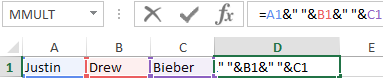
Using the CONCATENATE function:
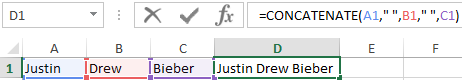
You can add any sign or string to the final expression using quotation marks in the formula.
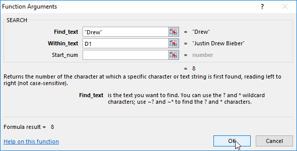
Text SEARCH function in Excel
The SEARCH function returns the starting position of the searched text (not case sensitive). For example:
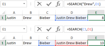
The SEARCH returned to position 8 because the word «Drew» begins with the tenth character in the line. Where can this be useful?
The SEARCH function determines the position of the character in the string line. And the MID function returns symbols values (see the example above). Alternatively, you can replace the found text with the REPLACE.
Download example TEXT functions
The syntax of the SEARCH function:
- «Find_text» is what you need to find;
- «Withing_text» is where to look;
- «Start_num» is from which position to start searching (by default it is 1).
Use the FIND if you need to take into account the case (lower and upper).
Purpose
Convert a number to text in a number format
Return value
A number as text in the given format.
Usage notes
The TEXT function returns a number formatted as text, using the number format provided. You can use the TEXT function to embed formatted numbers inside text.
The TEXT function takes two arguments, value and format_text. Value is the number to be formatted as text and should be a numeric value. If value is already text, no formatting is applied. Format_text is a text string that contains the number formatting codes to apply to value. Supply format_text as a text string enclosed in double quotes («»). To see examples of various number format codes, see Excel Custom Number Formats.
Note: The output from TEXT is always a text string. To format a number and maintain the numeric value, apply regular number formatting.
The TEXT function is useful when concatenating a formatted number to a text string. For example, «Sales last year increased by over $43,500», where the number 43500 has been formatted with a currency symbol and thousands separator. Without the TEXT function, the number formatting will be stripped. This is especially problematic with dates, which appear as large serial numbers. With the TEXT function, you can embed a number in text using exactly the number format needed.
Examples
With the date July 1, 2021 in cell A1, the TEXT function can be used like this:
=TEXT(A1,"dd-mmm-yy") // returns"1-Jul-2021"
=TEXT(A1,"mmmm d") // returns "July 1"
With the number 0.537 in cell A1, TEXT can be used to apply percentage formatting like this:
=TEXT(A1,"0.0%") // returns "53.7%"
=TEXT(A1,"0%") // returns "54%"
The TEXT function is especially useful when concatenating a number to a text string with formatting. For example, with the date July 1, 2021 in cell A1, concatenation causes date formatting to be removed, since dates are numeric values:
="The date is "&A1 // returns "The date is 44378"
The TEXT function can be used to apply date formatting in the final result:
="The date is "&TEXT(A1,"mmmm d") // returns "The date is July 1"
Notes
- Value should be a numeric value
- Format_text must appear in double quotation marks.
- The TEXT function can be used with custom number formats
The TEXT excel function converts a number to a text string based on the format specified by the user. This format is supplied as an argument to the TEXT function. Since the resulting outputs are text representations of numbers, they cannot be used as is in formulas. Therefore, it is recommended to retain the original numbers and create a separate row or column for the converted numbers.
For example, the formula “=TEXT(“10/2/2022″,”mmmm dd, yyyy”)” returns February 10, 2022. Exclude the beginning and ending double quotation marks while entering this formula in Excel.
The purpose of using the TEXT function in Excel is to display a number in the desired format. Since this function also helps combine numbers with other text strings, it tends to make the output more legible. The TEXT function is particularly used when the number formats of different datasets need to be made identical.
Estimated reading time: 21 minutes
Table of contents
- What is Text Function in Excel?
- Syntax of the TEXT Function of Excel
- How to Use the TEXT Function in Excel?
- Example #1–Prefix the Text Strings to the Newly Formatted Date Values
- Example #2–Join the Newly Formatted Time and Date Values
- Example #3–Extract a Mobile Number from its Scientific Notation
- Example #4–Prefix a Text String to the Initially Formatted Monetary Value
- Date Formats of Excel
- Frequently Asked Questions
- TEXT Function in Excel Video
- Recommended Articles
Syntax of the TEXT Function of Excel
The syntax of the TEXT function of Excel is shown in the following image:
The TEXT function of Excel accepts the following arguments:
- Value: This is the number to be converted to a text string. Apart from a number, a date, time or cell reference can also be supplied to the TEXT excel function. The cell reference can contain either a number or an output of another function which can be a number or date.
- Format_text: This is the format to be applied to the “value” argument. It is also called the format code. It is entered within double quotation marks in the TEXT formula of Excel. For instance, “0.00,” “dd/mm/yyyy,” “hh:mm:ss,” and so on are format codes.
Both the stated arguments are mandatory.
Note 1: The format code “0.00” displays a number with two decimal places. In the format code “dd/mm/yyyy,” “dd,” “mm,” and “yyyy” are the notations for days (in two digits), months (in two digits), and years (in four digits) respectively.
Likewise, “hh,” “mm,” and “ss” are the notations for hours (in two digits), minutes (in two digits), and seconds (in two digits) respectively.
For the meaning of the different date formats, refer to the heading “date formats of Excel” given after example #4 of this article.
Note 2: The TEXT function is categorized as a Text/String function of Excel. The TEXT function is available in all versions of Excel.
How to Use the TEXT Function in Excel?
Let us consider some examples to understand the working of the TEXT function in Excel.
Example #1–Prefix the Text Strings to the Newly Formatted Date Values
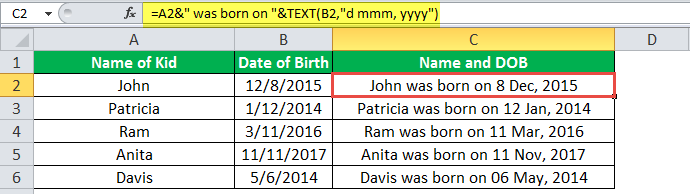
The following table shows the names of five children along with the dates they were born on. The dates are currently in the format m/d/yyyy. Consider the two columns and six rows of the table as columns A and B and rows 1 to 6 of Excel.
We want to perform the following tasks:
- Join the name and date of birth of row 2 by using the ampersand operator. There should not be any space between the joined values.
- Convert each date to the format “dd mmm, yyyy.” Prefix the child’s name and the string “was born on” to each date.
- Show the output when the date of row 2 is in the format “d mmm, yyyy.” Let the prefixes of the preceding point stay as it is.
- Show the date formats “dd mmm, yyyy” (in cell C2) and “d mmm, yyyy” (in cell C6) in a single column.
Explain the outputs obtained in the second and fourth bullet points. Use the TEXT function of Excel.
| Name of Kid | Date of Birth |
|---|---|
| John | 12/8/2015 |
| Patricia | 1/12/2014 |
| Ram | 3/11/2016 |
| Anita | 11/11/2017 |
| Davis | 5/6/2014 |
The steps to perform the given tasks by using the TEXT function of Excel are listed as follows:
Step 1: Enter the following formula in cell C2. Exclude the beginning and ending double quotation marks while entering the given formula.
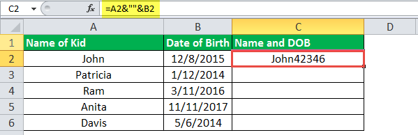
“=A2&“”&B2”
This formula (shown in the image of step 2) joins the values of cells A2 and B2 without any spaces in-between.
Note: The ampersand operator (&) helps join the values of two or more cells. It is called the concatenation operator and is used as an alternative to the CONCATENATE function of Excel. There is no limit on the number of cell values that the ampersand can join.
Step 2: Press the “Enter” key. The output appears in cell C2, as shown in the following image.
Notice that Excel has joined the values of cells A2 and B2 without any spaces in-between. However, the output is not in a readable format. The reason is that the date (12/8/2015) has been converted to a sequential number. The number 42346 represents the date December 8, 2015.
Note: A date is stored in Excel as a sequential or a serial number. This is because a serial number makes it easy to perform calculations. To view the serial number of a date, refer to the “note” preceding step 3 of example #2.
Step 3: To apply the format “dd mmm, yyyy” and insert the stated prefixes, enter the following formula in cell C2.
“=A2&” was born on “&TEXT(B2,”dd mmm, yyyy”)”
Press the “Enter” key. Then, drag the formula of cell C2 till cell C6 by using the fill handle. The outputs are displayed in the following image.
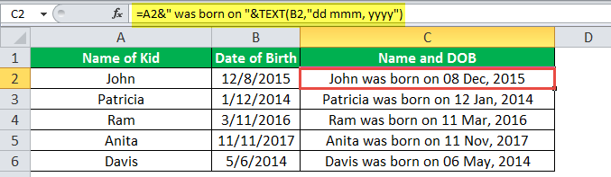
Explanation of the outputs: In column C of the preceding image, the child’s name (in column A) and the text string (was born on) have been prefixed to each date of column B. Since the date is in a suitable format, the output is readable now.
The joined values (outputs) of column C are in the form of statements that are easier to understand than the single values of columns A and B.
Notice that, to insert spaces as the separators in the output, we have inserted spaces at the relevant places in the formula of step 1. Moreover, a comma has also been inserted after the notation of months (mmm). This comma can be seen in each date of the output (in column C).
Step 4: To see the output when the date format is “d mmm, yyyy” and the prefixes are in place, enter the following formula in cell C2.
=A2&” was born on “&TEXT(B2,”d mmm, yyyy”)
Press the “Enter” key. The output appears in cell C2, as shown in the following image.
Notice that the leading zero before the date 8 Dec, 2015 (in cell C2) has disappeared. This zero was there in cell C2 of the preceding image. It has disappeared because, in the current format code, the number of days is represented by a single “d.”
A single “d” omits the leading zeros when the number of days is in a single digit.
Step 5: The outputs obtained after applying different date formats in the same column (column C) are shown in the following image.
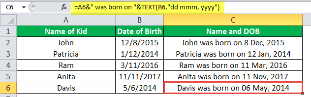
Explanation of the outputs: Notice that in the preceding image, the date of cell C2 is in the format “d mmm, yyyy” while that of cell C6 is in the format “dd mmm, yyyy.” The only difference between these two date formats is in the number of days. The leading zero is absent in cell C2 and present in cell C6.
Hence, with the TEXT function of Excel, one can have different date formats in different cells of the same column. Remember that a format code changes only the appearance of a value; it does not change the value itself. One can create a format code depending on the requirement.
Example #2–Join the Newly Formatted Time and Date Values
The following table shows the times and dates in two separate columns. Consider these columns as columns A and B of Excel. We want to perform the following tasks:
- Join (concatenate) each time value with the respective date. Use the ampersand operator (&) and ensure that there is no space between the two values.
- Show how to copy the formats “h:mm:ss am/pm” and “m/d/yyyy” from the “format cells” window. Convert each time to the former and date to the latter format.
- Join the converted time and date values with the ampersand operator (&). Ensure that there is a space between the two values.
- Show the output when the date format is not enclosed within double quotation marks.
Explain the outputs obtained in the first and third bullet points. Use the TEXT function of Excel for the given tasks.
| Time | Date |
|---|---|
| 7:00:00 AM | 6/19/2018 |
| 7:15:00 AM | 6/19/2018 |
| 7:30:00 AM | 6/19/2018 |
| 7:45:00 AM | 6/19/2018 |
| 8:00:00 AM | 6/19/2018 |
| 8:15:00 AM | 6/19/2018 |
| 8:30:00 AM | 6/19/2018 |
| 8:45:00 AM | 6/19/2018 |
The steps to perform the given tasks by using the TEXT function of Excel are listed as follows:
Step 1: Enter the following formula (without the beginning and ending double quotation marks) in cell C2.
“=A2&“”&B2”
This formula is shown in the image of step 2. It joins the values of cells A2 and B2 without a space in-between.
Step 2: Press the “Enter” key. Then, drag the formula of cell C2 till cell C9 by using the fill handle. The fill handle is displayed at the bottom-right side of cell C2.
The outputs are shown in the following image.
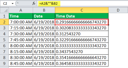
Explanation of the outputs: In column C, the number 43270 (at the end) is the same throughout the range C2:C9. This is the serial number for the date June 19, 2018. The entire decimal number preceding this serial number is the time. So, the decimal number 0.2916667 (in cell C2) represents the time 7:00:00 am.
The outputs obtained in column C of the preceding image are not readable. The reason is that Excel has converted the times (of column A) to decimal numbers and dates (of column B) to sequential numbers. Moreover, joining the decimals with sequential numbers has made the outputs more complicated.
To be able to read the output, it needs to be converted to the relevant format codes. This conversion is shown further in this example.
Note: Excel stores dates as sequential (or serial) numbers and times as decimal numbers. Excel considers a time value as a part of a day. To view the number representing the date, perform the following actions:
- Select any cell of the range B2:B9.
- Press the keys “Ctrl+1” together. The “format cellsFormatting cells is an important technique to master because it makes any data presentable, crisp, and in the user’s preferred format. The formatting of the cell depends upon the nature of the data present.read more” window opens.
- Select “general” under “category” in the “number” tab.
The serial number can be seen under “sample.” Click “cancel” to close the “format cells” window or “Ok” to change the date to a serial number.
Likewise, the decimal number representing the time can also be seen by selecting any cell of the range A2:A9 and following actions “b” and “c” listed above.
Step 3: To convert the time and date values to a readable format, let us first copy the format codes from the “format cells” window. So, select cell C2 and press the keys “Ctrl+1” together.
The “format cells” window opens, as shown in the following image. From the “number” tab, select “custom” under “category. Excel provides a list of formats under “type.”
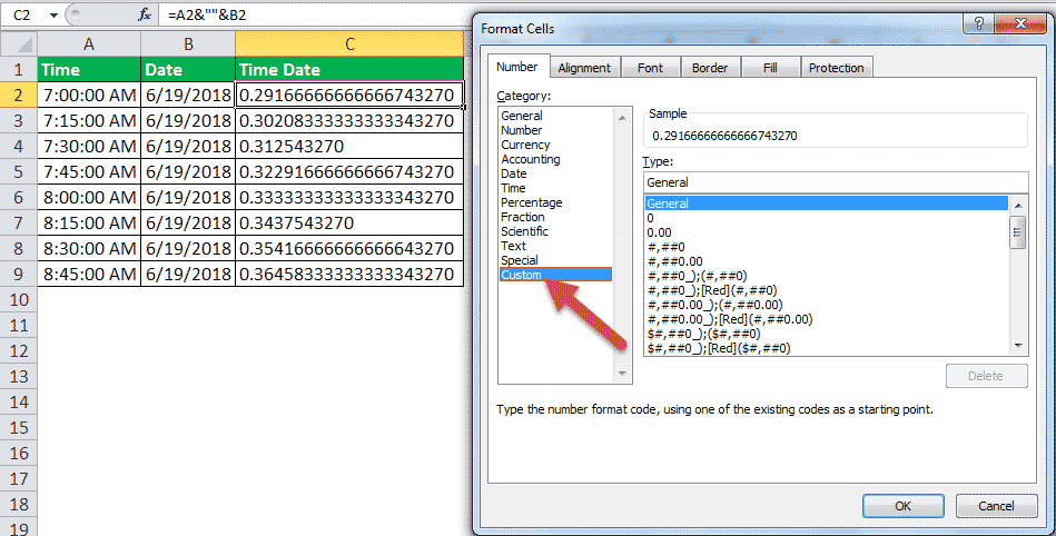
Step 4: Scroll down the list of formats given under “type.” Copy the format “h:mm:ss am/pm.” To copy, just select the format code and press the keys “Ctrl+C.”
The format code is shown in the following image. Once the format has been copied, close the “format cells” window.

Step 5: Copy the format code “m/d/yyyy” for converting the date values. This format code is also available under “type,” as shown in the following image.
Close the “format cells” window after copying the mentioned format code.

Step 6: To apply the new formats to the time and date values and join the resulting values, enter the following formula in cell C2.
“=TEXT(A2,”h:MM:SS AM/PM”)&” “&TEXT(B2,”m/d/yyyy”)”
This formula is shown in the image of step 7. If the format codes have been copied in the preceding steps, they can be pasted at the relevant places in the formula by pressing the shortcut “Ctrl+V.”
According to this formula, the time and date values of cells A2 and B2 are formatted as per the codes “h:MM:SS AM/PM” and “m/d/yyyy” respectively. The formatted (or converted) values are then joined with the ampersand operator.
Notice that in the formula, a space has also been entered within a pair of double quotation marks (like &“ ”&). This space will be inserted in the output at exactly that place where it has been entered in the formula.
Step 7: Press the “Enter” key after entering the TEXT formula. Drag the formula of cell C2 till cell C9.
The outputs are shown in the following image.
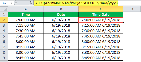
Explanation of the outputs: The time and date values of columns A and B have been converted to the relevant formats in column C. The time values display the hours (h) in a single digit, minutes (mm) in two digits, and seconds (ss) also in two digits. Since all the time values belong to the period before noon, they display “am” at the end.
Likewise, the dates display the months (m) in a single digit, days (d) in a single digit, and years (yyyy) in four digits.
Notice that there is a space between the two joined values in column C. Even though we copied the code “h:mm:ss am/pm” (in step 4) and pasted “h:MM:SS AM/PM” (in step 6), we obtained the correct outputs in column C (in step 7). This is because the format codes are not case-sensitive, implying that “mm” is treated the same as “MM.”
Step 8: To see what happens when the format code for date is entered without the double quotation marks, type the following formula in cell C9.
“=TEXT(A2,”h:MM:SS AM/PM”)&” “&TEXT(B2,m/d/YYYY)”
Press the “Enter” key. Excel returns the “#NAME?” error, as shown in the following image. Therefore, for the TEXT excel function to work, the format code should necessarily be enclosed within double quotation marks.
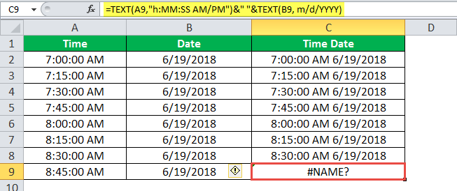
There are two images titled “image 1” and “image 2.” The following information is given:
- Image 1 shows a number having eleven 9s in cell B2. When 1 is added to this number, its digits increase to 12. Excel displays the resulting 12-digit number (in cell B3) in a scientific notation.
- Image 2 shows the names of some people (in column A) and their random mobile numbers in a scientific notation (in column B). The formula bar shows the mobile number of person A. Each mobile number consists of twelve digits, which includes a 2-digit country code at the beginning.
Note that a scientific notationIn Excel, scientific notation is a specific style of writing numbers in scientific and exponential forms. Scientific notation compactly helps display values, allowing us to compare and use the same in calculations.read more (or scientific format) often displays very large or very small numbers in a contracted form. We want to perform the following tasks:
- Display the entire 12-digit mobile number without any spaces in-between.
- Separate the country code from the rest of the number with the help of a hyphen.
Use the TEXT function of Excel for the given tasks.
Image 1
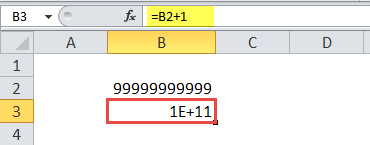
Image 2
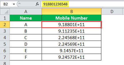
The steps to perform the given tasks by using the TEXT function of Excel are listed as follows:
Step 1: Enter the following formula in cell D2.
“=TEXT(B2,”############”)”
This formula is shown in the formula bar of the succeeding image. Notice that there are 12 hashes in the formula, which represent the 12 digits of a mobile number.
Step 2: Press the “Enter” key. The output appears in cell D2. To obtain the outputs for the entire column D, drag the formula of cell D2 to cell D7. Use the fill handle of cell D2 (displayed at the bottom-right corner) for dragging.
The outputs of column D are shown in the succeeding image.
Note: The output is displayed (in column D) only when one enters a mobile number as an input (in column B) which is converted automatically (or manually) to a scientific format of Excel. In case, a scientific format is typed manually in column B; it cannot be converted to a mobile number of column D.
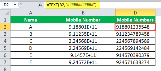
Step 3: To separate the country codes from the rest of the number by using a hyphen, enter the following formula in cell D2.
“=TEXT(B2,“##-##########”)”
Press the “Enter” key. Next, drag the formula of cell D2 till cell D7 with the help of the fill handle. The formula of cell D2 and the outputs are shown in the following image.
Notice that in the formula, the hyphen is placed exactly where it is required in the output. Since only the first two digits of each mobile number are to be separated, the hyphen is placed after two hashes of the formula.

Example #4–Prefix a Text String to the Initially Formatted Monetary Value
There are two images titled “image 1” and “image 2.” The following information is given:
- Image 1 shows the gross profit, expenses, and net profit of an organization. All these numbers are in dollars.
- Image 2 shows how the net profit has been computed. To calculate the net profit, the expenses have been subtracted from the gross profit.
We want to perform the following tasks:
- Show the output when the string “the net profit is” is prefixed to the amount of net profit. Use the ampersand operator for this purpose.
- Prefix the string “the net profit is” to the amount of net profit by using the ampersand. Ensure that in the output, the amount of net profit displays the dollar sign ($) and the comma at the correct places (like $52,291). Use the TEXT function of Excel for this purpose.
Explain the output obtained at the end.
Image 1
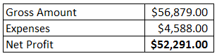
Image 2
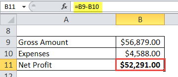
The steps to perform the given tasks are listed as follows:
Step 1: Enter the following formula in cell A13.
“=”The net profit is “&B11”
Exclude the beginning and ending double quotation marks of the formula while entering it in Excel. This formula is shown in the image of step 2.
The given formula prefixes the string “the net profit is” to the value of cell B11. The ampersand helps join the stated string to the amount of net profit (in cell B11).
Step 2: Press the “Enter” key. The output appears in cell A13, as shown in the following image.
Notice that the dollar sign and the comma of the net profit amount (shown in cell B11) have been omitted in the output. Though the string “the net profit is” has been correctly prefixed. The spaces have also been inserted at the right places in cell A13.
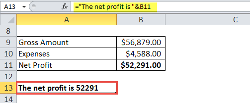
Step 3: To retain the dollar sign and the comma of the amount, enter the following formula in cell A13.
“=”The net profit is ” &TEXT(B11,”$#,##0.00″)”
Press the “Enter” key. The formula and the output are shown in cell A13 of the following image.
Notice that by mistake, a space has been inserted before the ampersand in the formula. However, even then, the correct output has been obtained in cell A13.
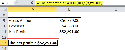
Explanation of the output: This time, the amount of net profit has been properly written (including the dollar sign and the comma) in cell A13. The reason is that the amount of net profit has been converted to the appropriate format in addition to being prefixed by a text string.
So, with the TEXT function of Excel, one can join a number with any string and, at the same time, retain the initial formatting of the number.
Date Formats of Excel
The different format codes for dates have been described as follows:

Frequently Asked Questions
1. Define the TEXT function in Excel with the help of an example.
The TEXT function in Excel helps convert a numerical value to a text string. The conversion is carried out according to the format specified by the user. Once converted, the numerical value becomes a text representation of a number.
The formula “=TEXT(“2/12/2021”,“dddd-mmmm-yyyy”)” converts the date 2/12/2021 to Thursday-December-2021. Ensure that the beginning and ending double quotation marks are excluded while entering this TEXT formula in Excel.
Note: For the working of the TEXT function of Excel, refer to the examples of this article.
2. Why is the TEXT function used in Excel?
The TEXT function is used in Excel for the following reasons:
• It helps convert a numerical value to a text string having a new format.
• It eases joining a numerical value with a text string.
• It helps retain the format of the existing numerical value after concatenation (joining).
• It makes the date or time values given in sequential or decimal numbers more readable and understandable for the users.
• It helps add the leading zeros to a number.
• It allows inserting specific characters (like +,-,(),<>,: etc.) in the output.
Note: The different characters that can be entered in the TEXT formula are the plus (+), minus (-), equal to (=), parentheses (), less than and greater than signs <>, colon (:), apostrophe (‘), curly braces {}, caret (^), forward slash (/), ampersand (&), space ( ), tilde (~), and an exclamation point (!).
The characters should be entered in the format code. These characters are displayed at exactly those places (in the output) where they have been entered in the format code.
3. How is the TEXT function used to add the leading zeros to a number in Excel?
The steps to add the leading zeros to a number are listed as follows:
a. Type “=TEXT” followed by the opening parenthesis.
b. Enter the number as the “value” argument.
c. Enter those many zeros in the format code as the number of digits required in the output.
d. Close the parenthesis and press the “Enter” key.
The leading zeros are added to the number entered in step “b.”
For instance, if the number 148 should appear as a 5-digit number, enter the formula “=TEXT(“148”,“00000”)” without the beginning and ending double quotation marks. It returns 00148.
TEXT Function in Excel Video
Recommended Articles
This has been a guide to the TEXT function of Excel. Here we discuss how to use the TEXT function in Excel along with step-by-step examples. You may also look at these useful functions of Excel–
- Separate Text in ExcelThe methods used to separate text in Excel are as follows: 1) Text to Column (Delimited and Fixed Width) 2) Using Excel Formulasread more
- Add Formula Text in ExcelText in Excel Formula allows us to add text values to using the CONCATENATE function or the ampersand (&) symbol.read more
- INDIRECT in MS Excel
- Trim FunctionThe Trim function in Excel does exactly what its name implies: it trims some part of any string. The function of this formula is to remove any space in a given string. It does not remove a single space between two words, but it does remove any other unwanted spaces.read more
What is the Text Function in Excel?
The TEXT function in Excel converts numbers from the numerical format to text format by using formatting codes. We can use it to display numbers as words, including symbols, while maintaining the numeric value. The TEXT function also helps concatenate numbers to formatted text strings or symbols.
Example, =TEXT(A6,”dd mmmm, yyyy”) converts the numerical Date 27-01-2023 into the text format 27 January, 2023
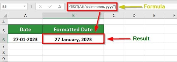
Key Highlights
- We use the TEXT function in Excel to convert Dates into a specific format.
- It does not support a fractional format.
- We use the TEXT function to combine numbers with characters or text.
- We cannot combine the time, Date, #, and 0 in the TEXT function formula.
- Excel gives an error #Name if there are no quotation marks around the argument ‘format_text’.
The Syntax for TEXT Function in Excel
The syntax for the TEXT function is
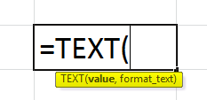
- Value (required): It indicates the numeric value we want to convert to text. The value can be a number, Date, reference to a cell containing a numeric value, or any other function that returns a number or Date.
- format_text (required): It is a format you want to apply. We must provide the argument as format code enclosed in quotation marks, g., “mm/dd/yy”.
How to Use the TEXT Function in Excel?
Consider the following examples to understand the use of the TEXT function:
You can download this TEXT Function Excel Template here – TEXT Function Excel Template
Example #1
Consider the below table, which shows a Date in “dd-mm-yyyy” format. We want to convert it into – “mmmm d, yyyy” using the TEXT function.
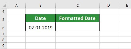
Solution:
Step 1: Place the cursor in cell C6 and enter the formula,
=TEXT(B6,”mmmm d,yyyy”)
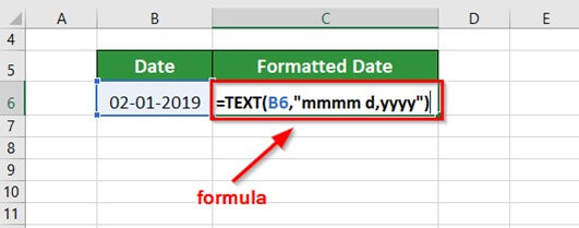
Explanation:
- B6: It is the cell containing an unformatted parameter (Date)
- “mmmm d,yyyy”: The open and closed double quotes indicate the output in text format.
- mmmm: Four times m indicates the month in complete spelling, i.e., January; To write month as only Jan, we need to put it three times, i.e., mmm (refer to the below image)
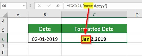
- d: A single d indicates Dates in single digits, i.e., 2
- yyyy: Four times y indicate the year in four digits, i.e., 2019
Step 2: Press Enter key to get the below result
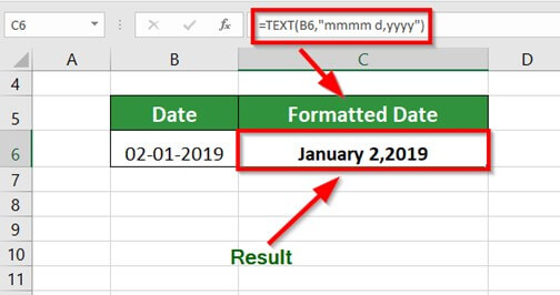
Example #2
The table below shows the time and Dates in columns B and C, respectively. We want the values of the time and Date columns to appear together in column C.
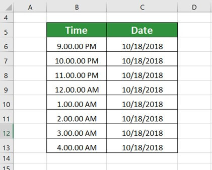
Solution:
Step 1: Place the cursor in cell D6
Note: If we use the CONCATENATE function to combine the values of columns B and C, it gives time in an incorrect format, as seen in the image below. Therefore, we need to use the TEXT function to provide the values in a proper form.
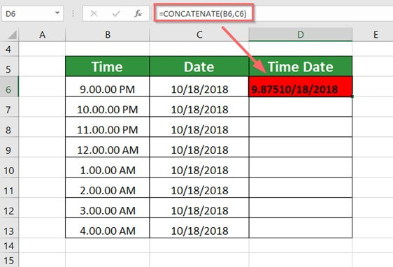
Step 2: Enter the TEXT formula,
=TEXT(B6,”h:mm:ss AM/PM”)& ” “&TEXT(C6,”m/d/yyyy”)
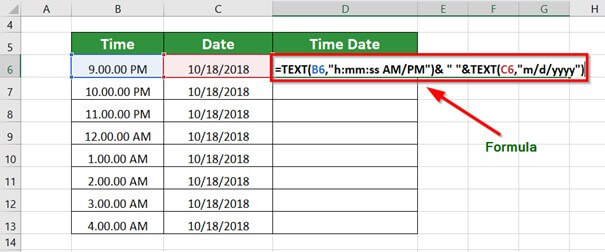
Explanation:
- h:mm:ss AM/PM: It indicates the desired time format
- &” “&: It acts as a separator between the two text
- m/d/yyyy: It indicates the desired Date format
Step 3: Press Enter key to get the below result
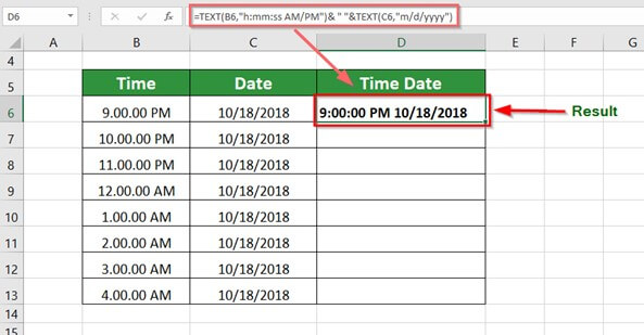
The result is combined time and Date values in single cell D6.
Step 4: Drag the formula in other cells to get the below result
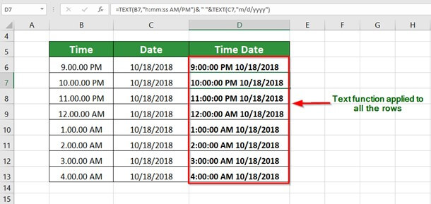
Example #3
The below table shows the scientific notation of a list of mobile numbers with their country codes. We want to use the TEXT function to convert the mobile numbers into the correct and readable format.
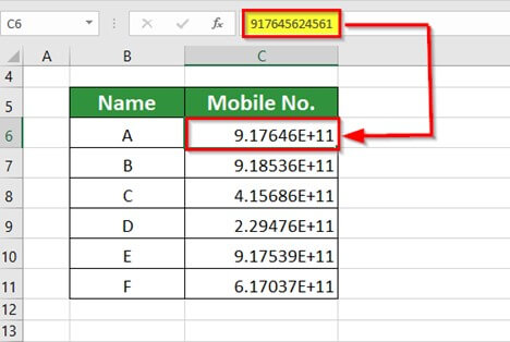
Important: In a Microsoft Excel worksheet, when we enter a value with the number of digits greater than 11, Excel converts that value into a scientific notation in a non-readable format. We can use the TEXT function to convert it into a readable format.
Follow these steps to understand this-
Step 1: Place the cursor in cell D6 and enter the formula,
=TEXT(C6,”############”)
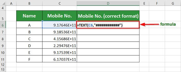
Explanation:
- C6: It is the cell containing the mobile number
- ############: The 12-digit # codes convert numbers in scientific notation into readable format.
Step 2: Press Enter key to get the below result
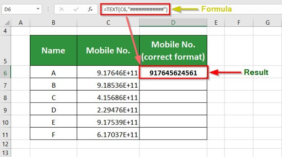
Step 3: Drag the formula in other cells to get the below result
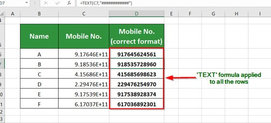
Tip: We can differentiate the country code from the mobile number by inserting a hyphen (-) at the desired location in the Text Formula
So,
Step 4: Modify the formula by inserting a hyphen (-) after two digits in the formula, as shown below,
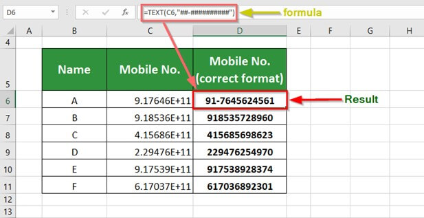
Step 5: Drag the formula in other cells to get the below result
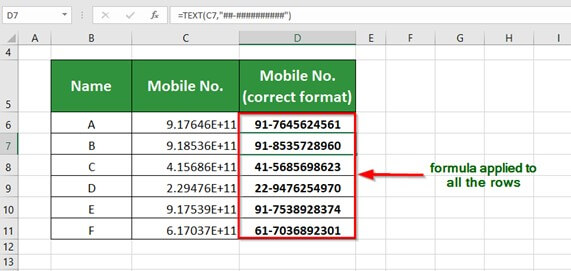
Using Concatenate and Text Function in Excel Together
We want to display the present day and Date using the TEXT function.
Solution:
Place the cursor in cell B5 and enter the formula,
=CONCATENATE(“Today is”,” “, TEXT(TODAY(),”dddd d mmm, yyy”))
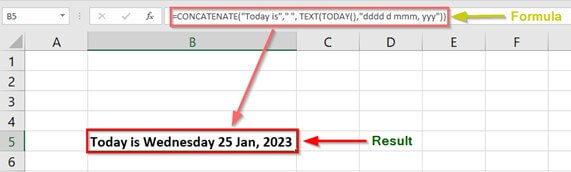
Explanation:
- TODAY(): Indicates the present day of the week
- dddd d mmm, yyy: Indicates the current Date with the day.
The formula combines (concatenates) the text Today is with the present day to give the result- Today is Wednesday 25 Jan, 2023.
How to Get the Format Codes for Text Function in Excel?
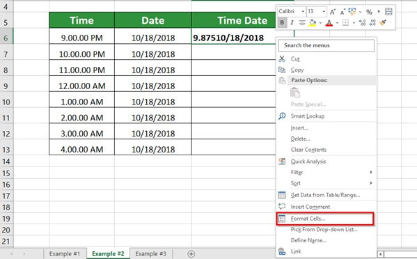
To locate the format codes for time:
Right-click the desired cell > Go To Format Cells > Number > Custom > Select the desired time Type from list > OK.
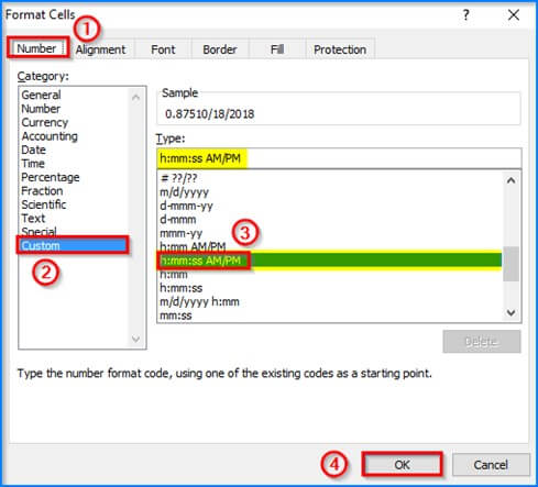
To locate the format codes for the Date:
Right-click the desired cell > Go To Format Cells > Number > Custom > Select the desired Date Type from the list > OK.
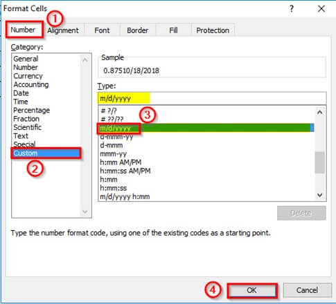
Shortcut: To open Format Cells,
- Press CTRL+1 in windows, and
- +1 in Mac
List of Format Codes for TEXT Function in Excel
The Text function accepts most format codes used in Excel number formats. Below is a table with the most common and frequently used format codes.
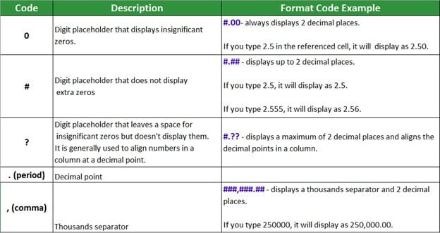
*In addition, we can include any of the below characters in the format code, and they will be displayed as entered.
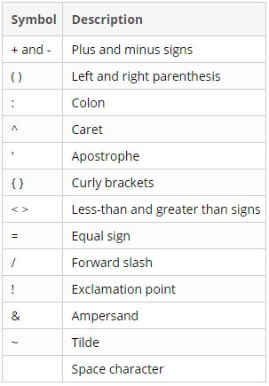
Format Codes used in Excel while dealing with Dates
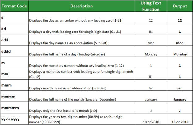
List of Built-in Excel Text Functions
Below is a list of built-in Text functions in Excel with their uses
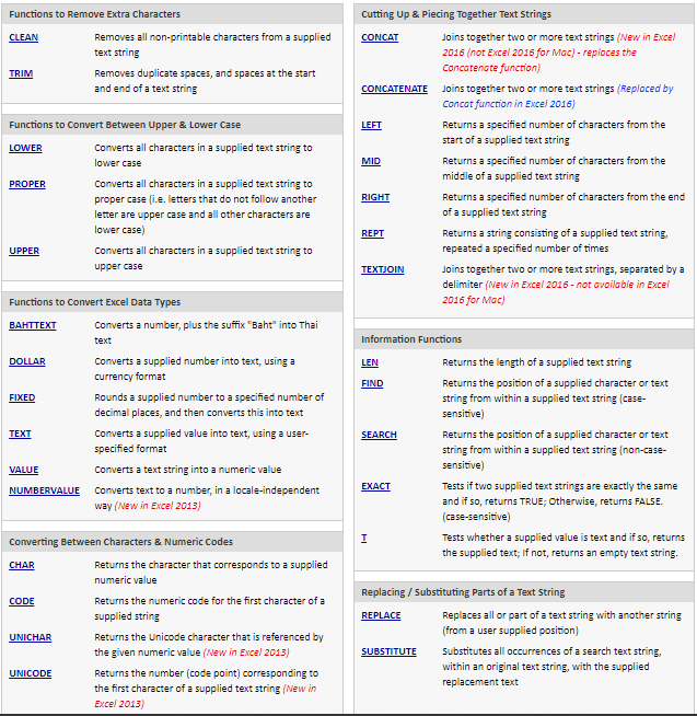
Things to Remember
- The Text function in Excel cannot convert numbers from 123 formats to One Two Three. To do so, we have to use Visual Basics (VBA).
- The Text function converts a numeric value to a formatted text; therefore, we cannot use the result for calculation purposes.
- The ‘format_text’ argument in the text function formula cannot contain an asterisk character (*).
- TEXT function is available in the following versions of Microsoft Excel- Excel for Office 365, Excel 2019, Excel 2016, Excel 2013, Excel 2011 for Mac, Excel 2010, Excel 2007, Excel 2003, Excel XP, and Excel 2000.
Frequently Asked Questions (FAQs)
Q1) What are the arguments of text function?
Answer: The TEXT function takes two arguments- value and format_text.
Value: It is the number we need to format as text. The function will not apply a format code if the argument is already text.
format_text: It is a text string (format) that we want to apply to the value. We must provide the argument in quotation marks to give the correct result.
Q2) How do you use the text function in sheets?
Answer: To use the TEXT function in Google sheets, consider the below example
- Place the cursor in the cell where you want the result
- Type the formula,
=TEXT(A4,”HH mm”)
The formula will convert the time format from 12 Hrs format (4:15:00 PM) to 24 Hrs Format (16 15)
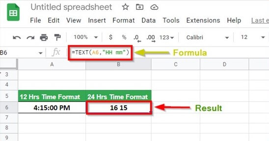
Q3) What is the use of text functions in Excel?
Answer: The TEXT function lets you convert numbers into a more readable format. We can change the appearance of numbers to the desired forms by applying the format codes in Excel.
Q4) How to use text function in excel?
Answer: To understand using the TEXT function, consider the below example,
- Place the cursor in cell B6
- Type the formula,
=TEXT(A6,”0%”)
The formula will convert the decimal 0.565 to the percentage format as 57%.
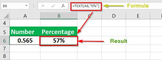
Recommended Articles
The above article is a guide to using Text Function in Excel. To learn about more Excel-related concepts, EDUCBA recommends the below-given articles.
- Excel Text with Formula
- Formatting Text in Excel
- Search For Text in Excel
- VBA Text
- На главную
- Категории
- Программы
- Microsoft Excel
- Работа с текстом в Excel
Microsoft Excel предлагает множество полезных функций, с помощью которых можно легко и быстро обрабатывать различные данные. Однако их применение не ограничивается только числами, они могут быть использованы с ячейками, содержащими текст. Ниже представлены основные функции для работы с текстом.
2020-09-20 08:34:0551

Microsoft Excel предлагает множество полезных функций, с помощью которых можно легко и быстро обрабатывать различные данные. Однако их применение не ограничивается только числами, они могут быть использованы с ячейками, содержащими текст. Ниже представлены основные функции для работы с текстом.

Функция ТЕКСТ в Excel
Преобразовывает числовые значения в текстовые и задает формат отображения посредством специальных строк форматирования. Удобна в тех случаях, когда нужно показать числа в определенном формате или объединить их с текстом, символами.
=ТЕКСТ(числовое_значение_или_формула_в_результате_вычисления_которой_получается_число;формат_ который_требуется_применить_к_указанному_значению)
Для определения формата следует предварительно клацнуть по значению правой кнопкой мышки – и в выпадающем меню выбрать одноименную опцию, либо нажать сочетание клавиш Ctrl+1. Перейти в раздел «Все…». Скопировать нужный формат из списка «Тип».
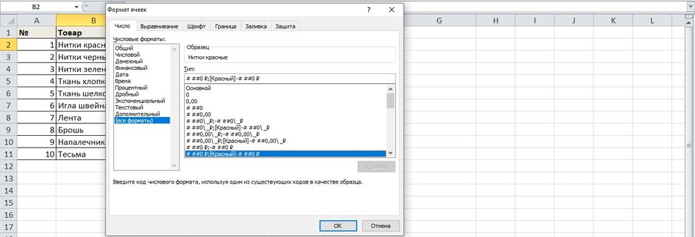
Чтобы понять, как работает функция, необходимо открыть книгу и создать таблицу с данными.
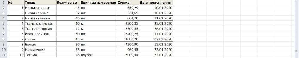
- Кликнуть по любому свободному месту, например, G Ввести знак «=» и ссылку на адрес ячейки – B2. Активировать Мастер функций, нажав на кнопку fx (слева) во вкладке «Формулы», или с помощью комбинации клавиш Shift+F3.
- На экране отобразится окно Мастера. В строке поиска ввести название функции и нажать «Найти».
- В списке нужное название будет выделено синим цветом. Нажать «Ок».
- Указать аргументы: ссылку на число и скопированное значение формата. В строке формулы после B2 вписать знак «&».
- В результате появится сумма в денежном формате вместе с наименованием товара. Протянуть формулу вниз.
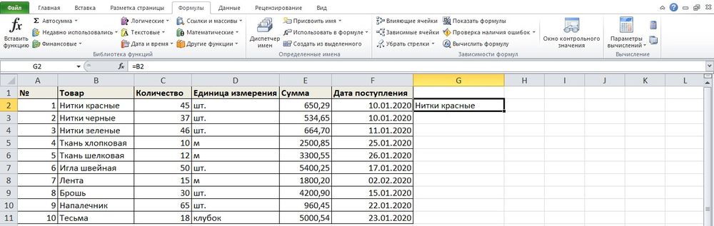
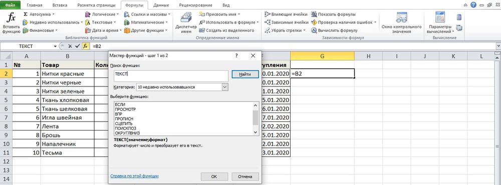
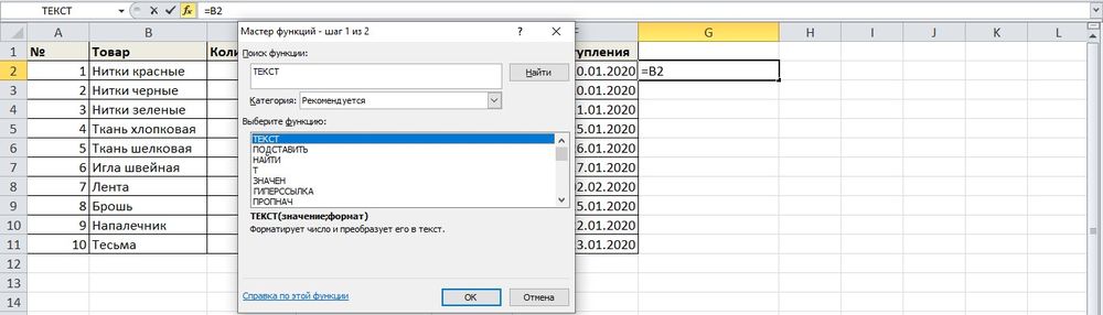
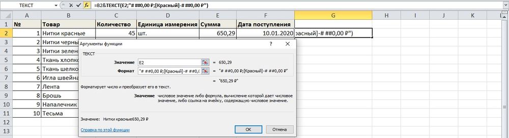
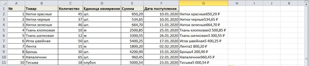
Еще один пример.
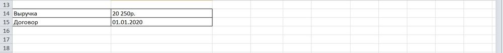
Необходимо объединить текстовые и числовые значения с помощью формулы =A14&» «&»составляет»&» «&B14&»,»&» «&A15&» «&ТЕКСТ(B15;»ДД.ММ.ГГ;@»).
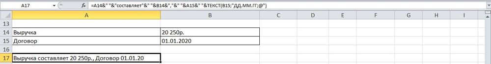
Таким образом любые данные преобразовываются в удобный формат.
Объединение ячеек в Excel
Чтобы объединить ячейки в одну строку без потери данных, можно использовать или знак «&», или функцию СЦЕПИТЬ (в новых версиях – ОБЪЕДИНИТЬ).
=СЦЕПИТЬ(ячейка_1;» «;ячейка_2;» «;ячейка_3;» «)
Пустые кавычки (» «) – это пробел. Без пробелов слова будут отображаться слитно. С помощью кавычек в формулу добавляется любой знак («.» или «,») и текст.
- Следует установить курсор в месте, где будет отображаться готовое значение.
- Написать формулу.
- Нажать «Enter».
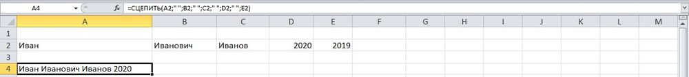
Второй вариант формулы тоже простой: =ячейка1&» «&ячейка2&» «&ячейка3.
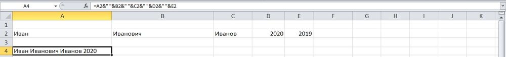
Если в результате строка будет содержать 32767 символов и более, появится ошибка #ЗНАЧ!.
Перенос текста в ячейке в Excel
Перенести текст внутри одной ячейки на следующую строку можно несколькими способами:
- Выделить ячейку и кликнуть по опции «Перенос…», которая расположена во вкладке «Главная».
- Щелкнуть правой кнопкой мышки по выделенной ячейке, в выпадающем меню выбрать «Формат…». В появившемся на экране окне перейти на вкладку «Выравнивание», поставить галочку в поле «Переносить по словам». Сохранить изменения, нажав «Ок».
- При наборе текста перед конкретным словом зажать комбинацию клавиш Alt+Enter – курсор переместится на новую строку.
- С помощью функции СИМВОЛ(10). При этом нужно объединить текст во всех ячейках, а поможет сделать это амперсанд «&»: =A1&B1&СИМВОЛ(10)&A2&B2&СИМВОЛ(10).
- Также вместо оператора «&» можно использовать функцию СЦЕПИТЬ. Формула будет иметь вид: =СЦЕПИТЬ(A2;» «;СИМВОЛ(10);B2;» «;C2;» «;D2;СИМВОЛ(10);E2;СИМВОЛ(10);F2).
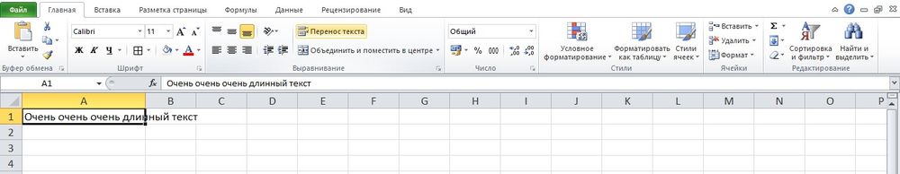
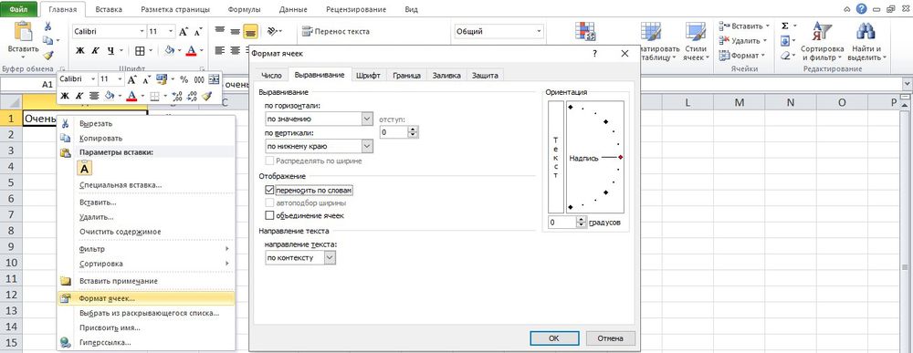
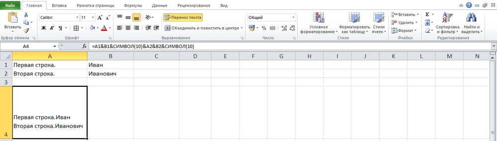
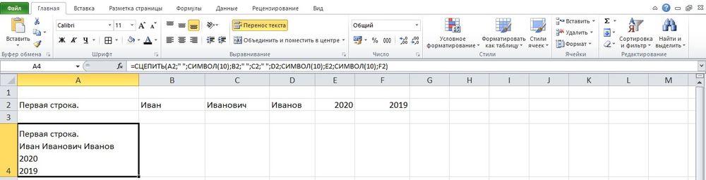
Чтобы перенос строки с использованием формул отображался корректно в книге, следует включить опцию переноса на панели.
Какой бы метод не был выбран, текст распределяется по ширине столбца. При изменении ширины данные автоматически перестраиваются.
Количество символов в ячейке в Excel
При работе с данными иногда требуется посчитать количество символов в определенной ячейке. Вручную делать это неудобно, особенно когда значений много или содержимое меняется в зависимости от заданного условия. Для таких случаев используется функция ДЛСТР.
=ДЛСТР(ячейка_1)
Функция работает только с одним значением.
- Выделить ту ячейку, где будет показан подсчет.
- Вписать формулу, указывая ссылку на адрес определенной ячейки.
- Нажать «Enter».
- Растянуть результат на другие строки или столбцы.
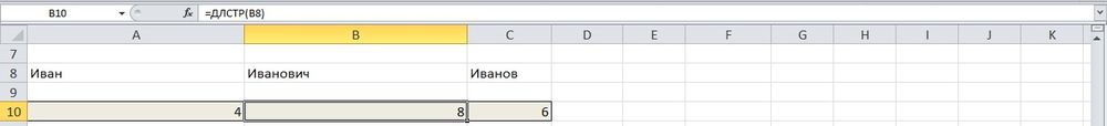
Можно посчитать общее количество символов:
- Выделить все значения, во вкладке «Главная» на панели справа найти инструмент «Сумма».
- Кликнуть по одноименной опции. Рядом (под или с боковой стороны от выделенного диапазона) отобразится результат.
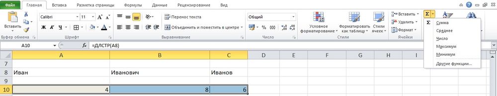
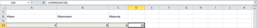
В разбросанных ячейках
В этом случае необходимо воспользоваться ДЛСТР и суммированием:
- Установить курсор в желаемом месте.
- Ввести формулу =ДЛСТР(значение1)+ДЛСТР(значение2)+ДЛСТР(значение3) и т.д.
- Нажать «Enter».
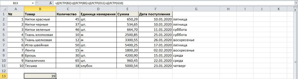
Как преобразовать текст в число
Часто при добавлении новых числовых данных в таблицу они по умолчанию преобразовываются в текст. В итоге не работают вычисления и формулы. В Excel есть возможность сразу узнать, как отформатированы значения: числа выравниваются по правому краю, текст – по левому.
Когда возле значения (в левом углу сверху) есть зеленый треугольник, значит, где-то допущена ошибка. Существует несколько легких способов преобразования:
- Через меню «Ошибка». Если кликнуть по значению, слева появится значок с восклицательным знаком. Нужно навести на него курсор, клацнуть правой кнопкой мышки. В раскрывшемся меню выбрать вариант «Преобразовать в число».
- Используя простое математическое действие – прибавление / отнимание нуля, умножение / деление на единицу и т.п. Но необходимо создать дополнительный столбец.
- Добавив специальную вставку. В пустой ячейке написать цифру 1 и скопировать ее. Выделить диапазон с ошибками. Кликнуть по нему правой кнопкой мышки, из выпадающего меню выбрать «Специальную вставку». В открывшемся окне поставить галочку возле «Умножить». Нажать «Ок».
- При помощи функций ЗНАЧЕН (преобразовывает текстовый формат в числовой), СЖПРОБЕЛЫ (удаляет лишние пробелы), ПЕЧСИМВ (удаляет непечатаемые знаки).
- Применив инструмент «Текст по столбцам» к значениям, которые расположены в одном столбце. Нужно выделить все числовые элементы, во вкладке «Данные» найти указанную опцию. В открывшемся окне Мастера нажимать далее до 3-го шага – проверить, какой указан формат, при необходимости – изменить его. Нажать «Готово».
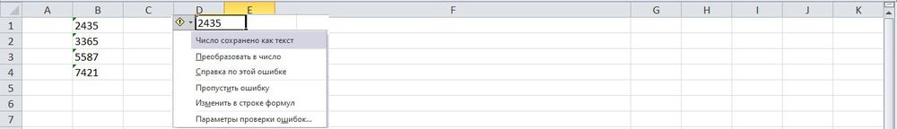
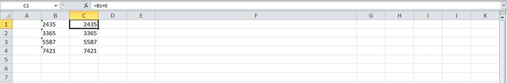
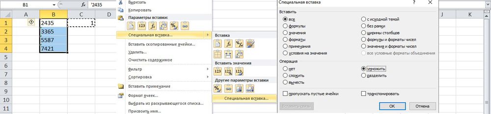
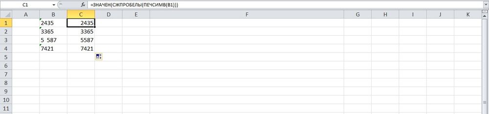
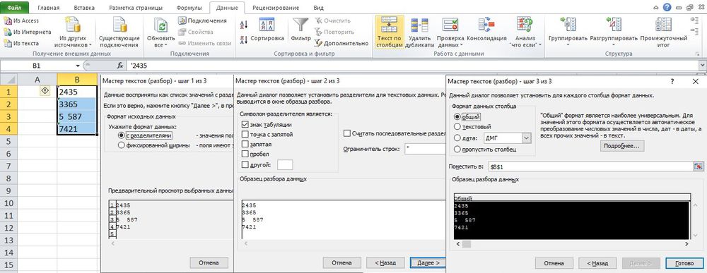
Как преобразовать дату в текст
Функция ТЕКСТ позволяет определить день недели по дате:
- Кликнуть по ячейке.
- Написать формулу =ТЕКСТ(значение;»ДДДД»).
- Нажать «Enter».
- Протянуть формулу вниз до последней даты.
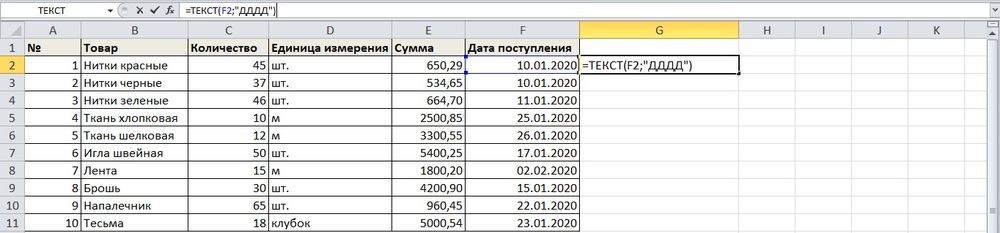
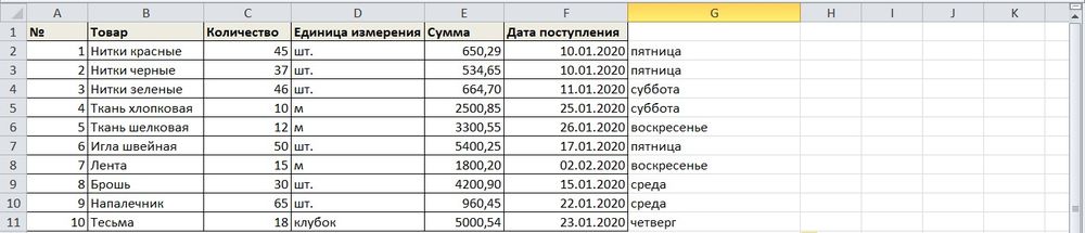
Для представления даты в текстовом виде используется формула =ТЕКСТ(значение;»ДД МММ ГГГГ»).
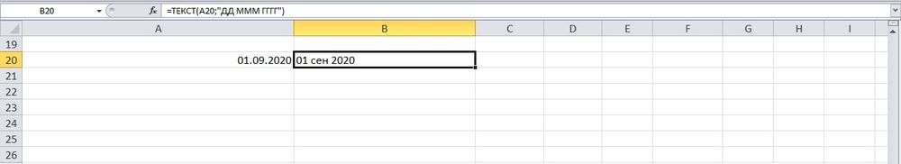
Для отображения даты в аргументе формулы в качестве формата используются следующие коды:
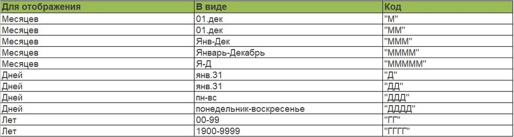

Ваш покорный слуга — компьютерщик широкого профиля: системный администратор, вебмастер, интернет-маркетолог и много чего кто. Вместе с Вами, если Вы конечно не против, разовьем из обычного блога крутой технический комплекс.
На чтение 1 мин
Функция TEXT (ТЕКСТ) в Excel используется для преобразования числа в текстовый формат и отображения его в специальном формате.
Содержание
- Что возвращает функция
- Синтаксис
- Аргументы функции
- Дополнительная информация
- Примеры использования функции ТЕКСТ в Excel
Что возвращает функция
Текст в заданном формате.
Синтаксис
=TEXT(value, format_text) — английская версия
=ТЕКСТ(значение, которое нужно отформатировать; «код формата, который требуется применить») — русская версия
Аргументы функции
- value (значение, которое нужно отформатировать) — число для преобразования в текст;
- format_text (код формата, который требуется применить) — формат для отображения числового значения.
Дополнительная информация
- Это очень полезная функция в тех случаях, когда нужно показать числа в каком-то формате или комбинировать числа и текст. Например, представим, что у нас в ячейке А1 есть число «3333» и нам надо использовать его в тексте «Продажи составили $3,333». В этом нам поможет формула:
=»Продажи составили «&TEXT(A1,»$#,###») — английская версия
=»Продажи составили «&ТЕКСТ(A1;»$#,###») — русская версия
- Числа, преобразованные в текст не могут быть использованы для дальнейших вычислений;
- Если вы хотите использовать числа в формулах/вычислениях, используйте формат числового значения.
Примеры использования функции ТЕКСТ в Excel
