
Содержание
- How to copy only plain text of cells in Excel?
- 9 Answers 9
- How to select cells that only contain Text, Number or Error in Microsoft Excel
- Selecting cells that only contain Text in Excel
- Excel substring: how to extract text from cell
- How to extract substring of a certain length
- Extract substring from start of string (LEFT)
- Get substring from end of string (RIGHT)
- Extract text from middle of string (MID)
- Extract substring before or after a given character
- How to extract text before a specific character
- How to extract text after character
- How to extract text between two instances of a character
- How to find substring in Excel
- How to extract text from cell with Ultimate Suite for Excel
- More formulas for substrings in Excel
- Available downloads
How to copy only plain text of cells in Excel?
I am designing an Excel worksheet where the user will click a command button which copies a predetermined range of cells. The user would then paste the contents into a web app using Firefox or IE. The design of the web app is out of my control and currently the text boxes that are used for data input are rich text inputs. This causes the text to look odd and formatted like Excel when the user pastes into them.
Is there a way in Excel using VBA to copy only the plain text of the cells that are selected? No formatting, no tabling or cell borders, just the text and nothing else. My current workaround macro is copying the cells, opening Notepad, pasting into Notepad, and then copying from Notepad to get the plain text. This is highly undesirable and I’m hoping there’s a way to do this within Excel itself. Please let me know, thanks!
9 Answers 9
Something like this?
Copy copies the entire part, but we can control what is pasted.
Same applies to Range objects as well.
EDIT
AFAIK, there is no straighforward way to copy only the text of a range without assigning it to a VBA object (variable, array, etc.). There is a trick that works for a single cell and for numbers and text only (no formulas):
but most developers avoid SendKeys because it can be unstable and unpredictable. For example, the code above works only when the macro is executed from excel, not from VBA . When run from VBA , SendKeys opens the object browser, which is what F2 does when pressed at the VBA view 🙂 Also, for a full range, you will have to loop over the cells, copy them one by one and paste them one by one to the application. Now that I think better, I think this is an overkill..
Using arrays is probably better. This one is my favorite reference on how you pass ranges to vba arrays and back: http://www.cpearson.com/excel/ArraysAndRanges.aspx
Personally, I would avoid SendKeys and use arrays. It should be possible to pass the data from the VBA array to the application, but hard to say without knowing more about the application..
Источник
How to select cells that only contain Text, Number or Error in Microsoft Excel
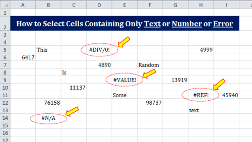
At times you may want to select the cells that have specified type of data in it, by which you can distinguish between cells that contain different types of data, which allows you to delete, fill or lock cells by the data type for various other reasons.
Follow below steps to select cells that only contain Text:
- Press F5 to access Go To window

- In the Go To dialog box, click on Special button

- In the Go To Special dialog box, select Constants. And check only Text


Below are the examples that show how to select cells that only contain Number or Errors:


Bonus Tip:
Use formulas =ISTEXT() =ISNUMBER() =ISERROR() with Conditional Formatting to Highlight the cells that only contain Text, Number or Errors. Check this article for step by step guide to learn Conditional Formatting How to Highlight a Row in Excel Using Conditional Formatting


Now that you know these two nifty techniques and can play around with the options and get various desired results.
Happy Excelling… 🙂
Источник
Selecting cells that only contain Text in Excel
To select specific cells that only contain text, we can use the Go-To option or Conditional Formatting in Excel.
Let’s take an example and understand how and where we can use these functions.
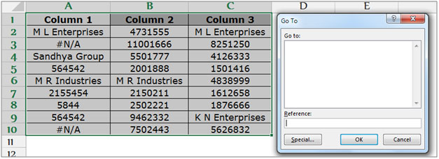
We have data in range A1:C10 which contains text and numbers. We need to select only those cells which contain text.
Lets see how we can use the Go-To Special option.
Go-To Special:- This option is used to quickly re-direct to different cells in Excel.
Shortcut: F5 and Ctrl+G
Command button: Go to Home>click on Find & Select >select Go to Special
Follow the below given steps:-

- Press key F5 on the keyboard, the Go- To dialog box willappear.
- Click on “SPECIAL” button.
- The Go-to Special dialog box will appear.
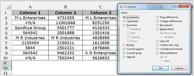
- Click on “Constants”, the inactive links under Formulas will get activated.

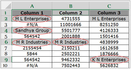
- Now uncheck all the options except “Text” and click on OK, only the cells containing text will be selected.
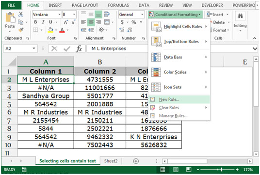
Select the cells containing text by using Conditional Formatting.
- Select the data A1:C10
- Go to the Home tab> in the Styles group > select Conditional Formatting.
- Select New rule from the Conditional Formatting drop down menu.
 ;
;
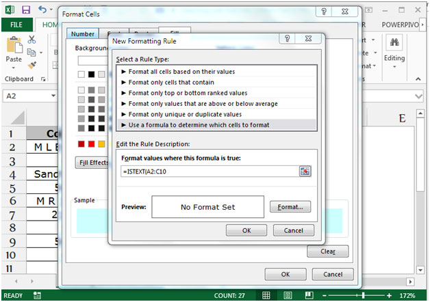
- The New Formatting Rule dialog box will appear.
- Select “Use a formula to determine which cells to format”
- In the formula tab, write the TEXT function.
- =ISTEXT(A2:C10), click on “Format” button.

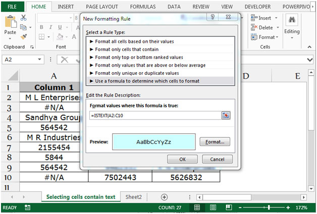
- The Format Cells dialog box will appear.
- Choose any color.
- Click on OK, Format Cells dialog box.
- Click on OK, New Formatting Rule dialog box.
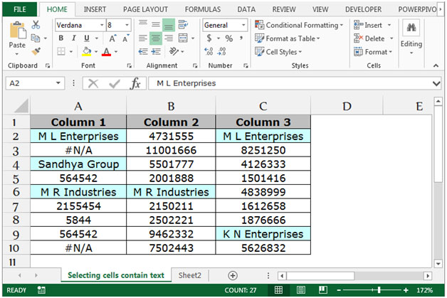
These are the ways in which you can highlight the text contains cells in Microsoft Excel.
Источник
 by Svetlana Cheusheva, updated on March 17, 2023
The tutorial shows how to use the Substring functions in Excel to extract text from a cell, get a substring before or after a specified character, find cells containing part of a string, and more.
Before we start discussing different techniques to manipulate substrings in Excel, let’s just take a moment to define the term so that we can begin on the same page. So, what is a substring? Simply, it’s part of a text entry. For example, if you type something like «AA-111» in a cell, you’d call it an alphanumeric string, and any part of the string, say «AA», would be a substring.
Although there is no such thing as Substring function in Excel, there exist three Text functions (LEFT, RIGHT, and MID) to extract a substring of a given length. Also, there are FIND and SEARCH functions to get a substring before or after a specific character. And, there are a handful of other functions to perform more complex operations such as extracting numbers from a string, replacing one substring with another, looking up partial text match, etc. Below you will find formula examples to do all this and a lot more.
Microsoft Excel provides three different functions to extract text of a specified length from a cell. Depending on where you want to start extraction, use one of these formulas:
- LEFT function — to extract a substring from the left.
- RIGHT function — to extract text from the right.
- MID function — to extract a substring from the middle of a text string, starting at the point you specify.
As is the case with other formulas, Excel substring functions are best to learn from an example, so let’s look at a few ones.
To extract text from the left of a string, you use the Excel LEFT function:
Where text is the address of the cell containing the source string, and num_chars is the number of characters you want to extract.
For example, to get the first 4 characters from the beginning of a text string, use this formula:
=LEFT(A2,4) 
Get substring from end of string (RIGHT)
To get a substring from the right part of a text string, go with the Excel RIGHT function:
For instance, to get the last 4 characters from the end of a string, use this formula:
=RIGHT(A2,4) 
If you are looking to extract a substring starting in the middle of a string, at the position you specify, then MID is the function you can rely on.
Compared to the other two Text functions, MID has a slightly different syntax:
Aside from text (the original text string) and num_chars (the number of characters to extract), you also indicate start_num (the starting point).
In our sample data set, to get three characters from the middle of a string beginning with the 6th character, you use the following formula:
=MID(A2,6,3) 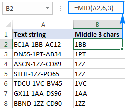
Tip. The output of the Right, Left and Mid formulas is always text, even when you are extracting a number from a text string. If you want to operate on the result as a number, then wrap your formula in the VALUE function like this:
As shown in the above examples, the Left, Right and Mid functions cope nicely with uniform strings. When you are dealing with text strings of variable length, more complex manipulations shall be needed.
Note. In all of the below examples, we will be using the case-insensitive SEARCH function to get the position of a character. If you want a case-sensitive formula, use the FIND function instead.
To get a substring preceding a given character, two things are to be done: first, you determine the position of the character of interest, and then you pull all characters before it. More precisely, you use the SEARCH function to find the position of the character, and subtract 1 from the result, because you don’t want to include the character itself in the output. And then, you send the returned number directly to the num_chars argument of the LEFT function:
For example, to extract a substring before the hyphen character (-) from cell A2, use this formula:
No matter how many characters your Excel string contains, the formula only extracts text before the first hyphen: 
To get text following a specific character, you use a slightly different approach: get the position of the character with either SEARCH or FIND, subtract that number from the total string length returned by the LEN function, and extract that many characters from the end of the string.
In our example, we’d use the following formula to extract a substring after the first hyphen:
=RIGHT(A2,LEN(A2)-SEARCH(«-«,A2)) 
To get a substring between two occurrences of a certain character, use the following generic formula:
The first two arguments of this MID formula are crystal clear:
Text is the cell containing the original text string.
Start_num (starting point) — a simple SEARCH formula returns the position of the desired character, to which you add 1 because you want to start extraction with the next character.
Num_chars (number of chars to extract) is the trickiest part:
- First, you work out the position of the second occurrence of the character by nesting one Search function within another.
- After that, you subtract the position of the 1st occurrence from the position of the 2nd occurrence, and subtract 1 from the result since you don’t want to include the delimiter character in the resulting substring.
For example, to extract text surrounded by two hyphens, you’d use this formula:
=MID(A2, SEARCH(«-«,A2) + 1, SEARCH(«-«,A2,SEARCH(«-«,A2)+1) — SEARCH(«-«,A2) — 1)
The screenshot below shows the result: 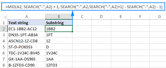
If you are looking to extract text between 2 nd and 3 rd or 3 nd and 4 th occurrences of the same character, you can use a more compact SEARCH SUBSTITUTE combination to get the character’s position, as explained in How to find Nth occurrence of a character in a string:
In our case, we could extract a substring between the 2nd and 3rd hyphens with the following formula:
=MID(A2, FIND(CHAR(1),SUBSTITUTE(A2,»-«,CHAR(1),2))+1, FIND(CHAR(1),SUBSTITUTE(A2,»-«,CHAR(1),3)) — FIND(CHAR(1),SUBSTITUTE(A2,»-«,CHAR(1),2))-1) 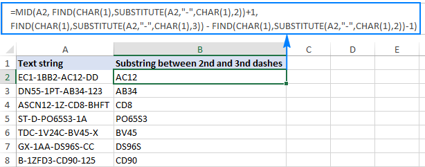
How to find substring in Excel
In situations when you don’t want to extract a substring and only want to find cells containing it, you use the SEARCH or FIND function as shown in the above examples, but perform the search within the ISNUMBER function. If a cell contains the substring, the Search function returns the position of the first character, and as long as ISNUMBER gets any number, it returns TRUE. If the substring is not found, the search results in an error, forcing ISNUMBER to return FALSE.
Supposing, you have a list of British postcodes in column A and you want to find those that contain the substring «1ZZ». To have it done, use this formula:
The results will look something similar to this: 
If you’d like to return your own message instead of the logical values of TRUE and FALSE, nest the above formula into the IF function:
=IF(ISNUMBER(SEARCH(«1zz», A2)), «Yes», «»)
If a cell contains the substring, the formula returns «Yes», an empty string («») otherwise: 
As you may remember, the Excel SEARCH function is case-insensitive, so you use it when the character case does not matter. To get your formula to distinguish the uppercase and lowercase characters, opt for the case-sensitive FIND function.
For more information on how to find text and numbers in Excel, please see If cell contains formula examples.
As you have just seen, Microsoft Excel provides an array of different functions to work with text strings. In case you are unsure which function is best suited for your needs, commit the job to our Ultimate Suite for Excel. With these tools in your Excel’s arsenal, you just go to Ablebits Data tab > Text group, and click Extract: 
Now, you select the source cells, and whatever complex strings they contain, a substring extraction boils down to these two simple actions:
- Specify how many characters you want to get from the start, end or middle of the string; or choose to extract all text before or after a given character.
- Click Insert Results. Done!
For example, to pull the domain names from the list of email addresses, you select the All after text radio button and type @ in the box next to it. To extract the user names, you select the All before text radio button, as shown in the screenshot below. 
And you will get the following results in a moment: 
Apart from speed and simplicity, the Extract Text tool has extra value — it will help you learn Excel formulas in general and substring functions in particular. How? By selecting the Insert as formula checkbox at the bottom of the pane, you ensure that the results are output as formulas, not values.
In this example, if you select cells B2 and C2, you will see the following formulas, respectively:
- To extract username:
=IFERROR(LEFT(A2,SEARCH(«@»,A2)-1),»»)
To extract domain:
=IFERROR(RIGHT(A2, LEN(A2)- SEARCH(«@»,A2) — LEN(«@») + 1),»»)
How much time would it take you to figure out these formulas on your own? 😉
Since the results are formulas, the extracted substrings will update automatically as soon as any changes are made to the original strings. When new entries are added to your data set, you can copy the formulas to other cells as usual, without having to run the Extract Text tool anew.
If you are curious to try this as well as many other useful features included with Ultimate Suite for Excel, you are welcome to download evaluation version.
More formulas for substrings in Excel
In this tutorial, we have demonstrated some classic Excel formulas to extract text from string. As you understand, there can be almost infinite variations of these basic scenarios. Below you will find a few more formula examples where the Text functions come in handy.
- How to extract number from string in Excel — formula examples to get a number from various text strings.
- How to extract Nth word from a text string — how to use MID in combination with 4 other functions to get any Nth word from a cell.
- How to extract a word containing a certain substring — one more non-trivial MID formula that pulls a word containing a specific character(s) from anywhere in the source string.
- How to extract text between parentheses — using this approach, you can get a substring between any two characters you specify.
- How to Lookup partial string match — how to use an Excel substring function (LEFT, RIGHT or MID) in combination with Vlookup to retrieve values based on partial match.
- How to replace one substring with another — a formula to find and replace a certain character or substring within the text string.
- How to count cells containing a substring — how to use the COUNTIF function with wildcard characters to count cells containing specific text, i.e. count with partial match.
- Excel RegEx to extract subsrtings — how to extract text and special characters using regular expressions.
- Extract text between two characters — how to find and extract text from string between two characters or words in Excel and Google Sheets.
Available downloads
Table of contents
I am processing product information for an online shop and I need to make a meta description for Google. There is a limit of 160 characters.
From the beginning of the product description, I should take no more than 160 characters. In order for the sentence not to appear incomplete, is it possible to make a logic or a formula with which we can take text ending with the symbol » .» /end of the sentence/, but the total length is not more than 160 characters. It can be less than 160 but not more.
For an example of the text below, I need to take up to 160 characters, but finish to the end of a sentence:
The Discovery Artisan 128 digital microscope has a built-in 3.5-inch LCD display, onto which the image is transferred from the objective. It can also be displayed on an external screen, not only on a PC but also on a TV. The microscope is compatible with Windows and Mac OS devices, and you can connect the microscope to them using a USB cable.
160 characters arРµ:
The Discovery Artisan 128 digital microscope has a built-in 3.5-inch LCD display, onto which the image is transferred from the objective. It can also be display
But I want to get the characters till the end of the first sentence:
The Discovery Artisan 128 digital microscope has a built-in 3.5-inch LCD display, onto which the image is transferred from the objective.
or till the end of the second sentence:
The Discovery Artisan 128 digital microscope has a built-in 3.5-inch LCD display, onto which the image is transferred from the objective. It can also be displayed on an external screen, not only on a PC but also on a TV.
Please note that every product description is different and I`m looking for an automated formula or rule to take the information of many products into one Excel file.
Thanks in advance!
Need to find the count of Agents under TL2 with a score >80
TL Score
TL1_Agent1 98%
TL2_Agent1 52%
TL2_Agent2 88%
TL3_Agent1 40%
TL3_Agent2 77%
TL3_Agent3 101%
TL3_Agent4 68%
TL1_Agent2 45%
TL2_Agent3 81%
TL2_Agent4 23%
Hi!
Extract the first 3 characters from the text in column A with LEFT(A1,3). Then use the formula COUNTIFS with two conditions. See this article for detailed instructions: Excel COUNTIFS and COUNTIF with multiple AND / OR criteria.
If I understand the problem correctly, try this formula:
I have a cell string that looks like this
A-1 Mfg. Co., Inc.
I want to extract the 1st 6 characters into another cell excluding hyphens, spaces and commas so my output looks like this
A1MfgC
How do I do the formula?
Hello!
We have a special tutorial on this. Please see How to remove special (unwanted) characters from string in Excel.
Then use the LEFT function.
Here is a sample formula
Does anyone have a formula for extracting the «A1466» in this example?
MacBook Air Core i5 A1466 13 1.8GHz 8GB 128GB 2017
The number of characters after the «A» will always be either 4 or 5 characters long however, there will sometimes be other words in the string that start with «A». In this case «Air». The «A» number is also not always in the same position in the cell.
In fact, rather than extracting the number what is actually ultimately required is to clean the string so that it will result in eg (without the «A» number)
MacBook Air Core i5 13 1.8GHz 8GB 128GB 2017
Is this achievable with any kind of search/ substitute type function?
Thanks in advance.
If I understand your task correctly, the following tutorial should help: Excel Regex to remove certain characters or text from strings.
Use this pattern:
I’d recommend you to have a look at our Regex Tools. It can find, extract, delete, or replace strings that match the regex pattern you entered. It is available as a part of our Ultimate Suite for Excel that you can install in a trial mode and check how it works for free.
I am trying to extract parts of a date in a cell to format it differently on a different sheet.
Starting with a cell containing «2023-03-11T14:07:58», «I need to reformat this as 2023-03-11 14:07:58 UTC»
Can I do this by combining some of the functions on this page? Or is there another way?
Hi!
If your cell contains a date, change the custom date format as described in these instructions: How to change Excel date format and create custom formatting. If your cell contains text, remove unnecessary characters with the SUBSTITUTE function.
I hope it’ll be helpful.
I want to extract the flat and Tower in this example is denoted by TL which comes right after the cheques from the left. Is there anyways to get it right?
CLEARING CHEQUESIN-HOUSE CHEQUE TRANSFER CHQ. NO: 007747
902620102 CHQ. NO:007747 23062026972504242645 — AE0190095
CLEARING CHEQUESIN-HOUSE CHEQUE TRANSFER CHQ. NO: 007746
902620102 CHQ. NO:007746 23062026972504242643 — AE0189708
CLEARING CHEQUESIN-HOUSE CHEQUE TRANSFER CHQ. NO: 007724
902620102 CHQ. NO:007724 23062026972504242638 — AE0189619
CLEARING CHEQUESIN-HOUSE CHEQUE TRANSFER CHQ. NO: 007723
902620102 CHQ. NO:007723 23062026972504242626 — AE0189194
CLEARING CHEQUESF1203 TL19 DEFAULT — CHQ. NO: 000131
302620177 23062026023062001250 — AE0173816
CLEARING CHEQUESF408 TL7 DEFAULT — CHQ. NO: 000097
102620128 23062026023062001249 — AE0173462
CLEARING CHEQUESIN-HOUSE CHEQUE TRANSFER CHQ. NO: 007722
902620102 CHQ. NO:007722 23062026972504242630 — AE0141381
CLEARING CHEQUESIN-HOUSE CHEQUE TRANSFER CHQ. NO: 007720
902620102 CHQ. NO:007720 23062026972504242633 — AE0141371
CLEARING CHEQUESIN-HOUSE CHEQUE TRANSFER CHQ. NO: 007726
902620102 CHQ. NO:007726 23062026972504242605 — AE0141335
OUTWARD CLEARINGF603 TL5 DEFAULT —
2549518001 CHQ. NO: 000017
804020101 23061026023061001594 — AE0060948
CLEARING CHEQUEINWARD CLEARING CHQ. NO: 007717
902620102 CHQ. NO:007717 23061100000012570428 — AE0012593
I am not sure I fully understand what you mean.
I have a list of TEXT, over 90,000 lines . I copied from a webpage, approx 25,000 names and added it to my list. Now when I sort the list alphabetically, it does not work properly. For example the following is an extract
ABLAZING GRACE
ABLE BEAUTY
ABLE HIT
ABLE IVY
ABLE LASS
ABLE LOTTY
ABLE MAGPIE
ABLE MILLIE
ABLE QUEST
ABLE RAMON
ABLE SABLE
ABLE TO RUN
ABLE VIVA
ABLEВ BONNIE
ABLEВ CUSTOMER
ABLEВ FAME
ABLEВ LANE
ABLEBE
You will see that ABLE BONNIE, ABLE CUSTOMER, ABLE FAME and ABLE LANE are not in the correct order. These are what I added from a webpage. Interestingly, if I retype the name and resort my list, the retyped value is sorted correctly.
I cannot possibly spend the hours to retype all these names — does anyone have a solution — I have tried everything I know ! Thank you
Hello!
You may have non-printing characters in your text. Try removing them using these recommendations: Delete spaces, line breaks and non-printing characters. We also have a tool that can remove extra spaces, line breaks, or non-printing characters in one click: Remove Characters tool.
It is available as a part of our Ultimate Suite for Excel that you can install in a trial mode and check how it works for free.
I am trying to extract the Last Name — «Twain» from this data:
Is there an easy way to do this with a formula?
Hi!
Please read the above article carefully. Try to use information in this article: How to extract text before a specific character and How to extract text after character.
=RIGHT(LEFT(A2, SEARCH(«»,A2)-1), LEN(LEFT(A2, SEARCH(«»,A2)-1))-SEARCH(» «, LEFT(A2, SEARCH(«»,A2)-1)))
Hi! I have the following data set and I need to extract weather the model is «RHS» or «LHS» using only =SEARCH
RHS FRONT SEAT ASY 2WAY COMP
FRONT SEAT ASY COMP RHS 2WAY
FRONT SEAT ASY COMP LHS 4WAY
RHS FRONT SEAT ASY COMP 6WAY
Hi!
I don’t quite understand what you want to extract. Give me an example of the result you want to get. But in any case, you need to use other Excel functions besides the SEARCH function. Please read the above article carefully.
23.13 1/17/2023 P64634 01 DOE, JOHN
123.14 1/27/2023 6463401 DOE, JASON ALLEN
3.14- 12/15/2023 F 6463401 DOE, JASON ALLEN
Could use some help if anyone can. Needing a macro or formula that will put this one cell of data usually in Column A into five different columns. Each line of data is a dollar (sometimes a negative after the value), date, account number (sometimes the is a letter that is separated in front or there is a digit or two separated at the end), and then a name. Always Last, First (sometimes the middle name or initial is there). Text to column won’t work since there are not always the same width in between the different data types and sometimes the account number has the space in the beginning and/or the end. Any help would be appreciated. Thanks! 🙂
Hi!
Your text strings do not have a single pattern or a single unique delimiter with which to separate text by columns. I’m really sorry, we cannot help you with this.
Hi,
I wondering if you could help me out with this.
I have a column with alphabets «A»,»B»,»U» and blanks . «A» means Main part ; «B» means Sub Part; «U» means Miscellaneous.
I want the descriptions of the alphabets in the next column. Is there a way?
Hi!
Put the descriptions in a separate table and search there. You can also find useful information in this article: Excel VLOOKUP function tutorial with formula examples.
Thanks very much!
Hi ! Thank you for all the information.
My case is a bit tricky.
I want to extract the address of a string of many different characters.
Eg — From:
Hello!
Use the advice from the article above. Extract text after certain characters. Then, in the resulting text string, extract the text before certain characters.
Try this formula:
I have a cell A2 that has ABC COMPANY #332; DEF COMPANY #254. I need to extract the 4 character numbers #332 and #254. I would like multiple columns to pull in each instance. I can successfully get the 1st instance using the formula
=TRIM(LEFT(SUBSTITUTE(MID(A2,FIND(«#»,A2),LEN(A2)),» «,REPT(» «,4)),4)) will result in #332
How can i pull in the 2nd instance #254 in another column?
Hello!
If I understand your task correctly, the following formula should work for you:
Thanks, this is working. is there a way to add a qualifier to only return values that have a # followed by numbers and NOT include any instances where a # is followed by letters?
Return #254 instead of #FGH
Hello!
To extract multiple text strings from the text, use regular expressions. Read more about it in the article How to extract substrings in Excel using regular expressions (Regex). Use this formula —
You can use regular expressions with Regex Tools. It is available as a part of our Ultimate Suite for Excel that you can install in a trial mode and check how it works for free.
Please help on how to extract or split if the start of the characters are the same?
Example I want to extract only the words after the second «20L» which is ERASE on below.
9D21461T5580739.11PHMC1020LP4ETR20LERASE
Hi!
If I got you right, the formula below will help you with your task:
What about if the two characters are different? Which character do you put where?
For example I am looking to to pull out just «240» from the string «200- COGS : 240 — Prof Services Mgmt» in a different cell. In this example, I’m looking for the section of the string between the «-» character and «:» character.
I’m using the formula =MID(F2, SEARCH(«:»,F2) + 1, SEARCH(«-«,F2,SEARCH(«-«,F2)+1) — SEARCH(«:»,F2) — 1), but I think I need to change around the «-» and «:», but not sure where. I am always needing to break out these 4 pieces of information from a string like this and it takes forever. So if someone could tell me the best formula to use to get each of the pieces of information (200, COGS, 240, Prof Services Mgmt), that would be really helpful!
Thanks!
Hi!
You can extract from text with delimiters 4 values into 4 cells with a single formula using new function TEXTSPLIT
If this function is not available to you, I recommend using these instructions: How to split cells in Excel: Text to Columns, Flash Fill and formulas.
Hi,
Can you please help in excel?
I want to extract the date from a cell and is it possible the word «Date» would be appearing every time just before the date.
I extracted the last 8 characters that contains date (Example of that text —> JSB-EPP-005253-23052022) but the requirement of the format is not achieved. Last 8 characters should be displayed in the assigned cell as «Date: 23.05.2022)».
If this is possible, so please guide me how it would be implemented.
Appreciate your great work,
Thanks & Warm Regards,
Ali
Hi!
To insert characters into text, use the REPLACE function
Try this formula:
Thank you very very much. this Formula worked great and fulfilled my all requirement 🙂
I once again appreciate and bundle of thanks Dear Sir..
if I have sentence in one cell, for example :
1. I want to got to «Market»
2. Yesterday, «Old lady» passed away
3. «Car» is expensive
How do you take only the word in between » » sign and copy to other cell (in this case word : Market, Old lady, Car)
Hi!
Pay attention to the following paragraph of the article above – How to extract text between two instances of a character. It covers your case completely.
I’m needing to use this for a set of data that sometimes has multiple words in a cell, but not always. I’ve tried nesting it in an IF formula, but I’ve gone wrong somewhere. What I have works if there are spaces, but not if there aren’t.
Sample data set:
Cat
Brown dog
Mixed-breed dog
I would like to get the following results:
Cat
Brown
Mixed-breed
This formula (where A16 is the original cell) works for the second two, but not the first.
=IF(SEARCH(» «,A16),LEFT(A16,SEARCH(» «,A16)-1),A16)
Hi!
Use the IFERROR function to handle an error when a space is not found.
=IFERROR(IF(SEARCH(» «,A16),LEFT(A16,SEARCH(» «,A16)-1),A16),A16)
That’s worked! Thank you!
Hi.
I want to check a cell by formula «if a cell contains FORMULA in itself or not».
I am using Excel 2010 so «ISFORMULA» function is not workable for me.
I hope you can help me with this kind sir
In column one, I have a list of tracking numbers that looks like this:
123456
123456
123456
123456
12345678
12345678
12345678
1234567
1234567
12345
12345
12345
Suppose all FedEx trackings are 7 digit numbers, USPS are 8 digits length, DHL are 6 and XPO are the ones with 5 digits.
What I’m trying to do is finding all USPS trackings and extract em from colum 1 to column 2, then, find all FedEx trackings and extract em to column 3, then find all the DHL tracking numbers to column 4 and so on.
Is there a formula for that? Like, one that find all values of a given amount of digits (or characters) in a column and list em in a different column?
Thanks in advance!
(Sorry for the spam, I wasn’t sure if I have replied to someone’s comment lol)
Hello!
Determine the number of characters using the LEN function. Use the FILTER function to get values of a specific length.
For example:
I am looking to extract the text after MA_
RURAL_BUILD_FTTP_28B_FTTP_MA_PCPV9135_ON69848_AGN_SPN_CBT_RURAL_VA1
RURAL_BUILD_28B_FTTP_MA_PCPV9152_POLING_CIVILS_VA1
RURAL BUILD FTTP 30A_FTTP_MA_PCPV9058_MICS_CIVILS_VA1
RURAL BUILD_29A_FTTP_MAIDSTONE_MA_PCPV9027_TEST ROD AND ROPE
Ideally I would like a return of only the V*** after PCP
Any help would be greatly appreciated
Hello!
You can find the examples and detailed instructions here: Extract substring before or after a given character. This should solve your task.
Please How do i extract group of numbers appearing in in different positions of a different cells.
Example;
A
ABSTV234 K:50s
sg789nvhn092h
satcads15qw20
Hello!
To extract the first number from text string use the user-defined function RegExpExtract. You can find the examples and detailed instructions here: How to extract substrings in Excel using regular expressions (Regex).
«1970000.
00″
how to remove 1st and last 4th char in excel. i excel sheet it is hot showing same.
in excel is display as 1970000.00
i have tried right, left, char, find & replace, int, roundup & etc.
pls help me it is taking lot of time.
Hi!
I am not sure I fully understand what you mean. Explain what result you want to get. Maybe this article will be helpful: How to delete text before or after a certain character in Excel.
Can you please help me to extract the text using excel logic
791541213823202211Towage10120
80292721355020228Charts/Publications10.11
80292721355020228Class Certificates / Survey fee (DNV, Lloyd’s, GL) / ISM250
80292721355020228Port Costs1897
80292721355020228Port Costs2116.8
80292721355020228Port Costs4.7
80292721355020228Port Costs66.69
80292721355020228Waste Disposal1639.28
90301491169020229Mooring Unmooring1003.89
903643010118Federal Goods and Services Taxes (GST)1633.41
903643010118Federal Goods and Services Taxes (GST)1834.4
903643010118Federal Goods and Services Taxes (GST)2035.4
903643010118Federal Goods and Services Taxes (GST)218.28
903643010118Federal Goods and Services Taxes (GST)230.02
Hello!
To extract everything except numbers from text, you can use the user-defined RegExpExtract function.
You can also find useful information in this article: How to remove numbers from text string in Excel.
Also you can try the formula:
I hope it’ll be helpful.
Hi All,
not even sure if this is possible. But i need to return the first 5 digit number from the below alphanumeric text in a cell. the answers should be
Example 1: 93423
Example 2: 87952
Example 1: «**02.06 return updated in SPA** ordered 93423 BR 4PNS PCFC A RK 495L 1X1 x 2 delivered 2 x 4Pns Pl Al 94253 1300353110»
Example 2: noted with d Short delivered multiple invoices — 2 x BR Vct Br NGB 750 4×3 87952 12 x BR PI N A 5.1% NGB 330ML 4X6IMP 94152
Hello!
You can solve your problem with a user-defined REGEX function. The following tutorial should help: How to extract substrings in Excel using regular expressions (Regex). To extract a five digit number, try this formula:
=RegExpExtract(A1, «d<5>«, 1)
1. Having input with total four remarks “Received, waived, OTC due, PDD due”
a. In Column “A» I have number of documents with document description
b. In Column “B» I have dropdown of Copy or Original
c. In Column “C» I have Remark of «Received» for Respective document
d. In Column “E» I have Remark of «Waived» for Respective document
e. In Column “F» I have Remark of «Short due» for Respective document
f. In Column “G» I have Remark of » Long due» for Respective document
2. Outcome required
a. In Column “A» I required document description either in copy or original having remarks “Received” (1st scenario)
b. In Column “A» I required document description either in copy or original having remarks “Short due & Long due” (2nd scenario)
c. In Column “B” I required document nature with outcome of copy or Original as per input data (Required in both scenario)
Please help here to extract the outcome it will be great help for me thanks in advance
Hi!
I am not sure I fully understand what you mean. You want to put the result in column A, which already has data. Please provide me with an example of the source data and the expected result.
Point no 1 Narrate about it’s source data through subhead which was inputted in sheet no 1
& point no 2 narrate about required outcome through source data in sheet no 2 therefor I mention column A & B in both Point because these refer two different sheet. I mention the sample data below for sheet 1. please update excel formula which i can use in sheet 2 of same excel.
DOCUMENT TYPE Received Waived Short due Long due
sale deed Copy Received
RD Copy Waived
Death certificate Copy Waived
sale deed 2 Copy Received
ATS Original Short due
SPA Original Short due
sale deed Original Long due
RD Original Long due
Death certificate Original Long due
Due to some limitation unable to paste excel sheet therefor i mention revised source data for sheet one plz copy & paste the data in excel sheet & share the formula in sheet two
a. In Column “A» of sheet 1
DOCUMENT (Heading)
sale deed
RD
Death certificate
sale deed 2
ATS
SPA
sale deed
RD
Death certificate
b. In Column “B» of sheet 1
TYPE (Heading)
Copy
Copy
Copy
Copy
Original
Original
Original
Original
Original
c. In Column “C» of sheet 1
RECEIVED (Heading)
Received
BLANK
BLANK
Received
BLANK
BLANK
BLANK
BLANK
BLANK
d. In Column “E» of sheet 1
WAIVED (Heading)
BLANK
Waived
Waived
BLANK
BLANK
BLANK
BLANK
BLANK
BLANK
e. In Column “F» of sheet 1
SHORT DUE (Heading)
BLANK
BLANK
BLANK
BLANK
Short due
Short due
BLANK
BLANK
BLANK
f. In Column “G» of sheet 1
LONG DUE (Heading)
BLANK
BLANK
BLANK
BLANK
BLANK
BLANK
Long due
Long due
Long due
Outcome required in sheet 2
1. In Column “A» of sheet 2
a. I required document description either in copy or original having remarks “Received” (1st scenario)
b. I required document description either in copy or original having remarks “Short due & Long due” (2nd scenario)
2. In Column “B» of sheet 2
c. I required document nature with outcome of copy or Original as per input data (Required in both scenario)
Hi!
I’m not sure I got you right since the description you provided is not entirely clear. However, it seems to me that FILTER function will work for you.
You can find the examples and detailed instructions here: Excel FILTER function — dynamic filtering with formulas.
i have a data i need to do the following
1- i need to select the word ( black )
2- i need to delet it from the A1 cell
3- i need to replasce it in cell b1
A1 iphone 6s black
A2 iphone black 7p
A3 black flat charger
what i want to do is
A1 iphone 6s B1 black
A2 iphone 7p B2 black
A3 flat charger B3 Black
Hi!
If I understand your task correctly, the following tutorial should help: Using REPLACE and SUBSTITUTE functions in Excel.
Excellent content as usual
xboxonefifa14
3dspokemonmoon
playstation3ufcundisputed3
playstation3djhero
playstation3fifa14
xbox360pure
xboxoneforzahorizon2
playstation2needforspeedunderground
playstation4yakuza0
xbox360worms2armageddon
playstation4soulcaliburvi
xboxonehitman2
Hello, I am looking for a way to split the game platforms; (xbox360, xboxone, playstation2, playstation3, 3ds etc) from the game titels; (fifa14, pokemonmoon, djhero etc). Is there a formula I could use ? I tried this formule: =IF(SEARCH(«one»;A2;2);LEFT(A2;SEARCH(«one»;A2)+2);1) to split xboxonefifa14 which only worked to split xboxone from the game title, but I couldn’t get the game title in a different column. So my question is how I could be able to separate the game titles from different platforms?
Hello!
To get the name of the game in the second column, use the SEARCH function to find the game platform. Replace game platform with blank using the SUBSTITUTE function.
$H$1:$H$5 — game platforms.
You can also find useful information in this article: How to find and replace multiple values at once.
Thanks for the reply! The formula worked for the most games and I managed to separate the games from the game platform. However, I do run into trouble with the game platforms; xboxone, xbox360, xboxseriesx, pc and 3ds.
xboxonefifa14 fifa14onefifa14
3dspokemonmoon pokemonmoon3pokemonmoon
playstation3ufcundisputed3 ufcundisputed3
playstation3djhero djhero
playstation3fifa14 fifa14
xbox360pure pure360pure
xboxoneforzahorizon2 forzahorizon2oneforzahorizon2
playstation2needforspeedunderground needforspeedunderground
playstation4yakuza0 yakuza0
xbox360worms2armageddon worms2armageddon360worms2armageddon
playstation4soulcaliburvi soulcaliburvi
xboxonehitman2 hitman2onehitman2
playstation3nhl13 nhl13
xboxseriesxassassinscreedvalhalla assassinscreedvalhallaseriesxassassinscreedvalhalla
pctransistor transistor
pclifeisstrange2episode3wastelands pclifeisstrange2episode3wastelanlifeisstrange2episode3wastelands
These are a few games I tried to seperate. Do you have any idea what might cause this problem and why it doesn’t replace the game platform with a blank value and copies the game + gameplatform instead?
The formula I used: =CONCAT(IF(ISNUMBER(SEARCH($H$2:$H$21;A2)); SUBSTITUTE(A2;$H$2:$H$21;»»);»»))
Input for H:
xboxone
xbox360
playstation3
playstation4
playstation2
playstationvita
playstation5
wii
switch
3ds
psp
ds
gameboyadvance
dreamcast
xboxseriesx
xbox
gamecube
pc
wiiu
stadia
Hi!
The names of the gaming platforms have partial matches. If you search for xbox360 it will find xbox360 and xbox. Also «ps» can be found in the name of the game.
FI_AC_BONDS
FI_AC_OBU_LIQ
FI_AC_SUKUK
FI_AC_SUK_OBU
FI_AFS_BONDS
FI_AFS_OTH_BUS
FI_AFS_ST
FI_AFS_SUKUK
FI_AFS_SUK_OBU
UNB_FI_AFS_BOND
UNB_FI_AFS_SUK
I want to find if AFS or AC word is available on above table and need to get in displace as AFS or AC in another cell.
Hi!
Based on your description, it is hard to completely understand your task. However, I’ll try to guess and offer you the following formula with SEARCH function:
If this is not what you wanted, please describe the problem in more detail.
Cell A1 contains Iim Rd, Near Kendriya Vidyalaya, Mubarakpur, Lucknow, Uttar Pradesh 226201
Cell A2 contains Lucknow
I need to extract until Lucknow into Cell A3 using a Formula
Cell A3 FINAL VALUE should be Iim Rd, Near Kendriya Vidyalaya, Mubarakpur ( with or without comma ) is ok
Hi!
Pay attention to the following paragraph of the article above — How to extract text before a specific character.
It covers your case completely.
thanks for this very interesting article. Can you help me to solve this problem
i wana making colum B Adventure; colum C Fantasy and Colum C Action
Rin (Re.1) Advanced Detergent Powder, 10g (Pack of 108) (IA) = 108
Lays (Rs.10) Potato Chips — Cream & Onion, 30g (Pack of 10) (IA) = 10
Parachute (Re.1) 100% Pure Coconut Hair Oil, 2.3ml (Pack of 36) (IA) =36
Too Yumm! (Rs.5) Veggie Stix — Chilli Chatka, 14g (Pack of 12) (IA) =12
Please help here to extract the number after the word » Pack of»
Hello!
I believe the following formula will help you solve your task:
=IFERROR(MID(A2, SEARCH(«Pack of «, A2) + LEN(«Pack of «), SEARCH(«) («, A2) — SEARCH(«Pack of «, A2) — LEN(«Pack of «)), «»)
Its not working ,
showing blank when i apply this formula.
Hi!
I tested the formula using your data. She works.
The given formula not working for below cases,
1.Pampers Baby Dry Pants — M, 2pcs, (Pack of 
2.Colgate (Rs.10) Active Salt Toothpaste, 21g (Pack of 12)
Hi!
The formula I sent to you was created based on the description you provided in your first request. However, as far as I can see from your second comment, your task is now different from the original one. For this data, another formula is needed.
=IFERROR(MID(A2, SEARCH(«Pack of «, A2) + LEN(«Pack of «), SEARCH(«)»,A2,SEARCH(«Pack of «, A2)+1)- SEARCH(«Pack of «, A2) — LEN(«Pack of «)), «»)
I am trying to extract the month from a string like the following
CF Customer Oct 07
Ash Customer Sep 07
Pete Customer Sep 07
Can you give me a formula?
Hello!
To extract a string from text, try using the MID function —
Hope this is what you need.
Hi,
Can you please suggest in this, will appreciate your help.
I have some cells like below
Sushama.K.CTS -> Sushama.K.CTS -> Arbina.B.CTS
Snehal.C.CTS -> Pooja.G.CTS
Sonam.C.CTS -> Sonam.C.CTS -> Sonam.C.CTS
Sonali.S.CTS -> Sonali.S.CTS -> Sonali.S.CTS -> Sonali.S.CTS -> Sonali.S.CTS
How I can extract the last name from each cells after the «>» symbol.
Like, my result for above cells should be like
Arbina.B.CTS
Pooja.G.CTS
Sonam.C.CTS
Sonali.S.CTS
I have tried with this formula,
=RIGHT(Q3424,LEN(Q3424)-SEARCH(«>»,Q3424))
but it’s giving me this result
Sushama.K.CTS -> Arbina.B.CTS
Pooja.G.CTS
Sonam.C.CTS -> Sonam.C.CTS
Sonali.S.CTS -> Sonali.S.CTS -> Sonali.S.CTS -> Sonali.S.CTS
but I need the last part
So please suggest.
Hello!
Replace the last «>» with «#» using the SUBSTITUTE function. Determine the position of this character using the SEARCH function. Starting from this position, extract string from the text using the MID function.
This should solve your task.
Hi, I have a query , it would be great if you could solve this. I have some UPC codes in one cell, i need to copy all the UPC codes into different excel cells.
077346100626, 011951600003, 781968002106, 692000196342, 885694471981, 715933319937, 199960027704
I need to copy numbers after every «,» sign to different cells.
Like
077346100626
011951600003
781968002106
692000196342
885694471981
715933319937
199960027704
its helpful, but it didn’t solve my problem. In the tutorial which you told me, it find the characters in a three word cell, but in my case i have more than 5 or more words separated by «,»
How can i separate them by this formula ?
in the tutorial it used three functions 1-Left 2-Mid 3-Right
Is there any thing else i can use to solve this problem ?
Hello!
You can use the Split Text tool included with our Ultimate Suite for Excel that you can install in a trial mode and check how it works for free.
Try to use the recommendations described in this article: How to split cells in Excel.
Hope you’ll find this information helpful.
Pozdrav !
Kako izvuci jednu rec iz jedne celije u kojoj ima vise reci ? Evo nekoliko primera celija iz kojih treba izvuci odredjene reci :
H1 BRENT_OIL at 02:55:02 SuperTrend up -(jedna celija)
3_Level_ZZ_Semafor_NRP Alert on CrudeOIL, period M15: SELL SIGNAL Level2 -(jedna celija)
Apollo Scalper CADCHF M15 BUY @0.74719, TP 0.75019, SL 0.74569 -(jedna celija)
Problemi : Jedna trazena rec ima vise znacenja : (UP,BULISCH,BUY) Drugi primer : (SELL,BEARISH,DOWN).
Trazena rec nije uvek na istom mestu u celiji. Kako postaviti formulu koja jednostavno pita prvu celiju da li se u njoj pojavila jdna trazena rec : (UP,BULISCH,BUY) ili (SELL,BEARISH,DOWN) Postavio bih formulu za prvo pitanje u recimo D2 a za drugo E2. Ako se bilo koja rec od trazenih pojavi moze se napisati u istoj celiji gde je postavljena formula ili nekoj drugoj svejedno. Tako bih sa te dve kolone pratio signale koji se pojavljuju u prvoj koloni ? Svasta sam probao pa sam se zamrsio izgleda jednostavno ali je zapetljano. Primeri koje sam koristio pa mi nije bas sve uspelo :
=IF(SEARCH(«UP»,D2),G10,H10) =IF(ISNUMBER(SEARCH(«UP»,D2)),G10,H10)
=IF(SUMPRODUCT(-ISNUMBER(SEARCH(«UP»,D2:D2))),»0″,»UP») =TRIM(MID(D2,SEARCH(«UP»,D2)+10,LEN(D2)))
=IF(ISNUMBER(SEARCH(«supertrend»,D2)),G2,»»)&IF(ISNUMBER(SEARCH(«apollo scalper»,D2)),G3,»»)
Itd. Hvala
Goran
Hello!
How to extract one word from one cell that contains several words? Here are some examples of cells from which certain words are extracted:
H1 BRENT_OIL at 02:55:02 SuperTrend up — (single cell)
3_Level_ZZ_Semaphore_NRP CrudeOIL warning, period M15: SALES SIGNAL Level 2 — (single cell)
Apollo Scalper CADCHF M15 BUY @ 0,74719, TP 0,75019, SL 0,74569 — (single cell)
Problems: One search word has several meanings: (UP, BULISCH, BUY) Another example: (SELL, BEAR, DOWN).
The search word is not always in the same place in the cell. How to set up a formula that simply asks the first cell if one of the search words appeared in it: (UP, BULISCH, BUY) or (SELL, BETTER, DOWN) I would set the formula for the first question in say D2 and for the second E2. If any of the words of the requested occurrence can be entered in the same cell where the formula is located or someone else doesn’t care . So, I would follow the signals that appear in the first column from those two columns? I tried everything, so I was confused, it looks simple, but it’s complicated . Examples I used, so I didn’t succeed:
= IF (SEARCH («UP», D2), G10, H10) = IF (NUMBER (SEARCH («UP», D2)), G10, H10)
= IF (SUMPRODUCT (-UM (SEARCH («UP», D2: D2))), «0», «UP») = TRIM (CENTER (D2, SEARCH («UP», D2)) + 10, LEN D2)))
= IF (ISBROJ (SEARCH («supertrend», D2)), G2, «») & IF (ISBROJ (SEARCH («apollo scalper», D2)), G3, «»)
Etc . Thanks
Goran
Hello!
If I understand the problem correctly, you can use the SEARCH function to search for the desired word. With nested IF functions, you can check two conditions.
Please try the formula below:
I hope it’ll be helpful. If something is still unclear, please feel free to ask.
Pozdrav !
OK Pomaze Thanks
Goran
Super helpful. Thanks
I hope you can help me, I have a list of transactions in column J and a list of text in a separate tab in the same workbook. I want to write a formula to find this text in the separate tab and extract this from the transactions (Column J) and the result should be in Column N.
«Int Debit Order To Settlement
«Cashsend Digital SettlementCard No.
Digital Tran Fees Settlement *
Bal Brought Forward
Monthly Acc Fee Headoffice *
Transaction Charge Headoffice *
«Int Debit Order To Settlement»
«Acb Debit:External Settlement 19.75 »
«Digital Transf Cr Settlement»
«Atm Withdrawal 31.50 TCard No. »
«Pos Purchase Settlement 4.35 TCard No. (Effective 16/05/2022)»
«Notific Fee Sms Notifyme 1.20 T2 Sms Notifications»
PY 4654654654Transfer
Separate Tab List in Column Q:
Notific Fee Sms
Bal Brought Forward
Pos Purchase
Acb Debit:External
Transaction Charge
Monthly Acc Fee
Cashsend Digital
PY 4654654654
Int Debit Order To
Digital Tran Fees
Atm Withdrawal
I need the formula to search from the list (Separate Tab) and extract the text from the transactions in Column J.
If you could assist me with this formula please.
Hello!
To search for a string in text, use the SEARCH function.
Use INDEX+MATCH to get the desired values.
Please try the following formula:
Hope this is what you need.
Please resolve my below problem:
I Have data in cells as below:
A1= 1B90
A2= 1B113
A3= 3DE- 61
A4= 1E-105
And I want as below:
B1= B
B2= B
B3= DE
B4= E
Hello!
To extract only letters from text, use regular expressions.
Try to use the recommendations described in this article: How to extract substrings in Excel using regular expressions (Regex).
I hope my advice will help you solve your task.
I need to extract whatever string is between the 3rd and 4th undercover of the texts below:
Here the answer should be «LocalFootball»
asd_KSA_Awareness_LocalFootball_Beverages_Core 18-34_Bumper Ads_Youtube_CLE_February2022_1546960|1440241
Here the answer should be «LocalFootball»
Here the answer should be «LaunchKSA»
Here the answer should be «LaunchKSA»
Here the answer should be «LaunchKSA»
Here the answer should be «LaunchKSA»
Here the answer should be «LaunchKSA»
Here the answer should be «Launch»
Here the answer should be «Launch»
Here the answer should be «Max»
asd_JOR_Awareness_Max_Beverages_Core 18-35_Bumper Ads_Youtube_CLE_March2022_OD22|3228
Here the answer should be «Max»
Here the answer should be «CFBQ1»
Here the answer should be «CFBQ1»
Here the answer should be «CFBQ1»
Hello!
The following tutorial should help: How to extract Nth word from text string.
I hope I answered your question. If something is still unclear, please feel free to ask.
I have the following statement where I’m trying to pull the numerical value’s off the far right side (a: 157.00; b: -0.23; c: 9.00). I have tried the example up the top for RIGHT function but it jut pulls everything excluding the month (Feb). If I drop the LEN function and just use SEARCH it pulls only four characters from the right (a:7.00; b:0.23; c: 9.00).
Feb 07 Mudgee Vet Surg Mudgee Au 034254325786123489 157.00
Feb 06 Temple & Webster St Peters Au 25643965992308034556 -0.23
Feb 05 The Brumby Nepalese R Nadal Au 75123502038260262235719 9.00
Thank you for your help in advance.
Hello!
Look for the example formulas here: How to extract number from the end of text string.
This should solve your task.
Dear Sir,
I have texts in a large xls in the pattern of
APLHA|Alphanum1|alpha num2|alpha num3 — the length of each alphanum is not fixed. Text has spaces too.
I need to get all the text upto the last | delimiter — i.e. — «APLHA|Alphanum1|alpha num2»
Could not make any of the above work. Please assist.
Hello!
Use the SUBSTITUTE function to replace the last delimiter with another character. Calculate the position of this character using the SEARCH function. Get the required number of characters using the LEFT function.
I hope my advice will help you solve your task.
Primary Street Stored in A1
560, 95, Kanpur Road, Krishna Nagar Village, Krishna Nagar, Alambagh, Lucknow, Uttar Pradesh 226023
Primary City Lucknow Stored in A2
a3 should retun text to left of Lucknow ( a2 )
ie., 560, 95, Kanpur Road, Krishna Nagar Village, Krishna Nagar, Alambagh,
Thanks in advance
Hi!
Use the SEARCH function to determine how many characters are to the left of the Primary City.
Extract the required number of characters with the LEFT function.
I hope my advice will help you solve your task.
Thanks Brother, it helped
I need to find the string before «-DT» or «-LT» from following
QDY3-DT-HC00121
ZYN-LT-000013
CN-URB-LT-00036A23
WILT-DT-LPD001
so the results would looks as follows
Hi!
Pay attention to the following paragraph of the article above: How to extract text before a specific character.
It covers your case completely.
To use two search conditions, use a nested IF function.
Thanks for the response, it works perfectly. also I referred the above mentioned paragraph but still couldn’t understand logic being used in this formula 🙁 . would you be able to explain your formula. also if I want to add one more string «-SRV», what would be the new formula. hope that would help me to understand the logic
Hi!
To search for multiple variants of a specific character, you can use the formula
The IFERROR function will replace failed search errors with empty strings. The CONCAT function converts an array of search results into a single text string.
Hello
if i cells with:
111222
11222
1222
and i want extract «1» from them like this:
111
11
1
how i can do it?
Hello!
Use substring functions to extract text from cell:
Hope this is what you need.
Hi can you kindly help me, i have a situation where in a cell there is a few items that i need to separate out into different columns
«Item 1. D/W RSC (CTN 35)
Material Code: —
Quantity: 1,000 piece
Account Name (GL): OPS PACKING MATERIALS (4340000)
BusA/CC: AM71/AM2D
Mandatory to Quote: Yes
Item 2. D/W CTN (CTN 90)
Material Code: —
Quantity: 1,000 piece
Account Name (GL): OPS PACKING MATERIALS (4340000)
BusA/CC: AM71/AM2D
Mandatory to Quote: Yes
Item 3. D/W CTN (CTN 98)
Material Code: —
Quantity: 2,000 piece
Account Name (GL): OPS PACKING MATERIALS (4340000)
BusA/CC: AM71/AM2D
Mandatory to Quote: Yes
Item 4. D/W RSC (CTN 56)
Material Code: —
Quantity: 1,000 piece
Account Name (GL): OPS PACKING MATERIALS (4340000)
BusA/CC: AM71/AM2D
Mandatory to Quote: Yes
Item 5. S/W RSC (CTN 28)
Material Code: —
Quantity: 1,000 piece
Account Name (GL): OPS PACKING MATERIALS (4340000)
BusA/CC: AM71/AM2D
Mandatory to Quote: Yes
( This is all in 1 cell)
How do I separate them
I’m in desperate need, please help me, thank you
Hello!
If you want to split text into cells by line break, you can use the Excel tool — Text to columns. Use the key combination CTRL+J to specify line feed as «other» character.
You can also use the Split Text tool. It provides many options to split text into cells. It is available as a part of our Ultimate Suite for Excel that you can install in a trial mode and check how it works for free.
is there any formulas that i can use?
we have columns of data in each — mention below.
Please help us to segregate M followed by 8 digits in a separate cell.
————————————————————-
«3 laptops
Hello!
To extract part of the text from a string, use the MID function:
I hope it’ll be helpful.
Thanks for the response. The above formula is working for Single M in single cell but we have more of multiple M************** in single excel cell. can you please us to provide mulitple M formula.
Below data available in single excel cell.
Po# m17121848 item # 9999207718877
m18147289 item # 9999207707199
Pom34283154 item # 9999207718875″
Hi!
Specify exactly what results from your data you want to get.
i want to get M followed by 8 digit. i have multiple occurrence Mxxxxxxx in a single cell data. on this formula (=MID(A2,SEARCH(«m»,A2),9)) work for single occurrence of M followed by 8 digits please help me to get all other occurrence of M.
we want to extract multiple occurrence of M with 8 digits only in single cell data. for example
we have data in a single cell of below
Po# m17121848 item # 9999207718877
m18147289 item # 9999207707199
Pom34283154 item # 9999207718875″
we want to get in a cell like below:
M17121848
M18147289
M34283154
Thanks for your help.
Hi!
Use regular expressions to solve your problem.
Use a custom function RegExpExtract:
You can find the examples and detailed instructions here: How to extract substrings in Excel using regular expressions (Regex).
I hope I answered your question. If something is still unclear, please feel free to ask.
I have this data and I need to extract only the characters under the format M9xxxxxxxxxx.
M90000000001; 1062172; 4503260578
M90000000002; L20000000001; M90000000005
M90000000003
I am using the formula: =MID(A2,FIND(«M9»,A2,1),12) but this does not bring all the data, in case I have 2 values in a single cell M9xxxxxxxxxx (i.e. line 2).
Is there a way to extract both?
Hello!
Separate your long text values into individual cells using semicolons as delimiters. See detailed instructions here: How to split cells in Excel: Text to Columns, Flash Fill and formulas.
After that, you can use your formula.
Thank you for the suggestion!
Hello!
I have data in this format under excel sheet.
I only want to extract characters from the below column, how do I leave/remove special characters (unwanted symbols) and only extract characters which are present in each row.
Please help me..
Yakima, WA
Distrito Federal, MГ©xico
Prison
?
laugh of january
Karachi, Pakistan
kiwook. в™Ў
grace, she/her, 24
QATAR
eve в™Ў [swe/eng/н•њ]
Bengaluru, India
Saudi Arabia .Taif
kiwook. в™Ў
Lab of Womb
Nederland
Calabria, Italia
Iraq
Alexandria/Tanta
#everywhere
Ruwa Zimbabwe
Reality
Ayodhya
Maldives
??
Szczecin, Polska
Hargeisa, Somaliland
Prosthodontics Section, CoD
Davao City, Davao Region
under these bitches’ skin
Islamabad, Pakistan
??
khandwa mp
New York, NY вњ€пёЏ Houston, TX
United Arab Emirates
Atlantis
Lampung, Indonesia
Jakarta Pusat, DKI Jakarta
losers club
tyler williams inc
Kharkhoda, India
Tweets are my own and not representative of my employer
Jeddah — khartoum
Madinah
Hello!
To remove special characters from text, you can use regular expressions. You can find the examples and detailed instructions here: Excel Regex to remove certain characters or text from strings.
You can use this formula:
You can also use Regex Tools for Excel. With Regex Tools, which are part of Ultimate Suite for Excel, you can find, extract, remove, or replace strings that match a pattern.
Hello, I have a task to extract a specific location code from a string. Examples from the text I am using are as follows:
AUS177-4M
Canada551-3W
MEX316-3W
US160-3Mo
ARG265-2W
MEX363-5Mo
US351-4W
GER195-6Mo
GER529-2Mo
AUS301-7Mo
GER60-3W
ENG102-8Mo
AUS219-9W
ENG342-10Mo
US476-11M
GER93-6W
GER442-10M
Japan17-8W
Canada559-11Mo
ARG389-11Mo
Canada121-12M
As you can see the data aren’t neatly arranged, nor are they all a set amount of characters long. I need to be able to extract the location text (Canada, GER, US, Japan) exactly as it appears in the text string and display it in another column. Is there any way you could assist me in this?
Hello!
To extract all characters up to the first digit in the text, try using the formula
Hope this is what you need.
If I just wanted to display the number or letter(s) at the end of a string, would this approach work also? For example, If I had HSM-11Mo, and I wanted to display just the 11 or the Mo inside of a column by itself, would I be able to with this type of formula? I am not an excel expert by any means so I apologize for any confusion in my statement.
Hello!
If you want to show all characters after the last digit, then try this formula:
This formula works on most of the cells in my data set but a few of them still include the dash and number. For example, the data
NGE270-18M
SUA110-5M
EXM390-18Mo
NGE430-17W
would all return a -18M or -18Mo or -17W depending on the cell. Is there anyway I can fix this?
Hi!
Read carefully this paragraph and the example above: How to extract text after character.
This is the answer to your question.
I have data in this format under excel sheet.
S02E01.the.Wild.Goose.Chase
S02E02.Needle.in.a.Haystack
S02E03.Might.of.the.Atwal.Empire
S02E04.True.Lies
S02E05.Wedding.Bells.Make.a.Loud.Sound
S02E06.Revenge.Is.Best.Served.Cold
S02E07.the.Girl.and.the.Cop
S02E08.Goons.Guns.and.Bombs
S02E09.the.Hunter.Is.Now.the.Hunted
S02E10.Thats.the.Way.the.Cookie.Crumbles
I want result as any data excluding starting 7 characters.
Hello!
To extract a portion of text starting at a specific position, use the MID function —
I would appreciate any help. I have a high volume of the below data (located in one cell);
«Winning Combination: 2/1/1/1/1/2/1/1/3/1
Status: Official
Results: (9/10)
Winners: 2015.43
Dividend: R42.60
Results: (10/10)
Winners: 141.00
Dividend: R2,439.80″
I need to extract;
2015.43
42.60
141
2439.80
Hello!
To extract numbers from text, you can use regular expressions. You can find detailed instructions and examples in this article: How to extract substrings in Excel using regular expressions (Regex).
Hi there. I have a column with notes where I want to extract the 15 digits that appear after IRCT (or irct), including the IRCT into an adjacent (blank) column. The IRCT number can appear anywhere in the cell.
E.g. (2022-02-09 16:24:37)(Select): irct2012042495523N1;
or IRCT2017011520145N4; (2021-09-01 15:31:36)(Screen): #66 Abdollahi 2019 might be linked & has abstract
Are you able to help? I can only find instructions for extracting a) after a single character (not a string) and no instructions for specifying the length of the string to be extracted.
Thank you!!
Hello!
Please use the following formula —
The article above has all the information you need. I hope it’ll be helpful.
Thank you for this!! I was looking for something similar.
Brilliant! Thank you so much for the quick response — much appreciated :-). One final question, if the cell doesn’t contain «irct», what is the argument for returning a 0, rather than #VALUE!)
Hello!
To replace an error message with a value, use the IFERROR function.
You can use this formula:
How Can I select sugar and flax from this formula
«Milk, sugar, Vegetable shortening, canola oil, milk powder, cardamom essence, whole wheat flour, flax seed, raisin, sugar, almond, cashew»
what formular can i use to extract only characters in a cell without the LAST 4 DIGITS
e.g «Vitamin A supplementation 6-11 months 2019» results should be «Vitamin A supplementation 6-11 months»
and
«LLIN given to pregnant women 2021» results should be «LLIN given to pregnant women»
Hello!
Extract all characters from the text, except the last four. Use the LEFT and LEN functions.
I hope I answered your question.
it worked. thanks
I have cells containing this pattern:
A.BBBBB
A.B.CCCCCCC
A.B.C.DD
How do I get the substring to the right of the utmost right period, e.g. BBBBB, CCCCCCC, DD?
Hello!
To extract the text at the end of a string, use regular expressions as described in this tutorial: How to extract substrings in Excel using regular expressions (Regex).
This should solve your task.
Thanks Alexander, this helps a lot, though not completely, since some of the strings look like A.B.C.DD-EEE and it’s DD-EEE that I’d like to extract.
Hello!
To get all characters after the last dot, use regular expression
You’re super. Thanks a lot!
Hey, How can I extract from cell containing 4c,5c,9e,10z,12c the words containing c like, the extraction of above should look like- 4c,5c,12
Hello!
You need to extract the text according to the pattern. We have a special tutorial on this. Please see – Regex to extract strings in Excel (one or all matches)
Use a search pattern «d+c»
Try the following formula:
Thanks, But is there anyway of implementing this into Google Sheets?
RegExpExtract doesn’t work in Google Sheets but you can try this formula instead:
=ArrayFormula(TEXTJOIN(«,»,TRUE,IFNA(REGEXEXTRACT(SPLIT(A1,»,»),»d+c»))))
Eu gostaria de extrair para outra coluna o 3880-109 Ovar do seguinte texto; Zona Industrial de Ovar, Loja n.Вє L 00.013, Av. Dom Manuel I, 3880-109 Ovar.
Hello!
I believe the following formula will help you solve your task:
=MID(A1,SEARCH(«#», SUBSTITUTE(A1,»,»,»#»,LEN(A1)- LEN(SUBSTITUTE(A1,»,»,»»))))+2,50)
Obrigado Alexander Trifuntov pela pronta ajuda, infelizmente meu excel Г© de 2007 em portuguГЄs e a fГіrmula dГЎ erro.
Hello!
To translate Excel functions to another language, try using Excel Functions Translator.
continua a dar erro na fГіrmula
Hi!
Perhaps you do not use a comma, but a semicolon as a separator in the formula. It depends on the regional settings of your Windows.
I’d like to extract a string of text that occurs between the first «_» and the 5th «_» from the right (after «ztt_» and before «_dev_rev_vX_icr_tt», where X is a changing version number)
For example —
Cell: ztt_tool_vacuum01_dev_rev_v3_icr_tt
Extract: tool_vacuum01
Another example —
Cell: ztt_first_mom_hair01_col01_dev_rev_v9_icr_tt
Extract: first_mom_hair01_col01
Another example —
Cell: ztt_mop_def01_col01_dev_rev_v4_icr_tt
Extract: mop_def01_col01
Could you help? Thank you 🙂
Hello!
Please check the formula below, it should work for you:
Hope this is what you need.
This worked wonders! Thank you kindly 🙂
HI,
Thanks a lot for your attention and reply,
If you suggest different formulas for different patterns.
I will be very thankful to you.
Hi,
Very nice article.
I want to get the result following text string:-
P08LREMTNM172// 10.139.131.69-LTS-MTN-MSAG25CANALBANK2-A-M result is canal bank
P08LREFZDM090//Neshaman Park Awan Market Ferozpur Road 10.139.97.146 result is neshaman park
P08LREGBGM101//C-51 Hafeez center Gulberg 10.139.82.198 result is hafeez center
P08LREARDM064//10.139.130.166-LTS-ARD-C15BTYPEFLAT-A-M result is c15bty
P08LREMTNM065//10.139.131.14-LTS-MTN-065HanjarwalChowk-A-M result is Hanjarwalchowk
P08LREGNRM025//10.139.114.30-LTS-GRI-C2160feetRoad-A-M result is c2160feetroad
P08LREGNRM018//10.139.114.130-LTS-GRI-C19JaffriaColony-A-M result isc19jaffriacolony
P08LREMALM054//10.139.64.86-LT-LHR-MSAG14sunderIndustrialstateMAL-Z-M result issunderindustrial estate
P08LREASLM050//MSAG-1 Central Park FZRD 10.139.47.110 result is central park
P08LREFZDM024//10.139.115.14-LTS-FZR-C25niaziachkFZR-A-M result isniaziachk
P08LREFZRM085//MSAG-51 -Qanchi Main Bazar near Batul Islam Madrassa- FZR 10.139.97.126 result is Qainchi main bazar
P08LREJTNM020//C-29 Near Bank Lalazar Colony Phase-II (Riawind Road) Lahore -10.139.78.134
P08LREGNRM017//10.139.114.98-LTS-GRI-B4ChubarjiparkGRI-A-M
P08LREMRDM008//C-35 Near Ilyas Autos Saidpur Multan Road -10.139.77.158
and so on
I will be very appreciate your great help..
Thanks,
Hi!
To write a formula to extract a string from text, your data must have a common pattern and be consistent. I don’t see it here.
enjoyed throughout reading & understanding this article . maintain this easiness in every complex things. specially with illustration out of the box
Thanks really it
keep going guys
it
use a smart functions
thanks
Hello!
I want to extract the date from this text message:
Overdue for unfinished orders as of: 16-11-2019
Hello!
I recommend reading this guide: Convert text to date and number to date.
Try this formula:
Источник
To select specific cells that only contain text, we can use the Go-To option or Conditional Formatting in Excel.
Let’s take an example and understand how and where we can use these functions.
We have data in range A1:C10 which contains text and numbers. We need to select only those cells which contain text.
Lets see how we can use the Go-To Special option.
Go-To Special:- This option is used to quickly re-direct to different cells in Excel.
Shortcut: F5 and Ctrl+G
Command button: Go to Home>click on Find & Select >select Go to Special
Follow the below given steps:-
- Select the data A1:C10
- Press key F5 on the keyboard, the Go- To dialog box willappear.
- Click on “SPECIAL” button.
- The Go-to Special dialog box will appear.
- Click on “Constants”, the inactive links under Formulas will get activated.
- Now uncheck all the options except “Text” and click on OK, only the cells containing text will be selected.
Select the cells containing text by using Conditional Formatting.
- Select the data A1:C10
- Go to the Home tab> in the Styles group > select Conditional Formatting.
- Select New rule from the Conditional Formatting drop down menu.
;
- The New Formatting Rule dialog box will appear.
- Select “Use a formula to determine which cells to format”
- In the formula tab, write the TEXT function.
- =ISTEXT(A2:C10), click on “Format” button.
- The Format Cells dialog box will appear.
- Choose any color.
- Click on OK, Format Cells dialog box.
- Click on OK, New Formatting Rule dialog box.
These are the ways in which you can highlight the text contains cells in Microsoft Excel.
![]()
If you liked our blogs, share it with your friends on Facebook. And also you can follow us on Twitter and Facebook.
We would love to hear from you, do let us know how we can improve, complement or innovate our work and make it better for you. Write us at info@exceltip.com
We can use the ISTEXT function to allow only text in a cell. This data validation formula will make excel allow only the kind of data we want. In a few steps below, we will learn how to use this formula.
 Figure 1: Result of applying the ISTEXT function
General Formula
=ISTEXT(A1)
Formula
=ISTEXT(D4)
Setting up the Data
- We will set up our data titled Coursework in Column B
- The Scores for each course will be entered in Column C
- Column D is where we will introduce the formula to return the result titled Remark.
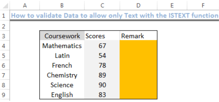 Figure 2: Setting up the Data
Validate Data to Allow Text Only
- We will highlight the range D4:D9 to be validated
- We will go to the Data Tab at the top of the excel sheet
- We will click on “Data Validation,”
- In the Allow field, we will select custom and insert the formula:
=ISTEXT(D4)
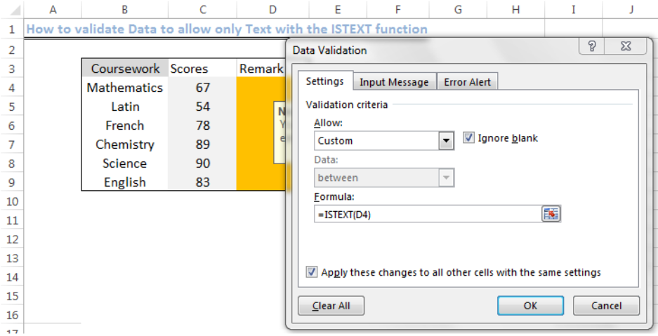 Figure 3: Applying the Data Validation function
- In the Message tab, we will write the error title and error message we wish to see.
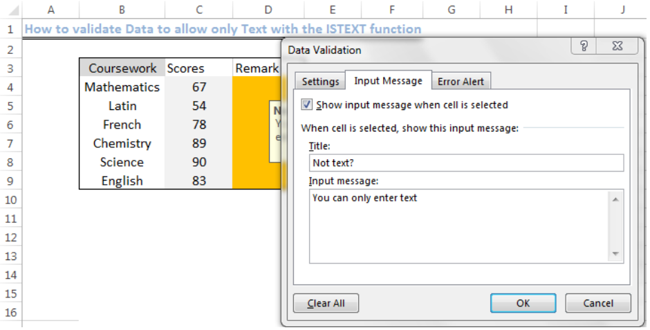 Figure 4: Input the Error text message
- Now, we will click “OK” to apply
- We will click Cell D4 and insert the text we want to see (in this case, “Credit”)
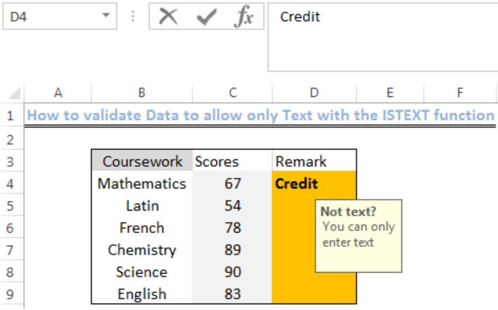 Figure 5: If text, then return TRUE
- In Cell D5, we enter a value, and it returns with the error message.
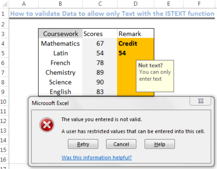 Figure 6: Entered Value is not a Text
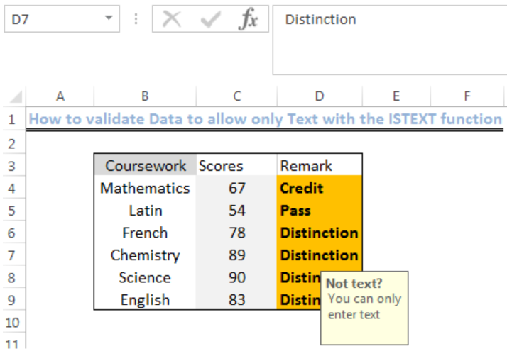 Figure 7: Final Sheet with Text
Explanation
=ISTEXT(D4)
We use the Data validation function and to restrict the kind of data we want in a cell when a user adds or wishes to change the cell value. The ISTEXT function returns TRUE if the value is text and FALSE if not. Because of this, a text will pass the validation, but numbers and formulas will not.
Notes
- We should ensure that the “ignore blank” is clicked
- We can apply the Data validation window minus the input message
- There are many other Data validation functions apart from ISTEXT function
- In the formula field of the data validation window, we can also specify the kind of texts we wish to allow. We should also separate each text with a semicolon or comma depending on the version of Excel we are using.
Instant Connection to an Expert through our Excelchat Service
Most of the time, the problem you will need to solve will be more complex than a simple application of a formula or function. If you want to save hours of research and frustration, try our live Excelchat service! Our Excel Experts are available 24/7 to answer any Excel question you may have. We guarantee a connection within 30 seconds and a customized solution within 20 minutes.
Our Comment Policy.
We welcome your comments and questions about this lesson. We don’t welcome spam. Our readers get a lot of value out of the comments and answers on our lessons and spam hurts that experience. Our spam filter is pretty good at stopping bots from posting spam, and our admins are quick to delete spam that does get through. We know that bots don’t read messages like this, but there are people out there who manually post spam. I repeat — we delete all spam, and if we see repeated posts from a given IP address, we’ll block the IP address. So don’t waste your time, or ours. One other point to note — if you post a link in your comment, it will automatically be deleted.
Add a comment to this lesson
.
Comments on this lesson
Bringing only selected data forward
I have a job costing calculator and i only want to bring text forward to a front sheet in the workbook to summarize the selections. For example: the calculator lists several items offered, I want to bring only the items selected to a front page for a summary of the items selected to that specific job. So if there are 100 items that could be chosen, and only 5 are selected, I want to have a table that shows those 5 items only. AND the items are text not numerical value.
SO the job costing page may have : Window Removal and a cell to populate a number [number of windows to be removed] if that cell has a value greater than 0 i want the text «window removal» brought to another table for summary…I have tried IF functions and am not getting desired result…please help. Thanks
.
Extract number
I would like to extract the number out of column G (Description of goods) into column H (serial numbers) can you assist with a formula
.
Useful tips
Thanks 5 minutes were really 5 minutes and managed to extract data i wanted. Good work.
.
Extracting Numbers From a String
I am trying to separate the numbers from a string of text that contains numbers. The following is a sample string:
C4-14-3-6-21
I’d like to get the numbers into individual cells (except for the C4 part of the string which never changes). 14 is the year and will always be two digits. 3 will eventually become 2 digits long and then 3 and finally 4. The 6 will probably never be more than 2 digits long and the 21 can go 5 or 6 digits long. So far, I was able to create the following formulas that isolated the year (14) and the 3 (next number to the right):
=0+MID(A1,4,FIND(«-«,A1,4)-4)
=0+MID(A1,7,FIND(«-«,A1,7)-7)
It seems to work for the 14 and 3 slots. I haven’t been successful extracting the 6 and 21 (after testing different number of digits). Can you help me get these formulas right to extract all of the numbers?
.
LEFT
In the last exemple «=RIGHT(A1,LEN(A1)-FIND(«.»,A1))» how to do it to get just the names instead of the numbers? Because if you use «=LEFT(A1,LEN(A1)-FIND(«.»,A1))» it give all sting.
Thanks
.
Extract Text from a Cell in Excel
Hi there,
I am trying to extract the set of numbers before the first «~»
My attempt using Formula=RIGHT(A1,LEN(A1)-FIND(«.»,A1)) returned a «0»
3932730~20~17074~S2930248~1~14~S~A-07-02-08~~1
517398~1~17074~S2930248~1~27~S~A-04-07-02
345219~1~17074~S2930248~1~5~S~A-03-01-04
239068~1~17074~S2930248~1~33~S~A-06-05-03
3935400~1~17074~S2930248~1~17~S~A-07-02-03
345219~20~17074~S2930248~1~5~S~A-03-01-04~~1
1742393~1~17074~S2930248~1~36~S~B-16-04-07
Can you please help with this? Kind regards,
Brian
.
Brian,
Brian,
Try using =Left(A1,FIND(«~»,A1)-1)
.
Use Find/Replace
I Know I am very late, but just use replace option with text to find as «~*» and replace with null «»
.
Hello I’m trying to separate
Hello I’m trying to separate specific parts of text from a set of addresses. For example:
800 E DIMOND BLVD STE 127
800 E DIMOND BLVD SUITE 127
320 W 5TH AVE
3048 MOUNTAIN VIEW DR BLDG 119
2120 US HIGHWAY 92 W
On this text I would like to separate the last two parts which are «ste» and «127» to a separate column, the thing is that some addresses don’t have «ste» instead they have «suite» » building», etc. Is there any way that would be possible?
.
Moe,
Moe,
I’m sure it is possible, but I’m not the expert that could tell you how to do it. I’m sorry. I posted my original question to extract a single number from a string of numbers separated by hyphens. Try posting your question as a new string. Good luck.
Regards,
Lubo
.
leaving instead of extracting last octet
I am trying to get only the last octet of an ip address that is in a cell. Instead of using text to columns is there a way to leave only the last octet?
.
no result from Mid command
Col A B C D E F G
Invoice Status Cd State Acct Company Code Invoice Number Invoice Date Contract Number ARN
CO TX S580 65336 1/13/2014 NREC_TX_185584_CTL =MID(F2,9,6)
Using the MID formula listed under the ARN field, I am getting no result whatsoever. Excel 2007 file type .xlxs. What I want is in the ARN column G the number 185584.
.
minor update
dang, it didn’t save my spaces betweent the column numbers. Col F has the Contract Number.
.
extract lot number
6006 — Silicone Tip Capsule Polisher 23gX7mm bend Lot#: 04146016 Loc.: 5
5003AF — Irrigating Cystotome 25gX16mm (5/8″) formed Lot#: 12146050 Loc.: 84-86
Retrobulbar Needle 23gX1 1/2″ (Atkinson Point) Lot#: 01156001
3 different rows, what I need: «Lot#: xxxxxxxx» or just the 5th digit in the lot #, in these rows it would be «6» (if you look at my attachment, Column L & M work for must but since the location [Loc] has a different number of digits, notice cell M3 cuts off some of the Lot #.
TYIA
.
Extracting three different parts of a cell
I need to extract three different parts in the below string of text. I need to extract flavors loved to return «Fruits, Fruits & Cream, Dessert» (it can include quotations in the text. Flavors hated «Tobacco, discovery», then Nicotine level «Low (6mg)
{«flavors_loved»:[«Fruits»,»Fruits & Cream»,»Dessert»],»flavors_hated»:»Tobacco»,»discovery»:»Expand Range»,»nicotine_level»:[«Low (6mg)»]}
.
How to extract numbers within square brackets
Hi,
I have a spreadsheet contains several thousand of records.
These records (column A) contains text strings at and numbers within a square brackets at many various lengths.
What I would like to achieve is how extract just the numbers within the square brackets of column A into a new column. Examples of records as follow;
«Bangalore Street» Beams Road [4069]
«Clifton Hill» O/B Ipswich Road FS Beaudesert Rd [10386]
«HOMEBASE» [3368]
Could someone assist me.
Thanks in advance
.
This is a bit messy, but it
This is a bit messy, but it works.
=mid(A1,find(«[«,A1)+1,find(«]»,A1)-find(«[«,A1)-1)
.
Thanks so much Cionn.
Thanks so much Cionn.
I’ve performed search & replace the open square bracket replaced with symbol then did find formular similar to yours and it works the same way as yours. Thanks for responding to my call for help. Cheers
.
Sorting problem
Below is a sample cell value within my spreadsheet (it’s voting history- general election, primary election). I want to be able to sort using this column. The sorting would be, for example, all persons with a GE14 and a GE12 and a PE11. And various combinations like that. How could I accomplish that?
GE14GE13PE13GE12GE08GE04GE01GE00GE97
.
More information please …
Hi Matt
Can you be more specific about what you want to achieve? You say you want to sort, but I don’t have enough information to decide where, say, someone with GE14, G13 and PE11 might be ranked compared to someone with GE14, GE13 but not PE11.
Also, can you provide a couple of additional samples, and decode the formula? For example, it looks like this is a person who voted in the General Election in 2014, 2013, 2012, 2008, 2004, 2001, 2000 and 1997, and in a Primary Election in 2013. What I can’t tell is whether these are the only years in which elections were held, or if there was, say, a GE every year, but this person didn’t vote in every one of them.
Thanks.
David
.
Hi David. Thanks for the
Hi David. Thanks for the help. The value in this column is that person’s individual voting history. I’m not interested in ranking them. I only want to parcel out those people who, say, voted in GE14, GE12, and GE10. If all three of those values don’t appear in this cell, then (for present sorting purposes) I’m not interested in that person. So I’m wondering what formula I would use. Some sort of if(and(search…As you’ve probably guessed, I’m a novice exceller. Tks for any guidance you can provide.
.
Finding numbers
Hi,
I am a stock markets professional and have an excel file with hundreds of records in the following sample formats:
NIFTY JUN 8500 CE
BANKNIFTY JUL 18800 PE
STAR AUG 1300 CE
INDUSINDBK JAN 900 CE
JPASSOCIAT AUG 10 PE
What I want to do is just extract the numbers out of these cells and use it in a separate formula. I would be grateful if somebody could help me with this.
Regards,
Vikas.
.
Extracting $ amount from a cell
Hello —
Here is an example where all I want to extract is the $4,532.50. I have several like this but not one is the same. I am just looking in that cell for the actual dollar amount and that is it. Is there a formula for that? And it can be in anywhere from $x.xx to $xxx,xxx.xx. Thanks for your assistance.
Archive Hans Wegner Table (DS) AX 2364 $4,532.50 080315 #202061,86 3520
.
Pulling text from the end of a string to a new column
Pulling text from the end of a string to a new column, with different length prefixes. I really need some help here 
I need to get the size indicator of the end of the Sku into the next column
The M, XL, L and S
How can I do this because they are different lengths?
.
This formula is almost what I need to do.
Hello,
This formula is what I need, but I need to see another step. In my case I do have » : » and I need to grab everything as the last » : «
Example:
MY Part number: Susp IP:Torsion bars:911:1-SAW911F19
I need to grab the last part of the number just this part 1-SAW911F19
This formula almost gets me what I need =RIGHT(A1,LEN(A1)-FIND(«:»,A1)) but it get me everything after the first » : «
Thank you for your help.
VH
.
Very percise and satisfying
Very percise and satisfying answer. Thank you so much, you are very helpful.
.
Same Problem here
Did you solve your problem? Mine is very similar.
rumo-log-RUMO3
bmfbovespa-BVMF3
vale-VALE5
itausa-ITSA4
banco-do-brasil-BBAS3
itau-unibanco-ITUB4
guarapes-GUAR4
braskem-BRKM5
estacio-participacoes-ESTC3
br-malls-par-BRML3
brasilagro-AGRO3
cosan-ltd-CZLT33
unicasa-UCAS3
grendene-GRND3
alupar-ALUP11
fii-cshg-jhsf-HGJH11
fii-bc-fund-BRCR11
portobello-PTBL3
mills-MILS3
cielo-CIEL3
I’m trying to get only the last caps words. This formula =RIGHT(B3;LEN(B3)-FIND(«-«;B3)) works great with data with only 2 words, but the rest bring me stuff that I dont need
.
Found it
This worked for me! =TRIM(RIGHT(SUBSTITUTE(E2,»-«,REPT(» «,100)),100))
Hope it works for you too!
.
pulling text of different lengths
I am trying to pull the model of a product (text and numerical) from the beginning of each cell into another column for total product model analysis. Some models have one word, some have 3-4 words plus a number.
example:
Big River P 700c, 555, 0
Spy Hill 7.3 P 27.5, L3, 0
Glass Creek Pro Carbon Q, 29, 0
I would like to extract:
Big River
Spy Hill 7.3
Glass Creek Pro Carbon
See attached for actual data
.
Extracting
ip address 10.10.10.10
ip address 10.10.10.11
ip address 10.10.10.12
.
.
How can we extract only: 10.10.10.10 and 10.10.10.11 and so on?
.
string with unequal characters with 2 delimiters
My data is of different lengths, and the only constant is that the part I want to remove is always the last 11 characters. Alternatively, the data I want to retrieve is up to but not including the second underscore: Here is a sample:
R5510BU010_MAIN_926030_PDF
R5510BU010_MAIN_926028_PDF
R5510BU021_ALL_925732_PDF
R5510BU021_REGULAR_926026_PDF
R5510BU010_MAIN_925736_PDF
R5510BU021_REGULAR_925734_PDF
R5510BU010_MAIN_925738_PDF
R5510BU021_ALL_926024_PDF
R5510BU021_REGULAR_925468_PDF
R5510BU010_MAIN_925470_PDF
R5510BU010_MAIN_925472_PDF
What I am trying to do is retrieve everything up to but not including the second underscore. I can’t use left because the fields are unequal lengths, and when I use right, it returns the stuff I’m trying to remove.
Is there a better way?
Thanks
.
Addendum to above question
Sorry, I forgot to add:
I tried this formula: =LEFT(G2,LEN(G2)-FIND(«_»,G2)) and it returned:
R5510BU010_MAIN
R5510BU010_MAIN
R5510BU021_ALL
R5510BU021_REGULAR
R5510BU010_MAIN
R5510BU021_REGULAR
R5510BU010_MAIN
R5510BU021_ALL
R5510BU021_REGULAR
R5510BU010_MAIN
R5510BU010_MAIN
This looks great, but when I copied to down to the rest of the cells I got this:
R09801_ZJDE0002_926264_PDF returned R09801_ZJDE0002_926
R09801_ZJDE0002_925803_PDF returned R09801_ZJDE0002_925
R09801_ZJDE0002_925801_PDF returned R09801_ZJDE0002_925
R09801_ZJDE0002_925805_PDF returned R09801_ZJDE0002_925
R09801_ZJDE0002_925807_PDF returned R09801_ZJDE0002_925
R09801_ZJDE0002_925809_PDF returned R09801_ZJDE0002_925
R09801_ZJDE0002_925811_PDF returned R09801_ZJDE0002_925
R09801_ZJDE0002_926290_PDF returned R09801_ZJDE0002_926
Why did it seem to understand in the first selection but not the second?
Thanks
.
Ease of access to specific issues in 5 minute lessons
Thank you very much for putting up 5 minute lessons. They work better than excel help menu and the explanations are far more comprehensive & useful. I use 5 minute lesson as my excel help menu.
.
Extract text from a cell
I have a situation where I need to extract some or all of the DATA in a cell.
I am an options trader and at the end of the day i would like to know the underlying stock symbol for the option which will help easily filter and sort the trades.
stock symbols normally range between 1 and 4 letters
GDX
GDX 160708P28
GDX 160708P28
BBRY 160916C9
SLV 160805C19.5
SLV
=LEFT(B11,FIND(» «,B11))
This works fine for the option chain, but if its just the stock»SLV» it returns an error
The values im looking for are listed below
GDX
GDX
GDX
BBRY
SLV
SLV
Thanks for your help
.
Extracting Multiple info from a string of text
The below contains info found in a cell separated by commas. I’d to separate each of the info grouped by commas and put into different cells. At the moment I can only extract only the first set «PKL70080P» using =LEFT(A65,FIND(«,»,A65)-1). The rest I’m not sure how to do that.
PKL70080P,»Tbitha 318* x .02 LB OPT»,TPLin,5/12/2011,19,81,96,82,91,81,85,98,94,95,92,98,80,N/A,»»
Thanks!
.
Extracting ‘Sub ID’
I am trying to extract a 32 alphanumeric subscription ID out of the Forecast Comments column. Forecast comments are essentially notes exported from our CRM system. The majority of the sales reps have «Sub ID[space]» prior to the IS, so I tried =RIGHT(J2,LEN(J2)-FIND(«Sub ID «,J2)) but I got an error. Also I don’t want all the notes that are in the cell AFTER the Sub ID.
.
i was lost in hope and faith
i was lost in hope and faith when i was unable to get into my account that i save all my document and file ,but thanks to cyberhelp company who help me get into my account and get everything back for me with no stress just give them some info and everything is done within 5hours really amazing to work with them ,thats why im so proud to recommend they to people to use them and they will never disappoint you ,,contact them on ( cyberhelp027 @ …gmail .com ) and you thanks me later
or text them on +160 64413481 or What Sapp +1 7863616429
.
Extracting Data from one cell to copy in another
Hi,
I am trying to find a way of extracting only part of a cells contents if it contains certain characteristics. So in cell C2 I have a long bank narrative which may contain a policy number. They number always begin with the same 2 letters for example AB followed by 7 numbers.
How can I get excel to check C2 and if it contains anything which begins AB followed by 7 numbers it will copy the policy number to cell G2? The policy number could be anywhere in the text so it needs to be able to go through the whole cell content.
Thanks for any help you can give
.
.
.
.
Sometimes you may have the text and numeric data in the same cell, and you may have a need to separate the text portion and the number portion in different cells.
While there is no inbuilt method to do this specifically, there are some Excel features and formulas you can use to get this done.
In this tutorial, I will show you 4 simple and easy ways to separate text and numbers in Excel.
Let’s get to it!
Separate Text and Numbers Using Flash Fill
Below I have the employee data in column A, where the first few alphabets indicate the department of the employee and the numbers after it indicates the employee number.

From this data, I want to separate the text part and the number part and get these into two separate columns (columns B and C).
The first method that I want to show you to separate text and numbers in Excel is by using Flash Fill.
Flash Fill (introduced in Excel 2013) works by identifying patterns based on user input.
So if I manually enter the expected result in column B, Flash Fill will try and decipher the pattern and give me the result for all the cells in that column.
Below are the steps to separate the text part from the cell and get it in column B:
- Select cell B2
- Manually enter the expected result in cell B2, which would be MKT

- With cell B2 selected, place the cursor at the bottom right part of the selection. You’ll notice that the cursor changes into a plus icon (this is called Fill Handle)

- Hold the left mouse/trackpad key and drag the Fill Handle to fill the cells. Don’t worry if the cells are filled with the same text
- Click on the Auto Fill Options icon and then select the ‘Flash Fill’ option

The above steps would extract the text part from the cells in column A and give you the result in column B.

Note that in some cases, Flash Fill may not be able to identify the right pattern. In such cases, it would be best to enter the expected result in two or three cells, use the Fill Handle to fill the entire column, and then use Flash Fill on this data.
You can follow the same process to extract the numbers in column C. All you need to do is enter the expected result in cell C2 (step 2 in the process laid out above)
Note that the result you get from Flash Fill is static and would not update in case you change the original data in column A. If you want the result to be dynamic, you can use the formula method covered next.
Separate Text and Numbers Using Formula
Below I have the employee data in column A and I want to use a formula to extract only the text part and put it in column B and extract the number part and put it in column C.
Since the data is not consistent (i.e., the alphabets in the department code and the numbers in the employee number are not of the consistent length), I cannot use the LEFT or RIGHT function to extract only the text portion or only the number portion.
Below is the formula that will extract only the text portion from the left:
=LEFT(A2,MIN(IFERROR(FIND({0,1,2,3,4,5,6,7,8,9},A2),""))-1)

And below is the formula that will extract all the numbers from the right:
=MID(A2,MIN(IFERROR(FIND({0,1,2,3,4,5,6,7,8,9},A2),"")),100)

How does this formula work?
Let me first explain the formula that we use to separate the text part on the left.
=LEFT(A2,MIN(IFERROR(FIND({0,1,2,3,4,5,6,7,8,9},A2),””))-1)
The FIND part in the formula finds the position of digits 0 to 9 in cell A2. In case it finds that digit in cell A2, it returns the position of that digit, and in case it is not able to find that digit, then it returns the value error (#VALUE!)
For cell A2, it gives a result as shown below:
{#VALUE!,4,#VALUE!,#VALUE!,#VALUE!,6,#VALUE!,5,#VALUE!,#VALUE!}
- For 0, it returns #VALUE! as it cannot find this digit in cell A2
- For 1, it returns 4 as that is the position of the first occurrence of 1 in cell A2
- and so on…
This FIND formula is then wrapped inside the IFERROR function, which removes all the value errors but leaves the numbers.
The result of it looks like as shown below:
{“”,4,””,””,””,6,””,5,””,””}
The MIN function then goes through the above result and gives us the minimum value from the results. Since each number in the array represents the position of that corresponding number, the minimum value tells us where the numerical value starts in the cell.
Now that we know where the numerical values start, I have used the LEFT function to extract everything before this position (which would be all the text in the cell).
Similarly, you can use the same formula with a minor tweak to extract all the numbers after the text. To extract the numbers, where we know the starting position of the first digit, use the MID function to extract everything starting from that position.
And what if the situation is reversed – where we have the numbers first and the text later and we want to separate the numbers and text?
You can still use the same logic with one minor change – instead of finding the minimum value that gives us the position of the 1st digit in the cell, you need to use the MAX function To find the position of the last digit in this cell. Once you have it, you can again use the LEFT function or the MID function to separate the numbers and text.
Separate Text and Numbers Using VBA (Custom Function)
While you can use the formulas shown above to separate the text and numbers in a cell and extract these into different cells – if this is something you need to do quite often, you also have the option to create your own custom function using VBA.
The benefit of creating your own function would be that it would be a lot easier to use (with just one function that takes only one argument).
You can also save this custom function VBA code into the Personal Macro Workbook so that it would be available in all your Excel workbooks.
Below the VBA code that could create a function ‘GetNumber’ that would take the cell reference as the input argument, extract all the numbers in the cell, and give it as the result.
'Code created by Sumit Bansal from https://trumpexcel.com
'This code will create a function that can separate numbers from a cell
Function GetNumber(CellRef As String)
Dim StringLength As Integer
StringLength = Len(CellRef)
For i = 1 To StringLength
If IsNumeric(Mid(CellRef, i, 1)) Then Result = Result & Mid(CellRef, i, 1)
Next i
GetNumber = Result
End Function
And below the VBA code that would create another function ‘GetText’ that would take the cell reference as the input argument and give you all the text from that cell
'Code created by Sumit Bansal from https://trumpexcel.com
''This code will create a function that can separate text from a cell
Function GetText(CellRef As String)
Dim StringLength As Integer
StringLength = Len(CellRef)
For i = 1 To StringLength
If Not (IsNumeric(Mid(CellRef, i, 1))) Then Result = Result & Mid(CellRef, i, 1)
Next i
GetText = Result
End Function
Below are the steps to add this code to your excel workbook so that this function becomes available for you to use in the worksheet:
- Click the Developer tab in the ribbon
- Click on the Visual Basic icon

- In the Visual Basic editor that opens up, you would see the Project Explorer on the left. This would have the workbook and the worksheet names of your current Excel workbook. If you don’t see this, click on the View option in the menu and then click on Project Explorer

- Select any of the sheet names (or any object) for the workbook in which you want to add this function
- Click on the Insert option in the top toolbar and then click on Module. This will insert a new module for that workbook

- Double click on the module icon in ‘Project Explorer’. This will open the module code window.

- Copy and paste the above custom function code into the module code window

- Close the VB Editor
With the above steps, we have added the custom function code to the Excel workbook.
Now you can use the functions =GETNUMBER or =GETTEXT just like any other worksheet function.
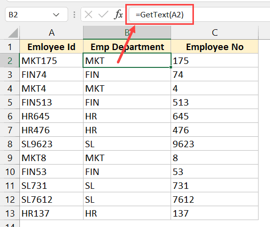
Note – Once you have the macro code in the module code window, you need to save the file as a Macro Enabled file (with the .xlsm extension instead of the .xlsx extension)
If you often have a need to separate text numbers from cells in Excel, it would be more efficient if you copy these VBA codes for creating these custom functions, and save these in your Personal Macro Workbook.
You can learn how to create and use Personal Macro Workbook in this tutorial I created earlier.
Once you have these functions in the Personal Macro Workbook, you would be able to use these on any Excel workbook on your system.
One important thing to remember when using functions that are stored in Personal Macro Workbook – you need to prefix the function name with =PERSONAL.XLSB!. For example, if I want to use the function GETNUMBER in a workbook in Excel, and I have saved the code for it in the postal macro workbook, I will have to use =PERSONAL.XLSB!GETNUMBER(A2)
Separate Text and Numbers Using Power Query
Power Query is slowly becoming my favorite feature in Excel.
If you’re already using Power Query as a part of your workflow, and you have a data set where you want to separate the text and numbers into separate columns, Power Query will do it in a few clicks.
When you have your data in Excel and you want to use Power Query to transform that data, one prerequisite is to convert that data into an Excel Table (or a named range).
Below I have an Excel Table that contains the data where I want to separate the text and number portions into separate columns.

Here are the steps to do this:
- Select any cell in the Excel Table
- Click the Data tab in the ribbon

- In the Get and Transform group, click on the ‘From Table/Range’

- In the Power Query editor that opens up, select the column from which you want to separate the numbers and text
- Click the Transform tab in the Power Query ribbon

- Click on the Split Column option

- Click on ‘By Non Digit to Digit’ option.

- You’ll see that the column has been split into two columns where one has only the text and the other only has the numbers

- [Optional] Change the column names if you want
- Click the Home tab and then click on Close and Load. This will insert a new sheet and give us the output as an Excel Table.

The above steps would take the data from the Excel Table we originally had, use Power Query to split the column and separate the text and the number parts into two separate columns, and then give us back the output in a new sheet in the same workbook.

Note that we used the option ‘By Non-Digit to Digit’ option in step 7, which means that every time there is a change from a non-digit character to a digit, a split would be made. If you have a dataset where the numbers are first followed by text, you can use the ‘By Digit to Non-Digit’ option
Now let me tell you the best part about this method. Your original Excel Table (which is the data source) is connected to the output Excel Table.
So if you make any changes in your original data, you don’t need to repeat the entire process. You can simply go to any cell in the output Excel Table, right click and then click on Refresh.
Power query would run in the back end, check the entire original data source, do all the transformations that we did in the steps above, and update your output result data.
This is where Power Query really shines. If there is a set of transformations that you often need to do on a data set, you can use Power Query to do that transformation once and set the process. Excel would create a connection between the original data source and the resulting output data and remember all the steps you had taken to transform this data.
Now, if you get a new data set you can simply put it in the place of your original data and refresh the query, and you will get the result in a few seconds. Alternatively, you can simply change the source in Power Query from the existing Excel table to some other Excel Table (in same or different workbook).
So these are four simple ways you can use to separate numbers and text in Excel. if this is a once-in-a-while activity, you’re better off using Flash Fill or the formula method.
And in case this is something you need to do quite often, then I would suggest you consider the VBA method where we created a custom function or the Power Query method.
I hope you found this Excel tutorial useful.
Other Excel tutorials you may also like:
- Separate First and Last Name in Excel (Split Names Using Formulas)
- How to Convert Numbers to Text in Excel
- Convert Text to Numbers in Excel – A Step By Step Tutorial
- How to Compare Text in Excel
- How to Quickly Combine Cells in Excel
- How to Combine First and Last Name in Excel
- How to Extract the First Word from a Text String in Excel (3 Easy Ways)
- Extract Numbers from a String in Excel (Using Formulas or VBA)
- How to Extract a Substring in Excel (Using TEXT Formulas)
Microsoft Excel is a great tool, but sometimes the spreadsheet files we get to work with aren’t ideal. One example is a file with a data column, maybe a street address, that you’d really like to pull apart. In this tutorial, I’ll show how to extract text from a cell in Excel using some powerful, but simple text functions. (Includes practice workbook.)
What’s an Excel Substring?
Before we have Excel extract text from string, we need to define some things. Some programming languages have dedicated substring functions. Excel does something similar using Text functions. They have their own category.

When we speak of a substring, we mean a part or subset of the Excel cell’s content. For example, if the cell contained 1001 Drake Ave., any of these items could be a substring:
- 1001
- Drake Ave.
- 100
- rake
A Common Problem
Many membership databases or mailing lists are set up with defined fields for First Name, Last Name, Street, City, State, and Zip. This format works fine if you’re creating a mailing label as the post office relies on zip code sorting. And sometimes you can luck out and parse first and last names using Excel’s Convert Text to Columns Wizard.
But what if you need to do door-to-door canvassing to check on neighbors or to inform people about an upcoming ballot measure?
If you open this type of list in Excel and sort it on the Street column, you get a numerically sorted list. As you can see in the example below, the Drake Ave records are not together.
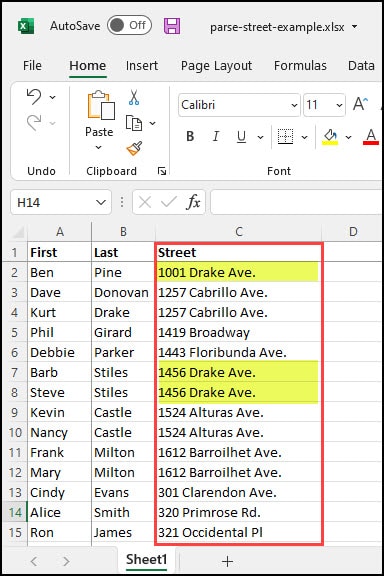
Ideally, you want to sort the list so the Drake Ave. entries are together. There are several ways to do this in Excel, but one way is to create two columns from the Street column.
The first column reflects the street number substring, and the second the street name substring. You can then resort the list based on the street name and street number.
Visually Building the Nested Formula
For the first example, we’ll nest some Excel functions such as LEFT and FIND. As we progress, we’ll add several sets of parentheses. By nested, I mean we’ll use one function (FIND) as an argument for another function such as LEFT or RIGHT.
Let’s start with =FIND(" ",C2). In plain text, our function syntax is asking Excel to look in reference cell C2 for a blank space which is represented by the ” “. In the picture below, I added a starting position of “1“, but this is an optional parameter and Excel starts at 1 by default. Excel found the blank space in position 5 which shows in cell D2.

To make the formula easier, I’ll remove the optional starting parameter of 1 since Excel starts there anyway.
Now, let’s add the LEFT function so that our formula reads =LEFT(C2,(FIND(" ",C2))). In this instance, we’re again using cell C2, but the LEFT function is going to grab the cell contents in C2 from position 1 to position 5 where the Excel FIND function found the blank space.

However, there is a minor issue. While you can’t see it, there is a trailing space in D2. Using the LEN function we can see cell D2 has 5 characters. You may remember this handy function from our tutorial on how to check character count in Excel.

The solution is to subtract 1 or use the TRIM function which I referenced in how to separate names in Excel. For simplicity, I’ll use the -1. While the visual results are the same, you can see the character count dropped by 1.

- Import your data into Microsoft Excel or use the sample spreadsheet in the Resources section.
- In cell D1, type Nbr.
- In cell E1, type Street Name
- In cell D2, type the following Excel formula
=LEFT(C2,(FIND(" ",C2)-1)) - Press Enter. The value 1001 should show in D2.
The next part involves copying this formula to the rest of the entries. However, we need to reference the correct street cell and not use C2 for the remaining rows.
- Click cell D2 to select the beginning of our range.
- Move your mouse to the lower right corner.

- Double-click the + cursor in the lower right. This will copy your formula down the column.
In column D, you should see the extracted street numbers.
We’ll now create a similar nested formula to capture the street address using the RIGHT function. This time, we will grab the contents to the right of the first space from the Street column.
- In cell E2, type the following formula
=RIGHT(C2,LEN(C2)-FIND(" ",C2)) - Press Enter. E2 should show as Drake Ave.
- Click cell E2 to select the beginning of our range.
- Move your mouse to the lower right corner.
- Double-click the + cursor in the lower right. This will copy your formula down the column.
Columns D and E should contain the parsed contents from your original street address.
Your spreadsheet should look similar to the one below.

Clean Up the Spreadsheet and Change Cell Format
The spreadsheet now has your split fields, but you should clean up the formulas. My suggestion would be to convert the LEFT and RIGHT formulas to their respective values. We did an earlier tutorial on how to copy formula values in Excel to values.
After you convert the Nbr column, you probably want to change the format type to a number.
- Click column D.
- Right-click and select Format cells...
- On the Format Cells dialog box, select Number.
- Set Decimal places to 0.
- Click OK.
Although our example extracted text from an Excel cell containing street information, you can use the same process to parse other entries. For example, Step 1 above is really parsing everything but the first word because it is searching for a blank space. You can alter the formula to find different values, such as a comma or an @ sign.
Excel Practice File
Hand-picked Excel Tutorials
-
10-29-2012, 08:43 AM
#1

Registered User
how to show only text in excel cell?
in my excel column shows number and text, i want to hide number, has to shows only text. i have attached my excel sheet as well. In Relationship and Entity common name. the data inside these columns are «number;#and then value like «Client» or «Vendor»(2;#Vendor). so what i wanted to do is, need to display only «Vendor». how can i do it? i have to apply the formulas for whole «D» and «E». Please guide me.
-
10-29-2012, 02:42 PM
#2
Forum Contributor
Re: how to show only text in excel cell?
Try this in a new column. I inserted one between E and F of your example sheet.
-
10-30-2012, 06:14 AM
#3
Registered User
Re: how to show only text in excel cell?
Excellent, it works fine. Thanks a lot

