
Excel for Microsoft 365 Excel for the web Excel 2021 Excel 2019 Excel 2016 Excel 2013 Excel 2010 Excel 2007 More…Less
Microsoft Excel can wrap text so it appears on multiple lines in a cell. You can format the cell so the text wraps automatically, or enter a manual line break.
Wrap text automatically
-
In a worksheet, select the cells that you want to format.
-
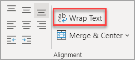
On the Home tab, in the Alignment group, click Wrap Text. (On Excel for desktop, you can also select the cell, and then press Alt + H + W.)

Notes:
-
Data in the cell wraps to fit the column width, so if you change the column width, data wrapping adjusts automatically.
-
If all wrapped text is not visible, it may be because the row is set to a specific height or that the text is in a range of cells that has been merged.
-
Adjust the row height to make all wrapped text visible
-
Select the cell or range for which you want to adjust the row height.
-
On the Home tab, in the Cells group, click Format.
-
Under Cell Size, do one of the following:
-
To automatically adjust the row height, click AutoFit Row Height.
-
To specify a row height, click Row Height, and then type the row height that you want in the Row height box.
Tip: You can also drag the bottom border of the row to the height that shows all wrapped text.
-
Enter a line break
To start a new line of text at any specific point in a cell:
-
Double-click the cell in which you want to enter a line break.
Tip: You can also select the cell, and then press F2.
-
In the cell, click the location where you want to break the line, and press Alt + Enter.
Need more help?
You can always ask an expert in the Excel Tech Community or get support in the Answers community.
Need more help?
Want more options?
Explore subscription benefits, browse training courses, learn how to secure your device, and more.
Communities help you ask and answer questions, give feedback, and hear from experts with rich knowledge.
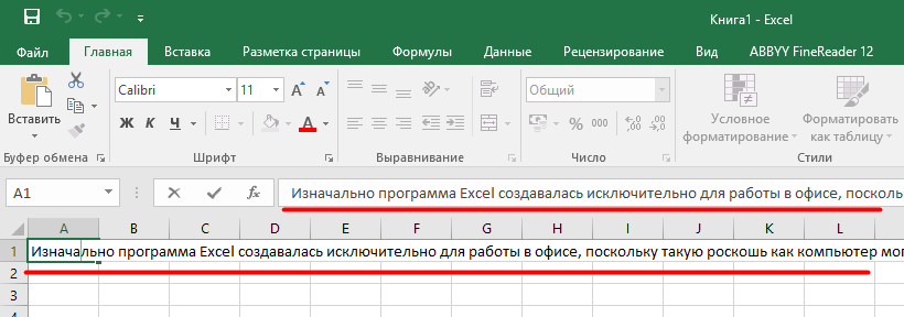
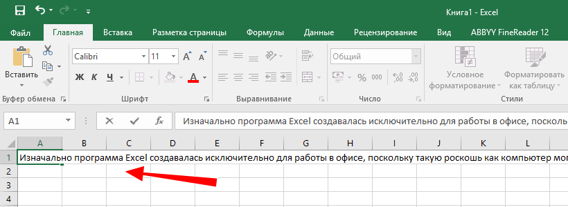
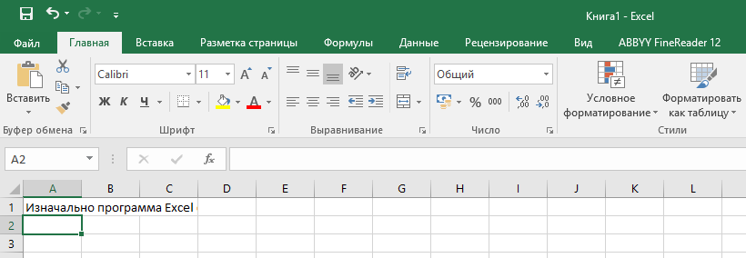
When you enter a text string in Excel which exceeds the width of the cell, you can see the text overflowing to the adjacent cell(s).
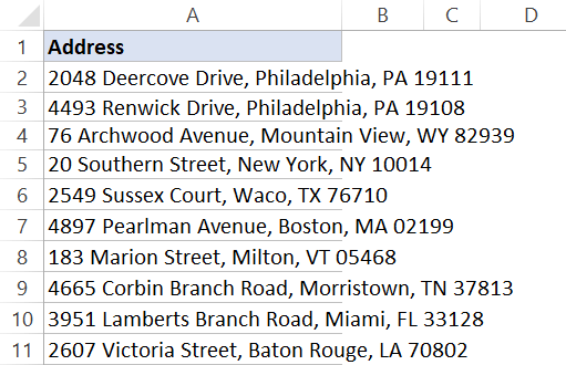
Below is an example where I have some address in column A and these address overflow to the adjacent cells as well.
And in case you have some text in the adjacent cell, the otherwise overflowing text would disappear and you will only see the text that can fit the cell column width.
In both cases, it doesn’t look good and you may want to wrap the text so that the text remains within a cell and not spill over to others.
This can be done using the wrap text feature in Excel.
In this tutorial, I will show you various ways of wrapping text in Excel (including doing it automatically with a single click, using a formula and doing it manually)
So let’s get started!
Wrap text with a Click
Since this is something you may need to do quite often, there is easy access to quickly wrap the text with a click on a button.
Suppose you have the dataset as shown below where you want to wrap text in column A.
Below are the steps to do this:
- Select the entire dataset (column A in this example)
- Click the Home Tab

- In the Alignment group, click on the ‘Wrap text’ button.


That’s It!
All it takes it two-click to quickly wrap the text.
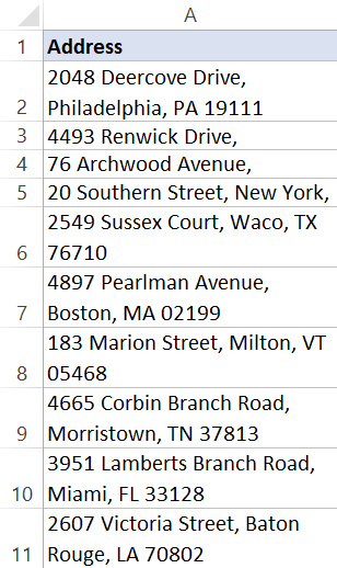
You will get the final result as shown below.
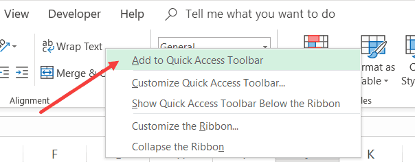
You can further bring down the effort from two to one-click by adding the Wrap text option to the Quick Access Toolbar. To do this. right-click on the Wrap text option and click on ‘Add to Quick Access Toolbar’
This adds an icon to the QAT and when you want to wrap text in any cell, just select it and click this icon in the QAT.
Wrap text with a Keyboard Shortcut
If you’re like me, leaving the keyboard and using a mouse to click even a single button could feel like a waste of time.
Good news is that you can use the below keyboard shortcut to quickly wrap text in all the selected cells.
ALT + H + W (ALY key followed by the H and W keys)
Wrap text with the Format Dialog box
This is my least preferred method, but there is a reason I am including this one in this tutorial (as it can be useful in one specific scenario).
Below are the steps to wrap the text using the Format dialog box:
- Select the cells for which you want to apply the wrap text formatting
- Click the Home tab
- In the Alignment group, click on the Alignment Setting dialog box launcher (it’s a small ’tilted arrow in a box’ icon at the bottom right of the group).

- In the ‘Format Cells’ dialog box that opens, select ‘Alignment’ tab (if not selected already)
- Select the Wrap text option

- Click OK.


The above steps would wrap the text in the selected cells.
Now if you’re thinking why to use this twisted long method when you can use a keyboard shortcut or a single click on the ‘Wrap Text’ button in the ribbon.
In most cases, you should not be using this method, but it can be useful when you want to change a couple of formatting settings. Since the Format Dialog box gives you access to all the formatting options, this may end up saving you some time.
NOTE: You can also use the keyboard shortcut Control + 1 to open the ‘Format Cells’ dialog box.
How Does Excel Decide How Much text to Wrap
When you use the above method, Excel uses the column width to decide how many lines you get after wrapping.
Doing this makes sure that anything that you have in the cell is confined within the cell itself and doesn’t overflow.
In case you change the column width, the text will also adjust to ensure it fits the column width automatically.
Inserting Line Break (Manually, Using Formula, or Find and Replace)
When you apply ‘Wrap Text’ to any cell, Excel determines the line breaks based on the width of the column.
So if there is text which can fit in the existing column width, it will not be wrapped, but in case it can not, Excel will insert the line breaks by first fitting the content in the first line and then moving the rest to the second line (and so on).
By entering a line break manually, you force Excel to move the text to the next line (in the same cell) right after the line break is inserted.
To enter the line break manually, follow the below steps:
- Double-click on the cell in which you want to insert the line break (or press F2). This will get you into the edit mode in the cell
- Place the cursor where you want the line break.
- Use the keyboard shortcut – ALT + ENTER (hold the ALT key and then press Enter).
Note: For this to work, you need to have Wrap Text enabled on the cell. If Wrap Text is not enabled, you will see all the text in one single line, even if you have inserted the line break.
You can also use a CHAR formula to insert a line break (as well as a cool Find and Replace trick to replace any character with a line break).
Both of these methods are covered in this short tutorial on inserting line breaks in Excel.
And in case you want to remove line breaks from cells in Excel, here is a detailed tutorial about it.
Handling Wrapping Too Much Text
Sometimes you may have a lot of text in a cell and when you wrap the text, it may end up making your row height large.
Something as shown below (the text is taken for bookbrowse.com):
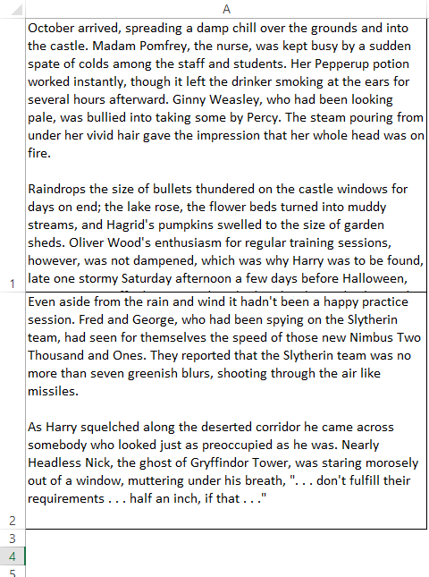
In such a case, you may want to adjust the row height and make it consistent. The downside of this is that not all the text in the cell will be visible, but it makes your worksheet a lot more usable.
Below are the steps to set the row height of the cells:
- Select the cells for which you want to change the row height
- Click the ‘Home’ tab
- In the Cells group, click on the ‘Format’ option

- Click on Row Height

- In the ‘Row Height’ dialog box, enter the value. I am using the value 40 in this example.

- Click OK


The above steps would change the row height and make it all consistent. In case any of the selected cells have text which can not be fit in a cell with the specified height, it will be cut from the bottom.
Don’t worry, the text would still be in the cell. It just won’t be visible.
Excel Text Wrap Not Working – Possible Solutions
In case you find that the Wrap text option is not working as expected and you still see the text as a single line in the cell (or with some missing text), there could be a few possible reasons:
Wrap Text is not enabled
Since it works as a toggle, quickly check whether it’s enabled or not.
If it’s enabled, you will see that this option is highlighted in the Home tab
Cell height needs to be adjusted
When Wrap Text is applied, it moves the extra lines below the first line in the cell. In case your cell row height is less, you may not see the entire wrapped text.
In that case, you need to adjust the cell height.
You change the row height manually by dragging the bottom edge of the row.
Alternatively, you can use the ‘AutoFit Row Height’. This option is available in the ‘Home’ tab in ‘Format’ options.
To use the AutoFit option, select all the cells that you want to auto-fit and click on the AutoFit Row Height option.
The Column Width is Already Wide enough
And sometimes there is nothing wrong.
When your column width is wide enough, there is no reason for Excel to wrap the text as it already fits the cell in a single line.
In case you still want the text to split into multiple lines (despite having enough column width), you need to insert the line break manually.
Hope you found this tutorial useful.
You may also like the following Excel tutorials:
- How to Find Merged Cells in Excel
- How to Merge Cells in Excel
- Excel Text to Columns
- Insert Bullet Points in Excel
- How to Insert a Check Mark (Tick Mark) Symbol in Excel
A normal Excel sheet has cells that are 8.43 points in width and 15 points in height. This is usually about 64 pixels wide and 20 pixels tall.
If your text data is long, you can increase the cell width to fit the data length.
A better option might be to wrap the text to increase the row height so the data fits in the cell instead!
In this post you’ll learn 3 ways to wrap your text data to fit it inside the cell.
What is Text Wrap?
This means that if text is too long to fit inside its cell, it will automatically adjust to appear on multiple lines within the cell.
The data inside the cell will not change and no line break characters will be inserted. It will only appear to be formatted on multiple lines.
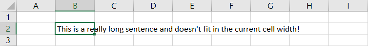
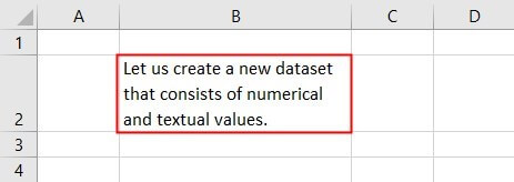
The above example you can see the text inside cell B2 extends well past the width of the cell and spills over cell to the right.
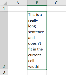
After the cell has had wrap text applied, you can see the row height has been adjusted to fit all the text.
Wrap Text from Ribbon
This is a very common action, so it can be found in the Home tab of the ribbon commands.
Wrap your text.
- Select the cell or range of cells to which you want to apply the wrap text formatting.
- Go to the Home tab.
- Press the Wrap Text command found in the Alignment section.
This will apply the formatting to your cells!
It’s a good idea to adjust the width of your cells to the desired size first as the height of the rows will be adjusted so all the text fits inside the cell.
Wrap Text Keyboard Shortcut
There is no dedicated keyboard shortcut for the wrap text formatting, but you can still use the Alt hotkeys for this.
Select the cells to which you want to apply wrap text then press Alt ➜ H ➜ W.
Certainly a quick and easy way to apply the formatting.
Wrap Text in the Format Cells Dialog Box
The format cells dialog box contains all the formatting options you can apply to a cell in your spreadsheet, including the wrap text option.
You can open this menu with a right click on the cells then choose Format Cells or by using the Ctrl + 1 keyboard shortcut.
Go to the Alignment tab in the menu ➜ Check the Wrap text option in the Text control section ➜ then press the OK button.
This is a great option when you want to apply wrap text and other formatting options at the same time.
Automatically Adjust Row Height to Fit Text
If your row height does not properly adjust to fit all the text and is either too small or too big, then you will need to adjust it.
You can do this manually by clicking and dragging the row but there is an easy option to auto-adjust the height.
Go to the Home tab ➜ select the Format options ➜ then select AutoFit Row Height from the menu. You can also do this by double clicking on the edge of the row heading.
The row height will adjust to the exact height needed to show all the text.
Manually Add Line Breaks to Wrap Your Text
The wrap text option will automatically format your text with line breaks based on the available width of the cell.
If you want to choose where the line breaks appear, then you can do this by manually adding line break characters to your text data.
Place the cursor in the text at the point where you want to add a line break then hold the Alt key and press Enter.
This will add a line break character into your text data and the data will appear on multiple lines in the sheet.
Remove Wrap Text
It’s just as easy to remove wrap text formatting as it is to apply it in the first place.
Remove Formatting
Select the cells from which you want to remove the formatting and then perform any of these methods.
- Go to the Home tab and press the Wrap Text command.
- Open the Format Cells menu and uncheck the Wrap text option in the Alignment tab.
- Use the Alt ➜ H ➜ W keyboard shortcut.
The exact same commands used to apply the formatting can be used to remove the formatting as well!
Remove Manually Added Line Breaks
If you’ve manually added line break characters to your text to achieve a wrapping effect, then you will need to remove them using a find and replace method.
Press Ctrl + H to open the find and replace dialog box.
Place the cursor in the Find what section and press Ctrl + J to add a line break character. Leave the Replace with section empty and then press the Replace All button.
This will replace all the line break character that you manually added by nothing thereby removing them.
Conclusions
Wrapping text is a great option for styling your spreadsheets and making them more readable.
It’s great too, because it’s very easy to do.
What’s your favourite method? Let me know in the comments!
About the Author
John is a Microsoft MVP and qualified actuary with over 15 years of experience. He has worked in a variety of industries, including insurance, ad tech, and most recently Power Platform consulting. He is a keen problem solver and has a passion for using technology to make businesses more efficient.
Содержание
- Wrap text in a cell
- Wrap text automatically
- Adjust the row height to make all wrapped text visible
- Enter a line break
- Need more help?
- Wrap text in a cell
- Wrap text automatically
- Adjust the row height to make all wrapped text visible
- Enter a line break
- Need more help?
- Перенос текста в ячейке Excel
- Перенос текста в одной ячейке Excel
- Перенос текста в объединенных ячейках Excel
- Как сделать перенос строки в ячейке Excel
- С помощью «горячих клавиш»
- Перенос строки в ячейке Excel формулой
- Как скрыть длинный текст в ячейке Excel
- How to wrap text in Excel
- What is wrap text in Excel?
- How to wrap text in Excel automatically
- How to unwrap text in Excel
- How to insert a line break manually
- Excel wrap text not working
- 1. Fixed row height
- 2. Merged cells
- 3. The cell is wide enough to display its value
- 4. Horizontal alignment is set to Fill
Wrap text in a cell
Microsoft Excel can wrap text so it appears on multiple lines in a cell. You can format the cell so the text wraps automatically, or enter a manual line break.
Wrap text automatically
In a worksheet, select the cells that you want to format.
On the Home tab, in the Alignment group, click Wrap Text. (On Excel for desktop, you can also select the cell, and then press Alt + H + W.)
Data in the cell wraps to fit the column width, so if you change the column width, data wrapping adjusts automatically.
If all wrapped text is not visible, it may be because the row is set to a specific height or that the text is in a range of cells that has been merged.
Adjust the row height to make all wrapped text visible
Select the cell or range for which you want to adjust the row height.
On the Home tab, in the Cells group, click Format.
Under Cell Size, do one of the following:
To automatically adjust the row height, click AutoFit Row Height.
To specify a row height, click Row Height, and then type the row height that you want in the Row height box.
Tip: You can also drag the bottom border of the row to the height that shows all wrapped text.
Enter a line break
To start a new line of text at any specific point in a cell:
Double-click the cell in which you want to enter a line break.
Tip: You can also select the cell, and then press F2.
In the cell, click the location where you want to break the line, and press Alt + Enter.
Need more help?
You can always ask an expert in the Excel Tech Community or get support in the Answers community.
Источник
Перенос текста в ячейке Excel


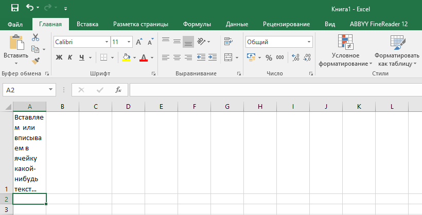
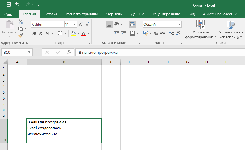
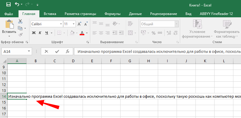
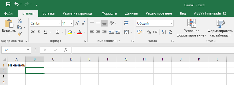
Приступая к работе в Microsoft Excel без должной подготовки, пользователь неизбежно столкнется с определенными трудностями, которые специалисту покажутся пустяковыми. Взять, к примеру, такую простую на первый взгляд операцию как перенос текста в ячейке. Пока вы набираете текст, Excel автоматически расширяет его по горизонтали, длинный текст отображается поверх соседних ячеек. А можно ли сделать так, чтобы длинный текст переносился на следующую строку и оставался в той же самой ячейке? Конечно можно, что мы сейчас и продемонстрируем.
Перенос текста в одной ячейке Excel
У нас есть некий длинный текст, который мы хотим разместить в одной ячейке, но так, чтобы он был видим целиком. Мы предложим два варианта размещения текста: без объединения ячеек и с объединением оных. Начнем с первого.
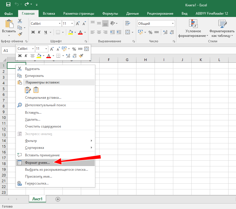
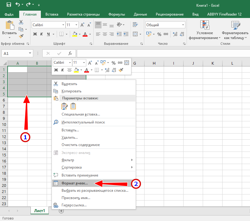
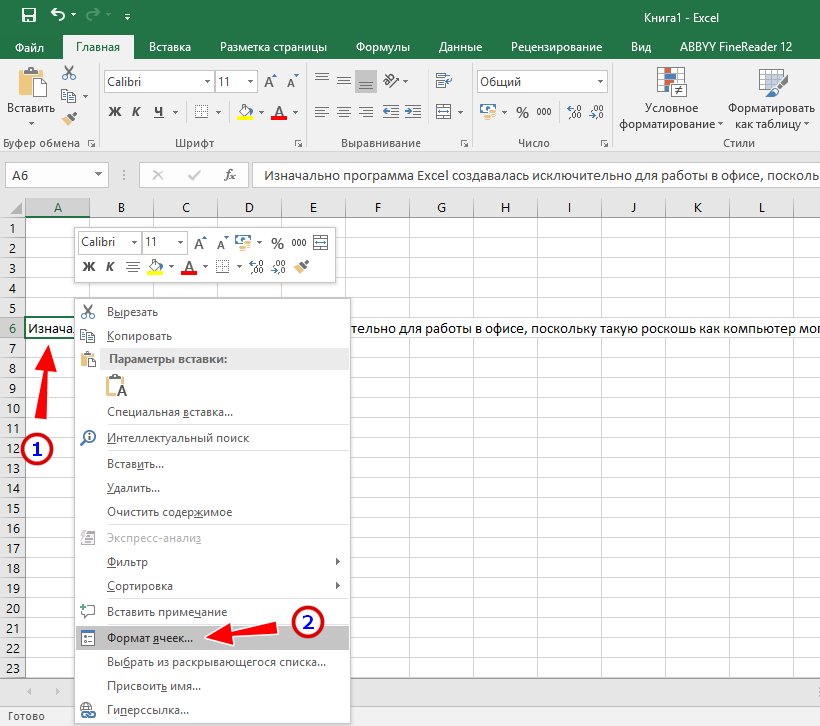
- Выделите ячейку мышкой, нажмите по выделенной области правой кнопкой мыши и выберите «Формат ячеек»;
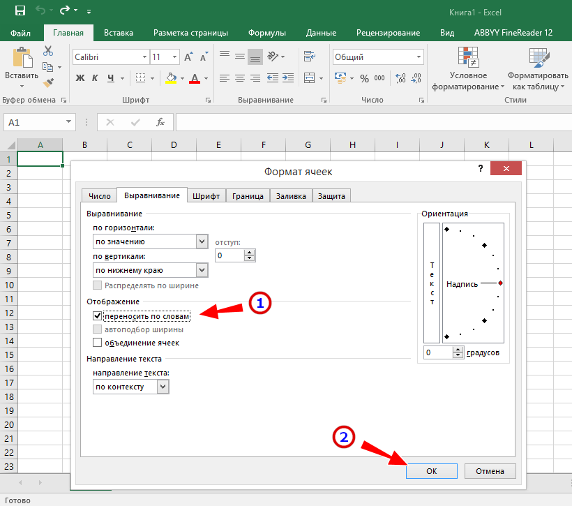
В открывшемся окне настроек на вкладке «Выравнивание» отметьте пункт «переносить по словам» и нажмите «OK»;
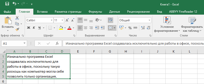
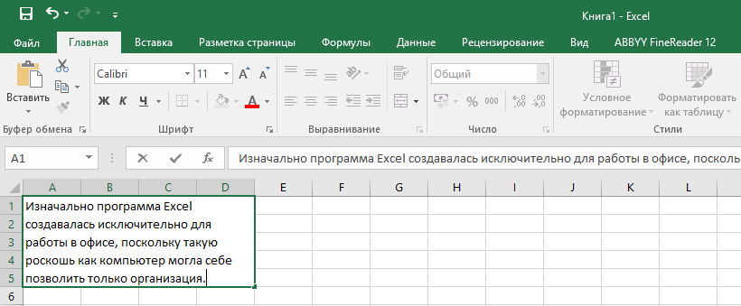
Сохранив настройки, можете смело набирать текст в созданной ячейке, не используя символ каретки;
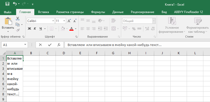
По завершении ввода нажмите Enter . Текст будет сохранен в одной ячейке и останется виден целиком, а ячейка растянется по высоте.
А вот и второй, более простой способ сделать автоперенос текста в ячейке.
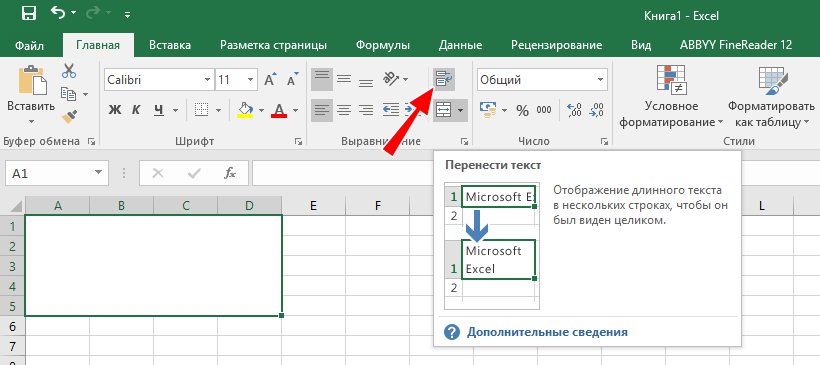
- Выделите мышкой ячейку, затем на панели инструментов, в блоке «Выравнивание» нажмите пиктограмму «Перенести текст» (смотрите скриншот);
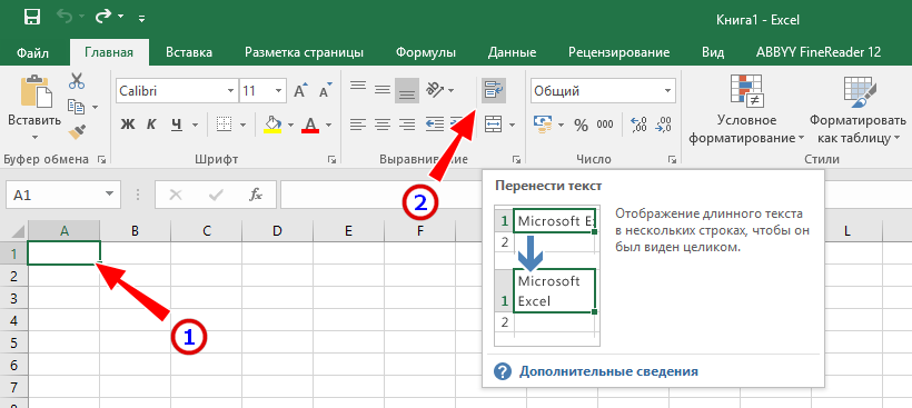
Всё готово, набирайте в ячейке ваш текст, а Excel сама позаботится о переносе его на новую строку в той же ячейке;
Нажмите Enter для сохранения результатов.
Перенос текста в объединенных ячейках Excel
А теперь рассмотрим способ вставки текста с переносом в объединенные ячейки. Для чего это нужно? Всё очень просто: вам может понадобиться крупная ячейка «на фоне» маленьких ячеек, используемых в Excel по умолчанию.
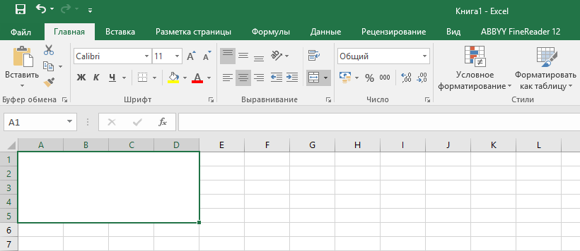
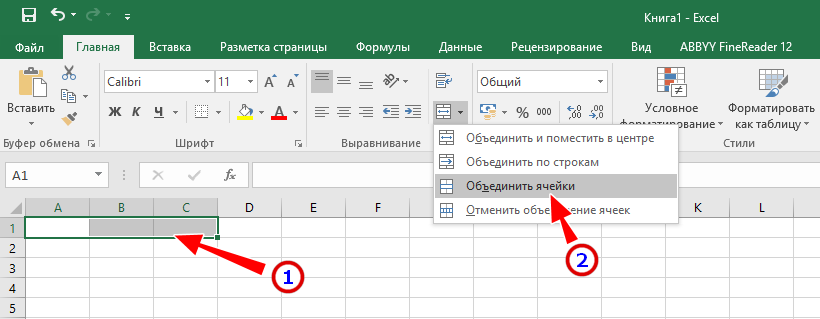
- Выделите мышкой или с помощью комбинации Shift + Стрелки нужное количество ячеек;
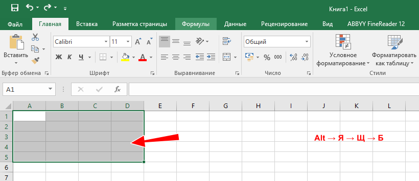
Нажмите последовательно клавиши Alt → Я → Щ → Б (необязательно с включенным капсом), вследствие чего ячейки тут же будут объединены;
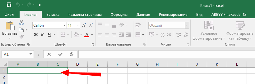
Нажмите на панели инструментов уже знакомую вам пиктограмму «Перенести текст»;
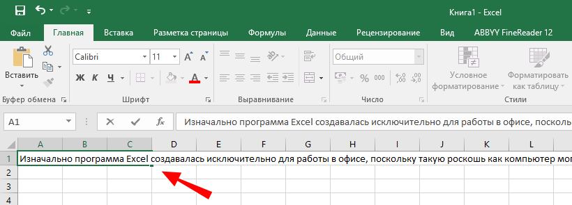
Вставьте в созданную ячейку ваш текст.
Тот же результат можно получить следующим образом:
- Выделите требуемое количество ячеек, кликните по выделенной области и выберите в меню опцию «Формат ячеек»;
В открывшемся окне отметьте чекбоксы «переносить по словам» и «объединение ячеек»;
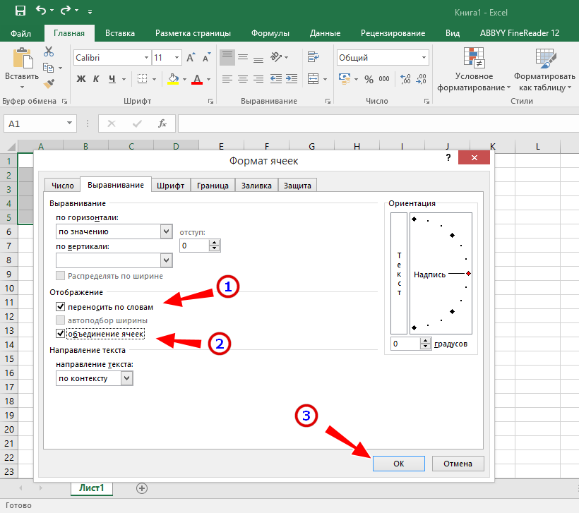
Нажмите «OK» и вставьте в ячейку ваш текст.
Как сделать перенос строки в ячейке Excel
С помощью «горячих клавиш»
Самым простым способом переноса текста внутри ячейки Excel является использование комбинации Alt + Enter .
- Установите курсор в ячейку и начинайте вводить текст;
- В том месте, где вы хотите сделать перенос, нажмите Alt + Enter и продолжайте вводить текст с новой строки;
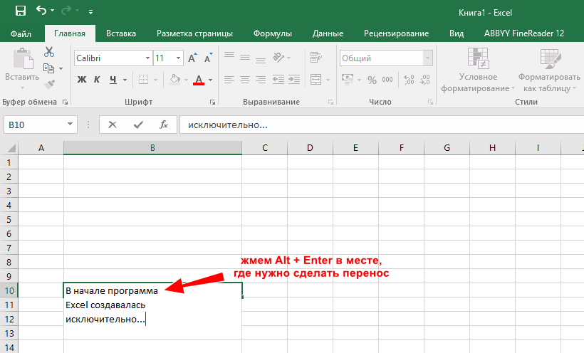
Завершив ввод текста, нажмите ввод. В результате вы увидите весь ваш текст в одной ячейке.
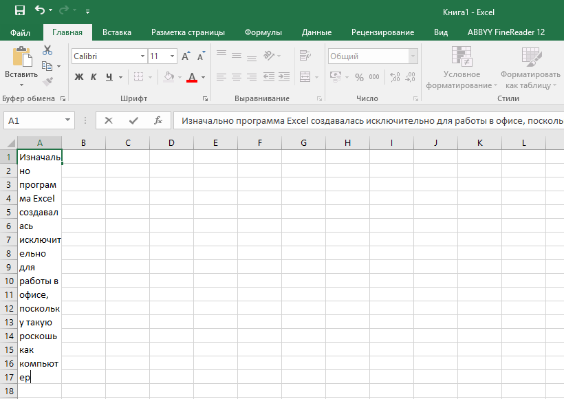
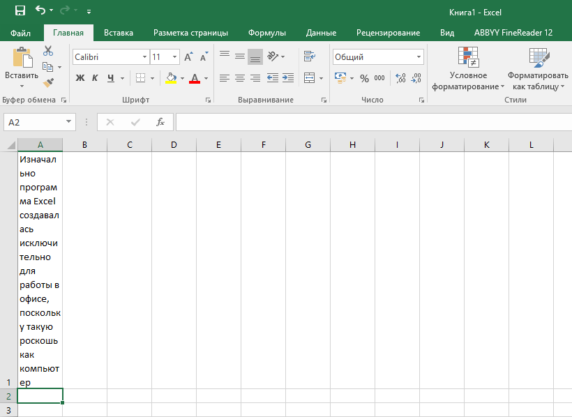
При переносе текста на новую строку с помощью клавиш в ячейке автоматически включается режим «Перенос текста». Чтобы увидеть результат ручного переноса, ширина столбца, в котором находится ячейка, должна быть достаточной, чтобы в ней уместилась фраза целиком до момента переноса, иначе сработает автоперенос по ширине ячейки и результат будет отличаться от ожидаемого
Перенос строки в ячейке Excel формулой
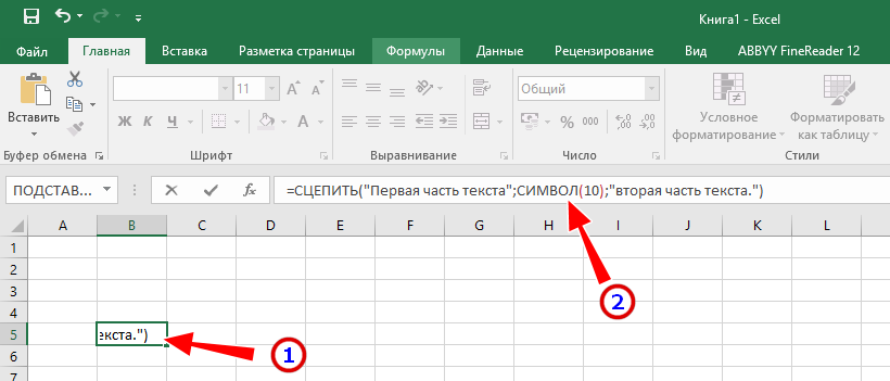
Для переноса текста в ячейках можно также использовать готовые формулы, например, формулу сцепления текста. Она имеет следующий формат:
Где СИМВОЛ(10) — это специальный невидимый символ переноса на новую строку, добавляемый между частями текста. К слову, когда вы нажимаете Alt + Enter , тот же символ переноса добавляется в конце строки. Заключенный в двойные кавычки текст может быть произвольным, это 2 фразы, которые должны быть расположены на разных строках внутри одной ячейки.
- Выделите ячейку, вставьте в поле формул указанную формулу с подготовленным текстом и нажмите ввод;
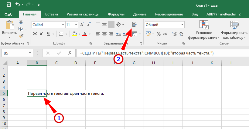
После того объединенный текст будет вставлен, выделите первую ячейку с началом текста и нажмите на панели инструментов кнопку переноса строк, иначе спецсимвол не будет работать;
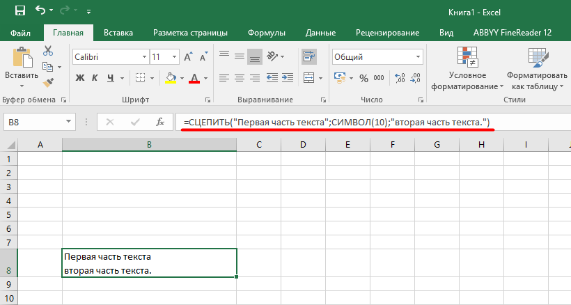
В результате вторая часть текста будет перенесена в ячейке на новую строку.
Как скрыть длинный текст в ячейке Excel
А сейчас мы рассмотрим обратную ситуацию, когда вставленный в ячейку более или менее объемный текст нужно частично скрыть, но таким образом, чтобы в нужный момент времени его можно было увидеть целиком. Делается это очень просто.
- Выделите ячейку и вставьте в нее свой текст так, как есть. Он растянется по всей длине ячеек;
Нажмите ввод, выделите первую ячейку, в которой хотите оставить видимый текст, нажмите по ней правой кнопкой мыши и выберите в контекстном меню опцию «Формат ячеек»;
В открывшемся окне переключитесь на вкладку «Выравнивание», в выпадающем списке «По горизонтали» выберите значение «с заполнением».
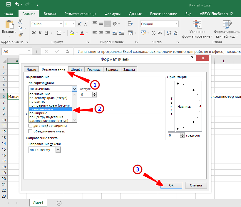
Теперь длинный текст будет скрыт, его отображение ограничится шириной текущей ячейки.
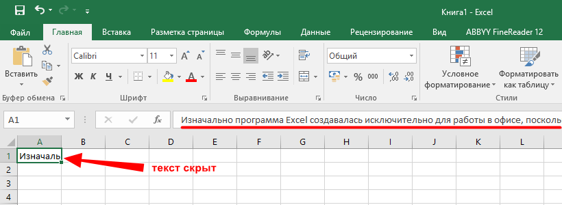
Чтобы увидеть текст целиком, нажмите на ячейку с фрагментом текста. Одинарное нажатие отобразит его только в поле ввода формул, двойной клик — в поле для формул и по всей длине ячеек.
А вот и альтернативный способ.
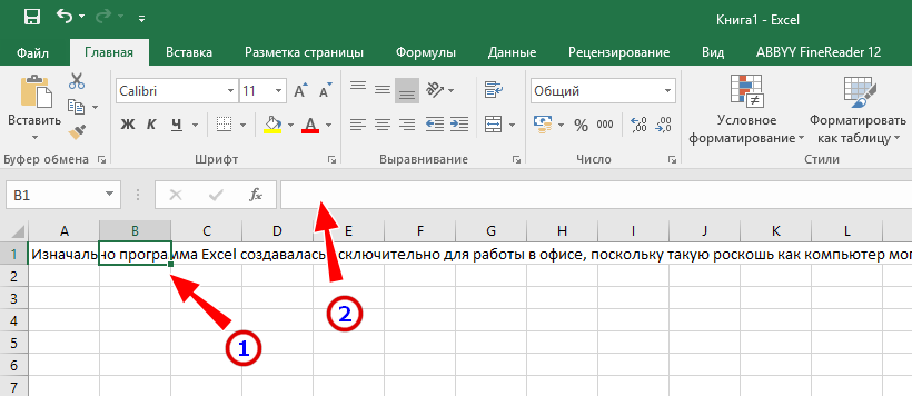
- Выделите ячейку и вставьте в нее свой текст так, как есть. Естественно, он растянется по всей длине ячеек;
Выделите соседнюю, заполненную частью текста ячейку и установите курсор в поле для вставки формул;
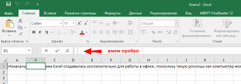
После того как выделенная ячейка станет пустой, нажмите пробел, а затем ввод. Лишний текст тут же будет скрыт, останется лишь его фрагмент в первой ячейке;
Если вы хотите видеть немного больше скрытой информации, можете воспользоваться таким способом.
- Объедините две или три ячейки с помощью инструмента «Объединить ячейки»;
Вставьте в удлиненную ячейку длинный текст и нажмите ввод. Лишний текст будет тут же скрыт;
Ну вот, теперь вы знаете, как можно быстро и без головной боли перенести текст на другую строку в ячейке программы Эксель или спрятать его основную часть. Однако, простота приведенных здесь примеров не должна вводить вас в заблуждение: этот программный компонент Microsoft Office довольно специфичен, и чтобы изучить все его возможности, нужно потратить не одну неделю.
Источник
How to wrap text in Excel
 by Svetlana Cheusheva, updated on February 7, 2023
This tutorial shows how to wrap text in a cell automatically and how to insert a line break manually. You will also learn the most common reasons for Excel wrap text not working and how to fix it.
Primarily, Microsoft Excel is designed to calculate and manipulate numbers. However, you may often find yourself in situations when, in addition to numbers, large amounts of text need to be stored in spreadsheets. In case longer text does not fit neatly in a cell, you can of course proceed with the most obvious way and simply make the column wider. However, it’s not really an option when you work with a large worksheet that has a lot of data to display.
A much better solution is to wrap text that exceeds a column width, and Microsoft Excel provides a couple of ways to do it. This tutorial will introduce you to the Excel wrap text feature and share a few tips to use it wisely.
What is wrap text in Excel?
When the data input in a cell is too large fit in it, one of the following two things happens:
- If columns to the right are empty, a long text string extends over the cell border into those columns.
- If an adjacent cell to the right contains any data, a text string is cut off at the cell border.
The screenshot below shows two cases: 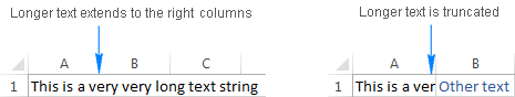
The Excel wrap text feature can help you fully display longer text in a cell without it overflowing to other cells. «Wrapping text» means displaying the cell contents on multiple lines, rather than one long line. This will allow you to avoid the «truncated column» effect, make the text easier to read and better fit for printing. In addition, it will help you keep the column width consistent throughout the entire worksheet.
The following screenshot shows how wrapped text looks like in Excel: 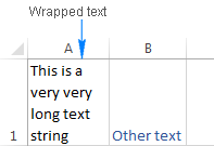
How to wrap text in Excel automatically
To force a lengthy text string to appear on multiple lines, select the cell(s) that you want to format, and turn on the Excel text wrap feature by using one of the following methods.
Method 1. Go to the Home tab > Alignment group, and click the Wrap Text button: 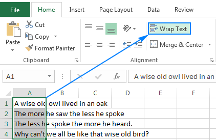
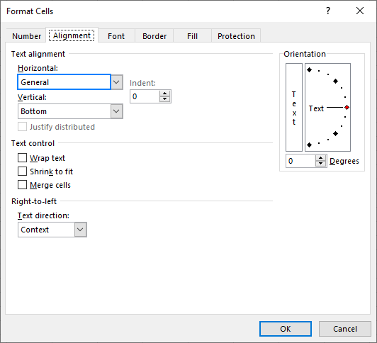
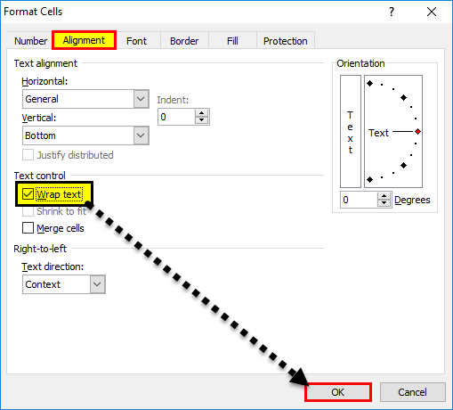
Method 2. Press Ctrl + 1 to open the Format Cells dialog (or right-click the selected cells and then click Format Cells…), switch to the Alignment tab, select the Wrap Text checkbox, and click OK. 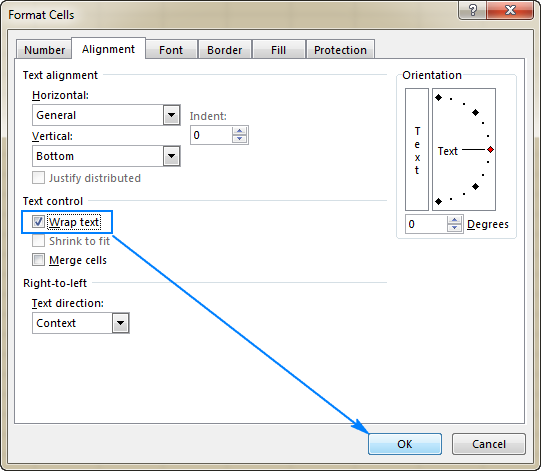
Compared to the first method, this one takes a couple of extra clicks, but it may save time in case you wish to make a few changes in cell formatting at a time, wrapping text being one of those changes.
Tip. If the Wrap Text checkbox is filled in solid, it indicates that the selected cells have different text wrap settings, i.e. in some cells the data is wrapped, in other cells it is not wrapped.
Result. Whichever method you use, the data in the selected cells wraps to fit the column width. If you change the column width, text wrapping will adjust automatically. The following screenshot shows a possible result: 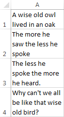
How to unwrap text in Excel
As you can easily guess, the two methods described above are also used to unwrap text.
The fastest way is to select the cell(s) and click the Wrap Text button (Home tab > Alignment group) to toggle text wrapping off.
Alternatively, press the Ctrl + 1 shortcut to open the Format Cells dialog and clear the Wrap text checkbox on the Alignment tab.
How to insert a line break manually
Sometimes you may want to start a new line at a specific position rather than have lengthy text wrap automatically. To enter a line break manually, just do the following:
- Enter cell edit mode by pressing F2 or double-clicking the cell or clicking in the formula bar.
- Put the cursor where you want to break the line, and press the Alt + Enter shortcut (i.e. press the Alt key and while holding it down, press the Enter key).
Result. Inserting a manual line break turns on the Wrap Text option automatically. However, the line breaks entered manually will stick in place when the column is made wider. If you turn off text wrapping, the data displays in one line in a cell, but the inserted line breaks are visible in the formula bar. The following screenshot demonstrates both scenarios — a line break in entered after the word «owl. 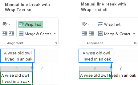
For other ways to insert a line break in Excel, please see: How to start a new line in a cell.
Excel wrap text not working
As one of the most often used features in Excel, Warp Text was designed as simple as possible and you will hardly have any problems using it in your worksheets. If text wrapping does not work as expected, check out the following troubleshooting tips.
1. Fixed row height
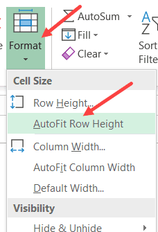
If not all wrapped text is visible in a cell, most likely the row is set to a certain height. To fix this, select the problematic cell, go to the Home tab > Cells group, and click Format > AutoFit Row Height: 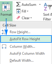
Or, you can set a specific row height by clicking Row Height… and then typing the desired number in the Row height box. A fixed row height comes in especially handy to control the way the table headers are displayed.
2. Merged cells
Excel’s Wrap Text does not work for merged cells, so you will have to decide which feature is more important for a particular sheet. If you keep the merged cells, you can display the full text by making the column(s) wider. If you opt for Wrap Text, then unmerge cells by clicking the Merge & Center button on the Home tab, in the Alignment group: 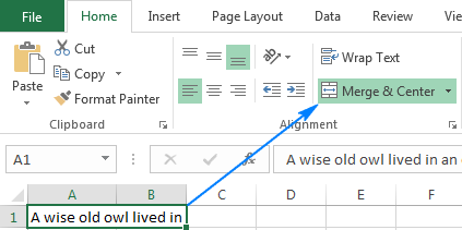
3. The cell is wide enough to display its value
If you try to wrap a cell(s) that is already wide enough to display its contents, nothing will happen, even if later on the column is resized and becomes too narrow to fit longer entries. To force the text to wrap, toggle the Excel Wrap Text button off and on again.
4. Horizontal alignment is set to Fill
Sometimes, people want to prevent text from spilling over into next cells. This can be done by setting Fill for horizontal alignment. If later on you enable the Wrap Text feature for such cells, nothing will change — text will still be truncated at the cell’s boundary. To resolve the issue, remove the Fill alignment:
- On the Home tab, in the Alignment group, click the Dialog launcher (a small arrow in the lower-right corner of a ribbon group). Or press Ctrl + 1 to open the Format Cells dialog box.
- On the Alignment tab of the Format Cells dialog box, set General for Horizontal alignment, and click OK.
This is how you wrap text in Excel to display longer text on multiple lines. I thank you for reading and hope to see you on our blog next week!
Источник
-
04-08-2005, 09:06 AM
#1
Why doesn’t text wrap in a cell in Excel?
I am typing text in a cell and want it to wrap. I checked «wrap text» box
however it still doesn’t wrap and I can only see part of the text. When I
click on the cell the text is there, but I still can’t view it if I’m not in
that specific cell.
-
04-08-2005, 09:06 AM
#2
Re: Why doesn’t text wrap in a cell in Excel?
Is your cell high enough? Try making your cell hight a bit taller. Excel
should automatically adjust the cell height, but that’s not always the case.X_HOBBES
«rohrbaught» <rohrbaught@discussions.microsoft.com> wrote in message
news:ED2C5BEC-FA41-4257-88CB-C348E718A529@microsoft.com…
> I am typing text in a cell and want it to wrap. I checked «wrap text» box
> however it still doesn’t wrap and I can only see part of the text. When I
> click on the cell the text is there, but I still can’t view it if I’m not
in
> that specific cell.
-
04-08-2005, 10:06 AM
#3
Re: Why doesn’t text wrap in a cell in Excel?
Move the mouse to the row number on the left and double-clik on the
bottom border. The row height will auto adjust.
-
04-08-2005, 10:06 AM
#4
Re: Why doesn’t text wrap in a cell in Excel?
rohrbaught shared this with us in microsoft.public.excel.misc:
> I am typing text in a cell and want it to wrap. I checked «wrap
> text» box however it still doesn’t wrap and I can only see part of
> the text. When I click on the cell the text is there, but I still
> can’t view it if I’m not in that specific cell.Press ALT+Enter to insert new lines in the same cell.
—
Amedee Van Gasse using XanaNews 1.17.3.1
If it has an «X» in the name, it must be Linux?How To Ask Questions The Smart Way
http://www.catb.org/~esr/faqs/smart-questions.html
How to Report Bugs Effectively
http://www.chiark.greenend.org.uk/~sgtatham/bugs.html
Only ask questions with yes/no answers if you want «yes» or «no» as the
answer.
http://homepages.tesco.net/~J.deBoyn…-with-yes-or-n
o-answers.html
-
04-08-2005, 10:06 AM
#5
Re: Why doesn’t text wrap in a cell in Excel?
You are exactly right…I expanded the height with my cursor and sure enough
the «hidden» text appeared. Thanks!«X_HOBBES» wrote:
> Is your cell high enough? Try making your cell hight a bit taller. Excel
> should automatically adjust the cell height, but that’s not always the case.
>
> X_HOBBES
>
>
> «rohrbaught» <rohrbaught@discussions.microsoft.com> wrote in message
> news:ED2C5BEC-FA41-4257-88CB-C348E718A529@microsoft.com…
> > I am typing text in a cell and want it to wrap. I checked «wrap text» box
> > however it still doesn’t wrap and I can only see part of the text. When I
> > click on the cell the text is there, but I still can’t view it if I’m not
> in
> > that specific cell.
>
>
>
-
04-08-2005, 10:06 AM
#6
Re: Why doesn’t text wrap in a cell in Excel?
Sorry, I wasn’t able to follow your instructions.
«P Sitaram» wrote:
> Move the mouse to the row number on the left and double-clik on the
> bottom border. The row height will auto adjust.
>
>
-
04-08-2005, 10:06 AM
#7
Re: Why doesn’t text wrap in a cell in Excel?
Thanks for responding…I tried this and did not work.
«Amedee Van Gasse» wrote:
> rohrbaught shared this with us in microsoft.public.excel.misc:
>
> > I am typing text in a cell and want it to wrap. I checked «wrap
> > text» box however it still doesn’t wrap and I can only see part of
> > the text. When I click on the cell the text is there, but I still
> > can’t view it if I’m not in that specific cell.
>
> Press ALT+Enter to insert new lines in the same cell.
>
> —
> Amedee Van Gasse using XanaNews 1.17.3.1
> If it has an «X» in the name, it must be Linux?
>
> How To Ask Questions The Smart Way
> http://www.catb.org/~esr/faqs/smart-questions.html
> How to Report Bugs Effectively
> http://www.chiark.greenend.org.uk/~sgtatham/bugs.html
> Only ask questions with yes/no answers if you want «yes» or «no» as the
> answer.
> http://homepages.tesco.net/~J.deBoyn…-with-yes-or-n
> o-answers.html
>
-
04-08-2005, 11:06 AM
#8
Re: Why doesn’t text wrap in a cell in Excel?
rohrbaught shared this with us in microsoft.public.excel.misc:
> Thanks for responding…I tried this and did not work.I’m sorry to hear that. It works for me.
Please note that this does not make the line wrap, it just adds hard
coded line breaks. Please follow Hobbes’ instructions.—
Amedee Van Gasse using XanaNews 1.17.3.1
If it has an «X» in the name, it must be Linux?How To Ask Questions The Smart Way
http://www.catb.org/~esr/faqs/smart-questions.html
How to Report Bugs Effectively
http://www.chiark.greenend.org.uk/~sgtatham/bugs.html
Only ask questions with yes/no answers if you want «yes» or «no» as the
answer.
http://homepages.tesco.net/~J.deBoyn…-with-yes-or-n
o-answers.html
-
04-08-2005, 02:06 PM
#9
Re: Why doesn’t text wrap in a cell in Excel?
You also need to make sure your cell is set to wrap. Right click on
cell. Click format. Alignment tab. Check «Wrap Text»
-
04-19-2005, 12:57 PM
#10
Registered User
Merged cells cause the problem…
…try putting a single cell to the right (of width equal to the sum of all the merged cells with the wrap problem and with word wrap ticked — best to format the same).
Then make this cell equal the merged cell (e.g. «=C3»).
The autofit should now work.
-
08-09-2016, 01:09 PM
#11
Registered User
Re: Why doesn’t text wrap in a cell in Excel?
I had similar problem. I had a table with many columns and rows with text. Wrap text option didn’t work but I wanted to print directly from Excel.
My solution was this. I selected whole column and clicked Wrap text button and it WORKED. I tried to select more columns at same time and it WORKED. When I select whole table it didn’t work.
-
12-31-2017, 01:15 PM
#12
Registered User
Re: Why doesn’t text wrap in a cell in Excel?
I tried all of the suggested fixes and none worked for me. My worksheet had data that was converted from a pdf spreadsheet. It had cells that been merged, then unmerged and text Concantonated, date times split to date column and time columns, etc.
I even had some cells in a column where the text would center ok and the in the next row the text would not center no matter what formatting I tried.
The only thing that ended up working was to:
1) Save the sheet as a comma delineated file.
2) Close it.
3) Open it.
It now has all the data back in default formatting — no wrapping, not autofit.I was then able to select columns and set Word Wrap. Select other columns and select Autofit. Select the entire worksheet and Autofit rows. Change fonts and font sizes.
-
11-11-2018, 11:23 PM
#13
Registered User
Re: Why doesn’t text wrap in a cell in Excel?
I had the same problem. First, select the all the cells you’re having the issue with. Then click Home tab. Then click Format tab. Then select row, then autofit.
This worked for me. Now all the rows show the wrapped text.


What is Wrap Text in Excel?
The wrap text feature in excel allows displaying lengthy text strings of a cell in multiple lines. This enhances the readability of the worksheet and ensures that the entire cell data is visible at all times. After wrapping text, the row height increases automatically though the column width stays the same. If one changes the column width, the cell content adjusts itself to fit the new width.
For example, in the following image, wrap text has been applied to the string in cell B2. At the same time, column B has been widened.
The purpose of wrapping text is to prevent the cell data from spilling to the cells on the right. Moreover, it ensures that a text string is not cut by the border of the adjacent cell. Wrapping text is extremely helpful in worksheets that have a lot of content to display at a time.
Table of contents
- What is Wrap Text in Excel?
- How to Wrap the Text in Excel?
- Method #1–Using the Home tab
- Method #2–Using the “Format Cells” Window
- Method #3–Using the Keyboard Shortcut
- Method #4–Using Line Breaks
- The Reasons “Wrap Text” Feature may not Work in Excel
- Frequently Asked Questions
- Recommended Articles
- How to Wrap the Text in Excel?
How to Wrap the Text in Excel?
Wrap text is a formatting feature of Excel, which changes the appearance of a string without changing the string itself. The methods of wrapping text are listed as follows:
- Method #1–Wrap text using the Home tab
- Method #2–Wrap text using the “format cells” window
- Method #3–Wrap text using the keyboard shortcut
- Method #4–Wrap text using line breaks
Note that methods #1 to #3 wrap text automatically, while method #4 wraps text manually. In method #4, line breaks are inserted at the desired place in a cell. A line break serves as a substitute for the wrap text feature of Excel.
Let us discuss the four methods with the help of examples.
You can download this Wrap Text Excel Template here – Wrap Text Excel Template
Method #1–Using the Home tab
The succeeding image shows a long text string in cell A2. We want to wrap this text in cell A2. Use the “wrap text” option of the Home tab.
The steps to wrap text in excel by using the stated method are listed as follows:
Step 1: Select cell A2 whose text string needs to be wrapped.
Step 2: From the “alignment” group of the Home tab, click “wrap text.” The text string of cell A2 is displayed in multiple lines, as shown in the succeeding image.
Notice that even after wrapping text, the width of column A stays the same as that of the other columns. However, the height of row 2 increases when this feature is turned on.
Note 1: “Wrap text” is a toggle button that can be turned on and off to wrap and unwrap the text.
Note 2: To wrap the text of multiple cells simultaneously, select all such cells and press the “wrap text” toggle button.
Method #2–Using the “Format Cells” Window
Working on the text string of method #1, we want to wrap the text in cell A2. Use the “format cells” window of Excel.
The steps to wrap text in excel by using “Format Cells” are listed as follows:
- Select cell A2 containing the string to be wrapped. Right-click the selection and choose “format cells” from the context menu.
Alternatively, press the shortcut “Ctrl+1” after selecting the cell.

- The “format cells” window opens, as shown in the following image. Click the “alignment” tab. Then, from “text control,” choose the “wrap text” option and click “Ok.”

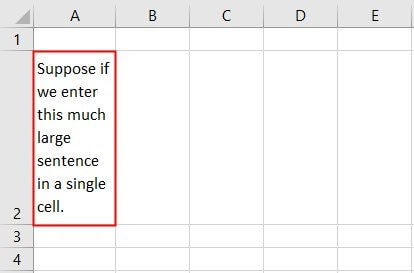
- The wrap text feature has been applied to cell A2, as shown in the following image. This time also, the width of column A has not changed, but the height of row 2 has increased.

Method #3–Using the Keyboard Shortcut
The succeeding image shows a text string in cell A1. We want to wrap this string of cell A1. Use the keyboard shortcutAn Excel shortcut is a technique of performing a manual task in a quicker way.read more for wrapping text.
The steps to wrap text in excel by using keyboard shortcut are listed as follows:
Step 1: Select cell A1 that consists of the string to be wrapped.
Step 2: Press the shortcut keys “Alt+H+W.” For this shortcut to work, first press the “Alt” key and release it. Next, press and release the “H” key followed by the “W” key.

Step 3: Once the “W” key is released, the “wrap text” feature is applied to the cell selected in step 1. The output is shown in the following image.
Method #4–Using Line Breaks
Working on the text string of method #1, we want to perform the following tasks:
- Apply the wrap text feature in cell A1.
- Insert line breaks manually after the strings “enter,” “large,” and “a” in cell A2.
- Compare the results of applying wrap text with inserting line breaks.
Use the keyboard shortcut for inserting line breaks. Note that both cells A1 and A2 should contain the text string of method #1.
The steps to perform the given tasks are listed as follows:
Step 1: Wrap the text in cell A1 by selecting the cell and choosing “wrap text” from the Home tab. The output is shown in cell A1 of the succeeding image.
Step 2: To insert line breaks, place the cursor in that part of the cell where line breaks are to be inserted. Next, press the keys “Alt+Enter” together.
So, first, place the cursor after the string “enter” and press the given shortcut. The line break is inserted at the end of this string. Likewise, insert line breaks after the strings “large” and “a.”
The result is shown in cell A2 of the following image.
Comparison between applying wrap text and inserting line breaks: It must be noted that when a line break is inserted, the “wrap text” feature is automatically turned on in Excel.
Therefore, when “wrap text” is applied, it is applied alone. However, when a line break is added, it is added in combination with “wrap text.”
The line breaks entered in cell A2 will stay in place even if column A is made wider. Moreover, if “wrap text” is turned off but the line breaks are retained, the string of cell A2 appears in a single line. However, the line breaks inserted in step 2 are visible in the formula bar.
In contrast, when the “wrap text” of cell A1 is disabled, the string appears as a single line, in this cell and the formula bar. So, with wrap text in excel, the cell content can regain its initial appearance with a single click of the toggle button.
The Reasons “Wrap Text” Feature may not Work in Excel
The reasons due to which the wrap text feature may not work in Excel are listed as follows:
- It does not work on merged cells. So, cells need to be unmerged before the wrap text feature can be applied to them.
- It does not work if the cell is already wide enough to display the entire text string. In this case, one can insert line breaks to display the cell content in multiple lines.
- It may not be visible if the height of the row has been set at a very low value. To avoid this, make sure that the height of the row adjusts automatically with the application of the wrap text feature in excel.
Note: To ensure that wrapped text is visible at all times, follow either of the listed techniques in Excel:
- Set the row height to adjust automatically. For this, click the “format” drop-down from the “cells” group of the Home tab. Next, choose “AutoFit row height” from the “cell size” option.
- Enlarge the height of the row manually. For this, place the cursor on the lower border of the row label. The row labels are displayed on the left side of the worksheet. Once the “resizing” mouse pointer appears, drag the lower border of the row downwards to increase the row height.
Frequently Asked Questions
1. What is the wrap text feature and where is it in Excel?
The wrap text feature in excel helps display the content of a cell in multiple lines. With wrap text, the text is wrapped in such a way that the row height increases, but the column width stays the same. Further, the column width can be increased or decreased by the user. The text string adjusts itself automatically with a change in the column width.
However, even after applying the wrap text feature, one can maintain a consistent column width throughout the worksheet. The “wrap text” is a toggle button of Excel, which is available in the “alignment” group of the Home tab.
Note: For more details on the working of the wrap text feature, refer to the examples of this article.
2. List the reasons and state the shortcut of using the wrap text feature in Excel.
The wrap text feature is used in Excel for the following reasons:
• To prevent text strings from being truncated by the adjacent cell
• To avoid overlapping of text strings
• To ensure that the entire cell content is visible
• To improve the readability of large datasets
• To make the worksheet neat, organized, and fit for printing
In Excel, the shortcut of wrapping text is “Alt+H+W.” All the keys must be pressed one after the other in the given sequence. Prior to using this shortcut, ensure that the cell, whose text is to be wrapped, is selected.
3. How to wrap text without expanding the size of the cell in Excel?
After applying the wrap text feature, one can keep either the row height or the column width constant but not both simultaneously. If both (row height and column width) are held constant, the wrapped text will not be visible.
The steps to keep the row height constant are listed as follows:
• Select the cell in which the text is to be wrapped.
• Click the “format” drop-down from the “cells” group of the Home tab.
• From “cell size,” select “row height.”
• In the “row height” window, do not enter any value. Simply click “Ok.”
Now, when the wrap text feature is applied to the selected cell, the row height will remain the same as that of the other rows. On the other hand, the column width already stays constant even after applying the wrap text feature.
However, when the text of a cell is wrapped, it is recommended that one should not prevent a cell from expanding. This is because the basic purpose of wrap text will not be served if the cell is not permitted to enlarge.
Recommended Articles
This has been a guide to wrap text in Excel. Here we discuss how to wrap text in Excel by using the top 4 methods along with shortcuts and examples. You may also look at these useful functions in Excel–
- Format Text in ExcelText formatting in Excel include changing the colour, font name, font size, alignment, font appearance in bold, underlining, italic, background colour of the font cell, and so on.read more
- Separating Text in ExcelThe methods used to separate text in Excel are as follows: 1) Text to Column (Delimited and Fixed Width) 2) Using Excel Formulasread more
- Add Text in Excel FormulaText in Excel Formula allows us to add text values to using the CONCATENATE function or the ampersand (&) symbol.read more
- Change Case in ExcelPROPER, UPPER, and LOWER are the three Excel functions that help in converting the text to proper case, upper case and lower case respectively.read more
A quick look at an Excel sheet can tell you that the regular size of a cell is a decent fit for numbers but for this tutorial, we are more concerned about a cell’s fit for text. With an acceptable font size, fitting 7-8 characters in a cell is no problem. For fitting more than one word in, there is no need to resort to a different column or row or keep adjusting with Alt + Enter. You have Word Wrap at your service.
Type all the text in a cell. Hit Enter. You will notice the text sprawled all the way to the cells on the right. If the cells on the right are preoccupied, the text will seem to hide behind the preoccupied cells. If you don’t mind expanding the column width to accommodate all the text, adjust the column width or double click the column width in the column header and Bob’s your uncle.
But if we don’t want Bob as our uncle and want to compact the text to be displayed completely in one cell without compromising on column width, we wrap the text. When we say «we wrap the text», we don’t really do anything strenuous; Excel is more than willing to do it for us. The options are simple, one of which requires a single click.
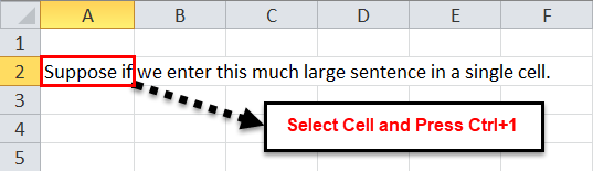
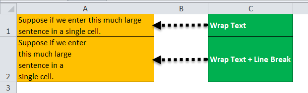
 1")
What happens when the text is wrapped? The text compacts into the cell it was originally written in with no impact on the column width but increased row height.
See how the text looks before and after wrapping:
 2")
Let’s find out how to do this.
Apply Wrap Text from Ribbon
Step 1, click on the Wrap Text button. The end. Really!
See if you can figure out the problem here:
 3")
That is one delicious receipt but the longer item names are hiding behind the next column. Being a receipt, we’d like to keep it this compact. Hence, instead of extending the column width, we will wrap the text like this:
- Select the cell(s) for word wrapping. We will select column B.
- From the Home tab, in the Alignment group, click on the Wrap Text command button.
 4")
Consider the text wrapped! Once Wrap Text is applied, any text entered in the text-wrapped cells will automatically be wrapped. E.g. since we have applied Wrap Text to column B. Any text added later to column B will be wrapped.
 5")
Sometimes Wrap Text may break the words while wrapping (Some letters of the word in the top line and the rest in the bottom line), in which case you will need to adjust the column width or adjust the words. To manually shift text to the next line, position the blinking cursor at the start of the text to be shifted and press Alt + Enter.
Apply Wrap Text from the Format Cells Dialog Box
Any cell formatting option is incomplete without a nod to the Format Cells dialog window. Text can be wrapped using the Format Cells dialog box which is a few more clicks than the previous method but simple nonetheless. This option is useful especially if you’re already using the Format Cells dialog box; might as well wrap some text while you’re at it. Here are the steps:
- Select the cell(s) for word wrapping. We will select column B.
- Right-click the selected cells. Select Format Cells from the context menu to launch the Format Cells dialog box (or use the keyboard shortcut Ctrl + 1 or click the dialog launcher arrow in the Alignment group under the Home).
 6")
- In the Format Cells dialog box, select the Alignment In the Text control group, check the Wrap Text tick box.
- Click OK.
 7")
Text is wrapped! Once Wrap Text is applied, any text entered in the text-wrapped cells will automatically be wrapped. E.g. since we have applied Wrap Text to column B. Any text added later to column B will be wrapped.
Apply Wrap Text Using Keyboard Shortcut
Press the keys one after the other to apply the shortcut keys for Wrap Text:
Alt H W
- Pressing Alt will display the shortcut key for each tab on the sheet.
- H selects the Home tab and further displays other shortcut keys for the commands on the ribbon menu.
- W will select the Wrap Text
Recommended Reading: How To Indent In Excel
Wrap Text Not Working
There are a few settings that may hinder wrapping text the right way. We have listed them below with ways to tackle them.
Fixed Row Height
Although Wrap Text is mostly about keeping the column width while expanding the row height to accommodate all the text in a cell, you may notice that sometimes the wrapped text is still being obstructed by insufficiently expanded row height. The reason for this is that the row height is preset to a certain height already and therefore will not expand further to display the complete text despite the Wrap Text feature applied.
Let’s suppose we have preset the row height to 40 pixels (which in our case is almost equivalent to the height of two lines) but we enter an item that will require three lines.
 9")
As you can spot in the Home tab’s Alignment group, Wrap Text has already been applied but hasn’t solved our problem of completely wrapping B6’s text into the cell. This is because we have preset the row height to 40 pixels, therefore the row height is not extending to the required 60 pixels.
We can double-click row 6’s row header but that would be a solution only for the text in row 6. For a sheet-wide solution, we can activate the AutoFit Row Height option. For our example, we only require this convenience for column B so we will only apply AutoFit Row Height to it instead of the whole sheet.
- Select the target text cells. We will select column B.
- Go to Home tab > Cells group > Format command button. Click the AutoFit Row Height
 10")
- This option will fit the row heights of all selected cells to display the complete text.
 11")
Do note that the AutoFit Row Height option will only apply with Wrap Text enabled. The beauty of AutoFit Row Height is that you wouldn’t have to keep a preset row height for the complete text to be displayed; the row height will autofit according to the height required for each cell’s text. Whereas with a preset row height, cells with lesser text will unnecessarily have more height too, needlessly expanding the size of the dataset.
Merged Cells
Wrap text will not apply to merged cells. Evidence below:
 12")
Until Excel finds a solution for this one, you’ll have to decide whether merged cells are a keeper or goner.
With merged cells: either adjust the column width or row height to display the complete text.
Without merged cells: Unmerge the cells from the Home tab, Alignment group, Merge & Center command button, Unmerge Cells option. Then adjust the column width or row height to display the complete text.
Horizontal Alignment is Set to Fill
The horizontal alignment of the text of a cell may be set to Fill to prevent it from spilling to the next cell(s). In this case, Wrap Text will not work. There would be no change in such cells when Wrap Text is applied. Here is what text wrapping would look like applied to General Horizontal Alignment and Fill Horizontal Alignment:
 13")
The solution is to remove the culprit; change the Horizontal Alignment of the text from Fill back to General. Here’s the way:
- Select the target text cells.
- Press Ctrl + 1 to open the Format Cells dialog box. You can also open the Format Cells dialog box from the right-click context menu or the dialog launcher arrow from the Alignment group in the Home
 14")
- In the Alignment tab, in the Text alignment section, change the Horizontal alignment from Fill to General.
- Click OK.
 15")
General Horizontal Alignment is the default setting and it quickly fixes this matter.
Recommended Reading: How to Rotate Text In Excel
Remove Wrap Text
The steps for removing Wrap Text are the same as the steps we used to apply it.
Removing Wrap Text Using Ribbon Menu
Select the desired cell or range of cells. Navigate to Home tab > Alignment group. The Wrap Text command button should be already highlighted denoting that it is already enabled.
Click the Wrap Text command button and the wrap text is disabled.
Removing Wrap Text Using Format Cells dialog box
Select the desired cell or range of cells. Launch the Format Cells dialog box (Ctrl + 1). Uncheck Wrap Text from the Alignment tab, Text control section, and click OK.
Removing Wrap Text Using Keyboard Shortcut
Press Alt H W one after the other.
All three ways above will remove Wrap Text from the cell(s).
It’s a wrap, everyone! We wrap up this guide with the hope that we made text wrapping and unwrapping easier for you to understand and apply. We’d like to see you around with another slither of Excel. Until then, keep Excel-erating!