
Excel for Microsoft 365 Excel 2021 Excel 2019 Excel 2016 Excel 2013 Excel 2010 Excel 2007 More…Less
Let’s say you want to ensure that a column contains text, not numbers. Or, perhapsyou want to find all orders that correspond to a specific salesperson. If you have no concern for upper- or lowercase text, there are several ways to check if a cell contains text.
You can also use a filter to find text. For more information, see Filter data.
Find cells that contain text
Follow these steps to locate cells containing specific text:
-
Select the range of cells that you want to search.
To search the entire worksheet, click any cell.
-
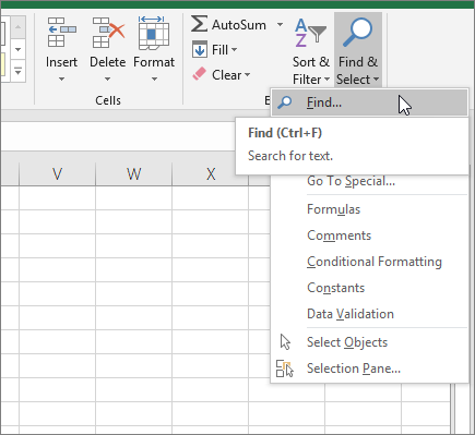
On the Home tab, in the Editing group, click Find & Select, and then click Find.

-
In the Find what box, enter the text—or numbers—that you need to find. Or, choose a recent search from the Find what drop-down box.
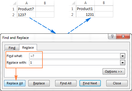
Note: You can use wildcard characters in your search criteria.
-
To specify a format for your search, click Format and make your selections in the Find Format popup window.
-
Click Options to further define your search. For example, you can search for all of the cells that contain the same kind of data, such as formulas.
In the Within box, you can select Sheet or Workbook to search a worksheet or an entire workbook.
-
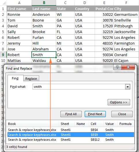
Click Find All or Find Next.
Find All lists every occurrence of the item that you need to find, and allows you to make a cell active by selecting a specific occurrence. You can sort the results of a Find All search by clicking a header.
Note: To cancel a search in progress, press ESC.
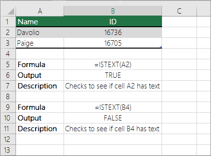
Check if a cell has any text in it
To do this task, use the ISTEXT function.
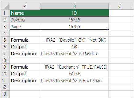
Check if a cell matches specific text
Use the IF function to return results for the condition that you specify.
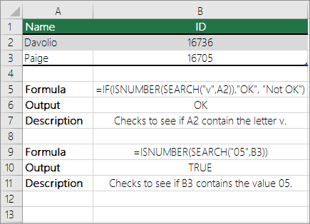
Check if part of a cell matches specific text
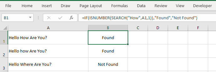
To do this task, use the IF, SEARCH, and ISNUMBER functions.
Note: The SEARCH function is case-insensitive.
Need more help?
Summary:
This informative post will help you to know why your Excel find and replace not working. Besides this, the post covers some best fixes to resolve “Microsoft Excel Cannot Find the Data You’re Searching For” error occurs mainly when Excel find and replace doesn’t work.
While working with huge Excel data, it’s too difficult and time consuming to search for any specific information. Well to simplify this task Excel has provided its user with find and replace features.
However, through the ‘Find’ option user can easily fetch any of their worksheet’s data whereas with the ‘replace’ feature you can make quick modifications to your worksheet.
Undoubtedly, these features simplify the working style in Excel a bit easier but what if Excel find and replace stops working.
Don’t know how to tackle such a situation in Excel? Not to worry…!
Let’s take a quick glance to uncover the unsolved mystery of Excel find and replace not working issue.
To recover lost Excel data, we recommend this tool:
This software will prevent Excel workbook data such as BI data, financial reports & other analytical information from corruption and data loss. With this software you can rebuild corrupt Excel files and restore every single visual representation & dataset to its original, intact state in 3 easy steps:
- Download Excel File Repair Tool rated Excellent by Softpedia, Softonic & CNET.
- Select the corrupt Excel file (XLS, XLSX) & click Repair to initiate the repair process.
- Preview the repaired files and click Save File to save the files at desired location.
What Happens When Excel Find And Replace Won’t Work?
Problem 1:
At the time using the Find utility to search for any specific Excel workbook data, you may start getting an error message like:
Microsoft Excel cannot find the data you’re searching for.
Check your search options, location and formatting.
Problem 2:
In the Microsoft Excel application when you select the Replace option from the dialog box of Find and Replace for replacing data already existing in your Excel worksheet. At that time, you may be stuck with the following error message:
Microsoft Excel cannot find a match.
It’s ok to get this “Microsoft Excel cannot find a match” error when the text that you need to replace actually won’t exist in the worksheet.
But if the replacing text exists in your worksheet and still it showing “Microsoft Excel cannot find a match” then it’s a problem.
Why Won’t Find And Replace Work In Excel?
The problem of find and replace not working in Excel occur if the following condition gets true.
- Find and replace don’t work also when the sheets of your Excel workbook is password protected. This means find and replace won’t work in a protected worksheet.
- May be your active Excel cells does not have the matching data you are looking for.
- You forgot to tap the Find All or Find Next option before clicking the Replace option within the dialog box of Find and Replace.
- Excel Find and replace not working issue also encountered when you are looking for the values or text contained within the filtered list.
Try the following fixes to resolve Microsoft Excel Cannot Find the Data You’re Searching For error or to make your Excel find and replace option work again.
Fix 1# Mistaking In The Cells Selection

Chances are high that you may have highlighted more than 2 cells but searching for some other cells.
Excel find a utility to search through the entire cells of your worksheet if only 1 cell is clicked.
If more than 2 cells are selected or highlighted then the ‘find’ option will look for your item in only those two selected cells.
Fix 2# Use Replace All
Note: try this option only when you need to replace all the matches present in the Excel workbook.
- Within your Excel worksheet press CTRL + H from your keyboard.
- This will open the dialog box of Find and Replace. After that, type the text within the box of Find What box which you require to replace.
- Within the box of Replace with, just type the text which you need to replace with the original one.
- Hit the Replace All option.
Fix 3# Use Find and Replace
- Within your Excel worksheet press CTRL + H from your keyboard.
- This will open the dialog box of Find and Replace. After that, type the text within the box of Find What box which you require to replace.
- Within the box of Replace with, just type the text which you need to replace with the original one.
- Hit the Find Next option.

- For replacing the text, tap to the replace option and automatically Excel will search the next instances of your text that needs to be replaced.
- IF you want to skip the text replacing at some specific places then tap to the Find Next option.
Fix 4# Solve Excel Filter Criteria Issue
Maybe the issue is actually in the Excel filter criteria. Some of your Excel data is kept hidden with the use of Excel filter criteria. You need to unhide all your data first then only perform the find and replace option.
Follow the steps to do this:
- Start your Excel application and open the Excel workbook in which you want to perform the search operation.
- From the menu bar of your Excel worksheet tap the Data>Filter option> Show All option.

- Repeat step number 2 in each of our Excel worksheets.
- Now run the find and replace utility.
Fix 5# Remove Password From Protected Excel Sheet
If your Excel find and replace not working then check whether your Excel sheet is password protected. If it is protected then find and replace option won’t work. So, you need to unprotect Excel worksheet first.
For complete guidance to perform this task, you can get help from this post: How To Lock And Unlock Cells, Formulas In Microsoft Excel 2016?
Fix 6# Repair Corrupt Excel Worksheet
Sometimes find and replace won’t work also when the data you are looking for actually goes missing from your Excel worksheet.
The reason behind this Excel data loss can be your Excel file corruption.
To extract data from corrupt Excel worksheet try the MS Excel Repair tool. This is the best tool to fix any type of issue and also able to recovers entire Excel data including the charts, worksheet properties cell comments, and other important data easily.
* Free version of the product only previews recoverable data.
If in case your Excel file gets corrupted, damaged, or starts showing errors then in this case make use of the MS Excel Repair tool, It is a professional recommended solution to repair corrupt Excel file. This is a unique tool that repairs multiple files at one time and restores entire data in the preferred location. This supports all versions of Excel files and compatible with both Windows as well as Mac OS.
Steps to Utilize MS Excel Repair Tool:
Wrap Up:
Hopefully now you have acquired much knowledge on how to fix Excel find and replace not working issue.
Or if you know some other ways to fix Microsoft Excel Cannot Find the Data You’re Searching For error then don’t hesitate to share it with us.
Apart from this, you are facing any other issues meanwhile handling Excel worksheet then ask your queries in our Facebook and Twitter accounts.


Priyanka is an entrepreneur & content marketing expert. She writes tech blogs and has expertise in MS Office, Excel, and other tech subjects. Her distinctive art of presenting tech information in the easy-to-understand language is very impressive. When not writing, she loves unplanned travels.
Sometimes, a MATCH formula returns an #N/A error, even if the value you’re looking for is in the lookup table. The reason for that could be numbers that Excel sees as text, and here are a couple of ways to fix that problem. And if numbers aren’t the problem, I’ve got a couple of other things to check too!
MATCH Function Examples
Before we start troubleshooting the MATCH function, here’s a short video that shows how the function works. It has four MATCH examples, so you can see different ways to use it.
There are more examples on the INDEX and MATCH page of my Contextures site.
Numbers or Text
And now, let’s do some MATCH troubleshooting.
One common cause for a MATCH function error is trying to match:
- real numbers in one place
- text “numbers” in another place
Excel sees those as completely different things, even if they look the same on the worksheet, so they don’t “MATCH”.
This video shows the steps for fixing those text/number problems, and there are written steps below.
Video Timeline
- 00:00 Introduction
- 00:23 MATCH Error
- 00:58 Number or Text
- 01:46 Fix the Error
- 02:21 Minus Signs
- 02:51 Other Formulas
- 03:31 Match Numbers to Text
- 04:34 Get the Workbook
Not Real Numbers
For example, your lookup table might have “numbers” that are really text.
How can you tell?
- If you select one, and look in the formula bar, there might be an apostrophe at the start of the cell
- If you select two or more, and look in the Status bar, there is a Count, but no Sum showing
- If you use the SUM function for those cells, the total is zero
MATCH Function Error
In this screen shot, the yellow cells contain text, and the blue cells have real numbers.
The MATCH formula in cell G9 has an error result, because the real number, in cell F9, doesn’t match the text number 123, in the lookup table, cell G4.
- =MATCH(F9,$G$4:$G$7,0)

Fix the Data
One way to fix the problem is to change the text numbers to real numbers, if you’re able to do that.
There are a few ways to do that, so check the suggestions on my Contextures site.
This video shows one way to convert text to numbers – using Paste Special
Change the MATCH Formula
If you can’t change the data to real numbers, another option is to change the MATCH formula.
Here’s the original MATCH formula in cell G9, that returns an error.
- =MATCH(F9,$G$4:$G$7,0)
To fix the problem, add an empty string (“”) in the formula, after the lookup value. That changes a real number to a text number, so it will find a match in the lookup table.
Here is the formula in cell G10, where F10 is a number, and the MATCH formula works correctly:
- =MATCH(F10 & “”,$G$4:$G$7,0)
NOTE: The revised formula also works for cells that contain text numbers, like the one in cell F11.

Lookup Table With Real Numbers
How can you fix the opposite problem – a lookup table with real numbers, and a text number to find?
Here’s an example, with numbers in the blue cells, and text in the yellow cells.
The MATCH formula in cell B9 returns an error, because A9 has text, and the lookup table has numbers (B4:B7).
- =MATCH(A9,$B$4:$B$7,0)

Fix the MATCH Formula for Numbers
To fix this type of problem, type two minus signs in the formula, before the lookup value. That changes a text number to a real number, so Excel can find a match.
Here’s the formula in cell B10, where A10 is text, and the MATCH function works correctly:
- =MATCH(–A10,$B$4:$B$7,0)
NOTE: The revised formula also works for cells that contain real numbers, like the one in cell F11.

Another MATCH Problem
If numbers aren’t the problem with your MATCH function, check for extra space characters:
- One of the values might have leading spaces (or trailing, or embedded spaces)
- The other value doesn’t have those space characters
If that’s the problem, and you can’t remove the spaces, use the TRIM function with MATCH. That removes any leading, trailing and duplicate spaces.
- =MATCH(TRIM(A8),$A$4:$A$6,0)
That fixed the problem in cell B8, where the item name in cell A8 had an extra space between the words.

Get the Sample File
To get the MATCH function sample workbook, and one more MATCH troubleshooting tip, go to the INDEX and MATCH page on my Contextures site.
In the Download section there, get the first file – INDEX/MATCH Examples. The workbook is in xlsx format, and doesn’t contain any macros
____________________________
Excel MATCH Function Error Troubleshooting Examples


____________________________
Normally, If you want to write an IF formula for text values in combining with the below two logical operators in excel, such as: “equal to” or “not equal to”.
Table of Contents
- Excel IF function check if a cell contains text(case-insensitive)
- Excel IF function check if a cell contains text (case-sensitive)
- Excel IF function check if part of cell matches specific text
- Excel IF function with Wildcards text value
- Related Formulas
- Related Functions
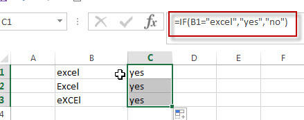
Excel IF function check if a cell contains text(case-insensitive)
By default, IF function is case-insensitive in excel. It means that the logical text for text values will do not recognize case in the IF formulas. For example, the following two IF formulas will get the same results when checking the text values in cells.
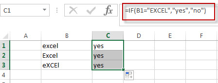
=IF(B1="excel","yes","no")
=IF(B1="EXCEl","yes","no")
The IF formula will check the values of cell B1 if it is equal to “excel” word, If it is TRUE, then return “yes”, otherwise return “no”. And the logical test in the above IF formula will check the text values in the logical_test argument, whatever the logical_test values are “Excel”, “eXcel”, or “EXCEL”, the IF formula don’t care about that if the text values is in lowercase or uppercase, It will get the same results at last.
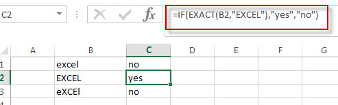
Excel IF function check if a cell contains text (case-sensitive)
If you want to check text values in cells using IF formula in excel (case-sensitive), then you need to create a case-sensitive logical test and then you can use IF function in combination with EXACT function to compare two text values. So if those two text values are exactly the same, then return TRUE. Otherwise return FALSE.
So we can write down the following IF formula combining with EXACT function:
=IF(EXACT(B1,"excel"),"yes","no")
Excel IF function check if part of cell matches specific text
If you want to check if part of text values in cell matches the specific text rather than exact match, to achieve this logic text, you can use IF function in combination with ISNUMBER and SEARCH Function in excel.
Both ISNUMBER and SEARCH functions are case-insensitive in excel.
=IF(ISNUMBER(SEARCH("x",B1)),"good","bad")
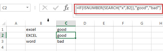
For above the IF formula, it will Check to see if B1 contain the letter x.
Also, we can use FIND function to replace the SEARCH function in the above IF formula. It will return the same results.
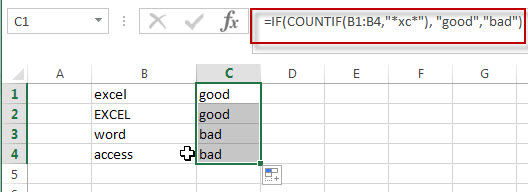
Excel IF function with Wildcards text value
If you wan to use wildcard charcter in an IF formula, for example, if any of the values in column B contains “*xc*”, then return “good”, others return “bad”. You can not directly use the wildcard characters in IF formula, and we can use IF function in combination with COUNTIF function. Let’s see the following IF formula:
=IF(COUNTIF(B1:B4,"*xc*"), "good","bad")
- Excel IF Function With Numbers
If you want to check if a cell values is between two values or checking for the range of numbers or multiple values in cells, at this time, we need to use AND or OR logical function in combination with the logical operator and IF function…
- Excel EXACT function
The Excel SEARCH function returns the number of the starting location of a substring in a text string.The syntax of the EXACT function is as below:= EXACT (text1,text2)… - Excel COUNTIF function
The Excel COUNTIF function will count the number of cells in a range that meet a given criteria.= COUNTIF (range, criteria) … - Excel ISNUMBER function
The Excel ISNUMBER function returns TRUE if the value in a cell is a numeric value, otherwise it will return FALSE. - Excel IF function
The Excel IF function perform a logical test to return one value if the condition is TRUE and return another value if the condition is FALSE…. - Excel SEARCH function
The Excel SEARCH function returns the number of the starting location of a substring in a text string.…
-
05-19-2015, 02:10 AM
#1
Registered User
Weirdest problem ever — excel not matching matching text
I cant explain it really well other than showing an example in file, so I have attached it here.
Basically I downloaded a file with hourly data. I copy pasted it to a new excel document. The index key of the data is two time stamps with the word «to» in between. Like so: [2014-11-18 01:00:00*to 2014-11-18 02:00:00]
For the purpose of what I’m doing, I manually recreated a table with some identical index strings, so I would be able to use LOOKUP to find the value for any of the rows in the original data. Let’s say I wanted the value for the time slot 2014-11-18 01:00:00*to 2014-11-18 02:00:00, I would use a lookup function in the table to get the value corresponding to that timeslot.
The only problem is, even if I type the PERFECT match of the index string into my lookup formula, it still comes out with an #N/A error.
It shouldnt be formatting, because the ‘EXACT’ formula ignores formatting, and still returns FALSE when I try to directly match the index key to my manually entered key. I’m thinking it might be something to do with ASCII/HTML character mismatch or something, but really have run out of ideas how to work it.
/A
-
05-19-2015, 02:12 AM
#2
Registered User
Re: Weirdest problem ever — excel not matching matching text
OK this is even weirder, but after posting I saw that excelforum.com inserted a small * before the word ‘to’. That star was not showing up in excel when I copied the data. If I try to enter a * symbol into the lookup formula EUREKA it works… PLEASE tell me whats going on here!
/A
-
05-19-2015, 03:08 AM
#3
Re: Weirdest problem ever — excel not matching matching text
I copied A2 from the formula bar and pasted it into A6. Your formula works fine. Those strings are not identical. Sometimes non-printable characters will show up in copied data. Try this array formula in E16 and fill down to E17.Array formulas are not committed in the regular way. You commit by pressing and holding Ctrl + Shift as you hit Enter. You will know that it has been entered successfully when you can see curly braces {} around your formula in the formula bar. You do not type these in yourself. Excel does it for you.
It counts character 160. These frequently show up when copying/pasting from tables on the internet. They are non-printable and are difficult to detect. E16 has one E17 does not.
-
05-19-2015, 03:11 AM
#4
Re: Weirdest problem ever — excel not matching matching text
Furhter to Flame retired’s contribution. It is the non-breaking space (Char 160) and you can see exactly where it is here.
-
05-19-2015, 03:15 AM
#5
Re: Weirdest problem ever — excel not matching matching text
-
05-19-2015, 03:26 AM
#6
Re: Weirdest problem ever — excel not matching matching text
I should have added that the formula in brown will substitute an ordinary space (code 32) for any non-breaking spaces (Code 160), allowing the two cells to match exactly.
FlameRetired — enjoy some rest….
-
05-19-2015, 03:33 AM
#7
Registered User
Re: Weirdest problem ever — excel not matching matching text
Hi,
Please refer to Office.com off line help, which quotes as under:
«When searching text values in the first column of table_array, ensure that the data in the first column of table_array does not contain leading spaces, trailing spaces, inconsistent use of straight ( ‘ or » ) and curly ( ‘ or “) quotation marks, or nonprinting characters. In these cases, VLOOKUP might return an incorrect or unexpected value.»
If you remove the spaces, vlookup function executes the result correctly.


![]()
Excel If Cell Contains Text

Excel If Cell Contains Text Then Formula helps you to return the output when a cell have any text or a specific text. You can check if a cell contains a some string or text and produce something in other cell. For Example you can check if a cell A1 contains text ‘example text’ and print Yes or No in Cell B1. Following are the example Formulas to check if Cell contains text then return some thing in a Cell.
If Cell Contains Text
Here are the Excel formulas to check if Cell contains specific text then return something. This will return if there is any string or any text in given Cell. We can use this simple approach to check if a cell contains text, specific text, string, any text using Excel If formula. We can use equals to operator(=) to compare the strings .
If Cell Contains Text Then TRUE
Following is the Excel formula to return True if a Cell contains Specif Text. You can check a cell if there is given string in the Cell and return True or False.
The formula will return true if it found the match, returns False of no match found.
If Cell Contains Partial Text
We can return Text If Cell Contains Partial Text. We use formula or VBA to Check Partial Text in a Cell.
Find for Case Sensitive Match:
We can check if a Cell Contains Partial Text then return something using Excel Formula. Following is a simple example to find the partial text in a given Cell. We can use if your want to make the criteria case sensitive.
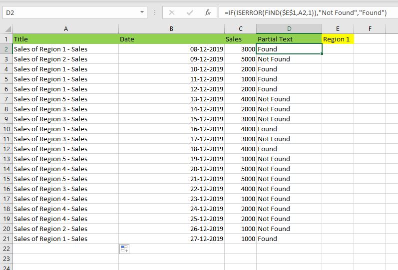
- Here, Find Function returns the finding position of the given string
- Use Find function is Case Sensitive
- IsError Function check if Find Function returns Error, that means, string not found
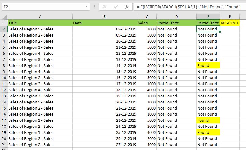
Search for Not Case Sensitive Match:
We can use Search function to check if Cell Contains Partial Text. Search function useful if you want to make the checking criteria Not Case Sensitive.
If Range of Cells Contains Text
We can check for the strings in a range of cells. Here is the formula to find If Range of Cells Contains Text. We can use Count If Formula to check the excel if range of cells contains specific text and return Text.
- CountIf function counts the number of cells with given criteria
- We can use If function to return the required Text
- Formula displays the Text ‘Range Contains Text” if match found
- Returns “Text Not Found in the Given Range” if match not found in the specified range
If Cells Contains Text From List
Below formulas returns text If Cells Contains Text from given List. You can use based on your requirement.
VlookUp to Check If Cell Contains Text from a List:
We can use VlookUp function to match the text in the Given list of Cells. And return the corresponding values.
- Check if a List Contains Text:
=IF(ISERR(VLOOKUP(F1,A1:B21,2,FALSE)),”False:Not Contains”,”True: Text Found”) - Check if a List Contains Text and Return Corresponding Value:
=VLOOKUP(F1,A1:B21,2,FALSE) - Check if a List Contains Partial Text and Return its Value:
=VLOOKUP(“*”&F1&”*”,A1:B21,2,FALSE)
If Cell Contains Text Then Return a Value
We can return some value if cell contains some string. Here is the the the Excel formula to return a value if a Cell contains Text. You can check a cell if there is given string in the Cell and return some string or value in another column.
The formula will return true if it found the match, returns False of no match found. can
Excel if cell contains word then assign value
You can replace any word in the following formula to check if cell contains word then assign value.
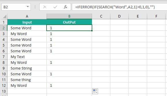
Search function will check for a given word in the required cell and return it’s position. We can use If function to check if the value is greater than 0 and assign a given value (example: 1) in the cell. search function returns #Value if there is no match found in the cell, we can handle this using IFERROR function.
Count If Cell Contains Text
We can check If Cell Contains Text Then COUNT. Here is the Excel formula to Count if a Cell contains Text. You can count the number of cells containing specific text.
The formula will Sum the values in Column B if the cells of Column A contains the given text.
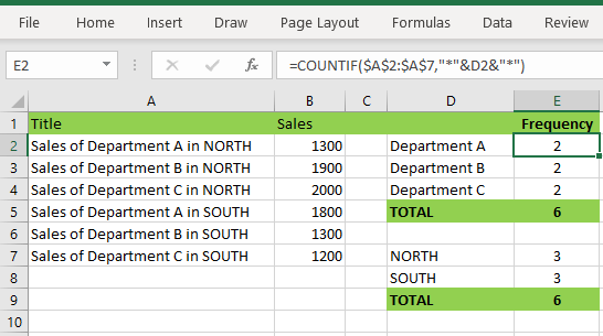
Count If Cell Contains Partial Text
We can count the cells based on partial match criteria. The following Excel formula Counts if a Cell contains Partial Text.
- We can use the CountIf Function to Count the Cells if they contains given String
- Wild-card operators helps to make the CountIf to check for the Partial String
- Put Your Text between two asterisk symbols (*YourText*) to make the criteria to find any where in the given Cell
- Add Asterisk symbol at end of your text (YourText*) to make the criteria to find your text beginning of given Cell
- Place Asterisk symbol at beginning of your text (*YourText) to make the criteria to find your text end of given Cell
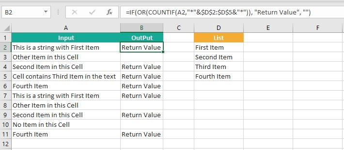
If Cell contains text from list then return value
Here is the Excel Formula to check if cell contains text from list then return value. We can use COUNTIF and OR function to check the array of values in a Cell and return the given Value. Here is the formula to check the list in range D2:D5 and check in Cell A2 and return value in B2.
If Cell Contains Text Then SUM
Following is the Excel formula to Sum if a Cell contains Text. You can total the cell values if there is given string in the Cell. Here is the example to sum the column B values based on the values in another Column.
The formula will Sum the values in Column B if the cells of Column A contains the given text.

Sum If Cell Contains Partial Text
Use SumIfs function to Sum the cells based on partial match criteria. The following Excel formula Sums the Values if a Cell contains Partial Text.
- SUMIFS Function will Sum the Given Sum Range
- We can specify the Criteria Range, and wild-card expression to check for the Partial text
- Put Your Text between two asterisk symbols (*YourText*) to Sum the Cells if the criteria to find any where in the given Cell
- Add Asterisk symbol at end of your text (YourText*) to Sum the Cells if the criteria to find your text beginning of given Cell
- Place Asterisk symbol at beginning of your text (*YourText) to Sum the Cells if criteria to find your text end of given Cell
VBA to check if Cell Contains Text
Here is the VBA function to find If Cells Contains Text using Excel VBA Macros.
If Cell Contains Partial Text VBA
We can use VBA to check if Cell Contains Text and Return Value. Here is the simple VBA code match the partial text. Excel VBA if Cell contains partial text macros helps you to use in your procedures and functions.
MsgBox CheckIfCellContainsPartialText(Cells(2, 1), “Region 1”)
End Sub
Function CheckIfCellContainsPartialText(ByVal cell As Range, ByVal strText As String) As Boolean
If InStr(1, cell.Value, strText) > 0 Then CheckIfCellContainsPartialText = True
End Function
- CheckIfCellContainsPartialText VBA Function returns true if Cell Contains Partial Text
- inStr Function will return the Match Position in the given string
If Cell Contains Text Then VBA MsgBox
Here is the simple VBA code to display message box if cell contains text. We can use inStr Function to search for the given string. And show the required message to the user.
If InStr(1, Cells(2, 1), “Region 3”) > 0 Then blnMatch = True
If blnMatch = True Then MsgBox “Cell Contains Text”
End Sub
- inStr Function will return the Match Position in the given string
- blnMatch is the Boolean variable becomes True when match string
- You can display the message to the user if a Range Contains Text
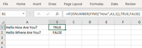
Which function returns true if cell a1 contains text?
You can use the Excel If function and Find function to return TRUE if Cell A1 Contains Text. Here is the formula to return True.
Which function returns true if cell a1 contains text value?
You can use the Excel If function with Find function to return TRUE if a Cell A1 Contains Text Value. Below is the formula to return True based on the text value.
Share This Story, Choose Your Platform!
7 Comments
-
Meghana
December 27, 2019 at 1:42 pm — ReplyHi Sir,Thank you for the great explanation, covers everything and helps use create formulas if cell contains text values.
Many thanks! Meghana!!
-
Max
December 27, 2019 at 4:44 pm — ReplyPerfect! Very Simple and Clear explanation. Thanks!!
-
Mike Song
August 29, 2022 at 2:45 pm — ReplyI tried this exact formula and it did not work.
-
Theresa A Harding
October 18, 2022 at 9:51 pm — Reply -
Marko
November 3, 2022 at 9:21 pm — ReplyHi
Is possible to sum all WA11?
(A1) WA11 4
(A2) AdBlue 1, WA11 223
(A3) AdBlue 3, WA11 32, shift 4
… and everything is in one column.
Thanks you very much for your help.
Sincerely Marko
-
Mike
December 9, 2022 at 9:59 pm — ReplyThank you for the help. The formula =OR(COUNTIF(M40,”*”&Vendors&”*”)) will give “TRUE” when some part of M40 contains a vendor from “Vendors” list. But how do I get Excel to tell which vendor it found in the M40 cell?
-
PNRao
December 18, 2022 at 6:05 am — ReplyPlease describe your question more elaborately.
Thanks!
-
© Copyright 2012 – 2020 | Excelx.com | All Rights Reserved
Page load link
Okay, I have been trying to find a solution for this and I just don’t seem to be able. I can’t even break down the problem properly. This is the idea.
I have two sheets with many rows (one with 800 and the other with 300,000). Each row contains a Name column and then several columns that contain information about this Name. Each sheet has different kinds of information.
I want to consolidate these two sheets into a master sheet based on this Name column they both have, so the consolidate function is perfect for this. Now the problem is that the names don’t match perfectly.
For example Sheet1 contains
«Company B.V.», «Info #1»
«Company Total», «Info #2»
«Company Ltd», «Info #3»
and sheet 2 contains
«Company and Co.», «Info #4»
«Company and Co», «Info #5»
Sheet 1 contains all the names that are going to be used (around a 100 but in different forms as stated above) and sheet 2 contains all these 100 in multiple rows plus names that aren’t in the 100 list and therefore I don’t care about.
How would I make a VBA code project where the end result would be something like this, Master sheet:
«Company», «Info #1», «Info #2», «Info #3», «Info #4», «Info #5»
for every single «Company» (the 100 list) in there??
I do hope there is a solution for this. I’m pretty new to VBA projects, but I have done some minimal coding before.