Text inside cell excel - Word и Excel - помощь в работе с программами

To start a new line of text or add spacing between lines or paragraphs of text in a worksheet cell, press Alt+Enter to insert a line break.

Double-click the cell in which you want to insert a line break.
Click the location inside the selected cell where you want to break the line.
Press Alt+Enter to insert the line break.

To start a new line of text or add spacing between lines or paragraphs of text in a worksheet cell, press CONTROL + OPTION + RETURN to insert a line break.

Double-click the cell in which you want to insert a line break.
Click the location inside the selected cell where you want to break the line.
Press CONTROL+OPTION+RETURN to insert the line break.

To start a new line of text or add spacing between lines or paragraphs of text in a worksheet cell, press Alt+Enter to insert a line break.

Double-click the cell in which you want to insert a line break (or select the cell and then press F2).
Click the location inside the selected cell where you want to break the line.
Press Alt+Enter to insert the line break.

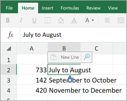
Double-tap within the cell.
Tap the place where you want a line break, and then tap the blue cursor.
Tap New Line in the contextual menu.

Note: You cannot start a new line of text in Excel for iPhone.

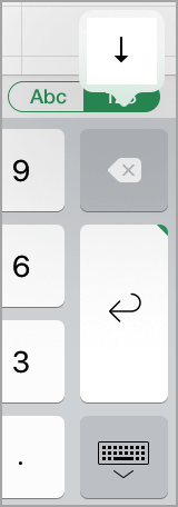
Tap the keyboard toggle button to open the numeric keyboard.
Press and hold the return key to view the line break key, and then drag your finger to that key.

Источник

Содержание

Check if a cell contains text (case-insensitive)
Find cells that contain text
Check if a cell has any text in it
Check if a cell matches specific text
Check if part of a cell matches specific text
Start a new line of text inside a cell in Excel
Need more help?
Start a new line of text inside a cell in Excel
Need more help?
Include text in formulas
Wrap text in a cell
Wrap text automatically
Adjust the row height to make all wrapped text visible
Enter a line break
Need more help?

Check if a cell contains text (case-insensitive)

Let’s say you want to ensure that a column contains text, not numbers. Or, perhapsyou want to find all orders that correspond to a specific salesperson. If you have no concern for upper- or lowercase text, there are several ways to check if a cell contains text.

You can also use a filter to find text. For more information, see Filter data.

Find cells that contain text

Follow these steps to locate cells containing specific text:

Select the range of cells that you want to search.

To search the entire worksheet, click any cell.

On the Home tab, in the Editing group, click Find & Select, and then click Find.

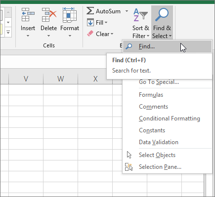
In the Find what box, enter the text—or numbers—that you need to find. Or, choose a recent search from the Find what drop-down box.

Note: You can use wildcard characters in your search criteria.

To specify a format for your search, click Format and make your selections in the Find Format popup window.

Click Options to further define your search. For example, you can search for all of the cells that contain the same kind of data, such as formulas.

In the Within box, you can select Sheet or Workbook to search a worksheet or an entire workbook.

Click Find All or Find Next.

Find All lists every occurrence of the item that you need to find, and allows you to make a cell active by selecting a specific occurrence. You can sort the results of a Find All search by clicking a header.

Note: To cancel a search in progress, press ESC.

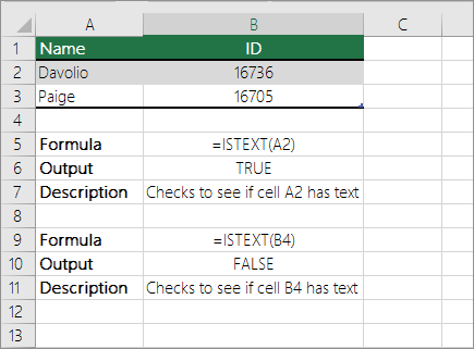
Check if a cell has any text in it

To do this task, use the ISTEXT function.

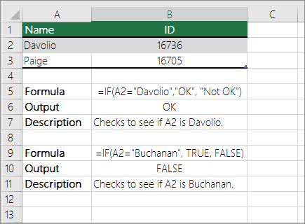
Check if a cell matches specific text

Use the IF function to return results for the condition that you specify.

Check if part of a cell matches specific text

To do this task, use the IF, SEARCH, and ISNUMBER functions.

Note: The SEARCH function is case-insensitive.

Источник

Start a new line of text inside a cell in Excel

To start a new line of text or add spacing between lines or paragraphs of text in a worksheet cell, press Alt+Enter to insert a line break.

Double-click the cell in which you want to insert a line break.

Click the location inside the selected cell where you want to break the line.

Press Alt+Enter to insert the line break.

To start a new line of text or add spacing between lines or paragraphs of text in a worksheet cell, press CONTROL + OPTION + RETURN to insert a line break.

Double-click the cell in which you want to insert a line break.

Click the location inside the selected cell where you want to break the line.

Press CONTROL+OPTION+RETURN to insert the line break.

To start a new line of text or add spacing between lines or paragraphs of text in a worksheet cell, press Alt+Enter to insert a line break.

Double-click the cell in which you want to insert a line break (or select the cell and then press F2).

Click the location inside the selected cell where you want to break the line.

Press Alt+Enter to insert the line break.

Double-tap within the cell.

Tap the place where you want a line break, and then tap the blue cursor.

Tap New Line in the contextual menu.

Note: You cannot start a new line of text in Excel for iPhone.

Tap the keyboard toggle button to open the numeric keyboard.

Press and hold the return key to view the line break key, and then drag your finger to that key.

Need more help?

You can always ask an expert in the Excel Tech Community or get support in the Answers community.

Источник

Start a new line of text inside a cell in Excel

To start a new line of text or add spacing between lines or paragraphs of text in a worksheet cell, press Alt+Enter to insert a line break.

Double-click the cell in which you want to insert a line break.

Click the location inside the selected cell where you want to break the line.

Press Alt+Enter to insert the line break.

To start a new line of text or add spacing between lines or paragraphs of text in a worksheet cell, press CONTROL + OPTION + RETURN to insert a line break.

Double-click the cell in which you want to insert a line break.

Click the location inside the selected cell where you want to break the line.

Press CONTROL+OPTION+RETURN to insert the line break.

To start a new line of text or add spacing between lines or paragraphs of text in a worksheet cell, press Alt+Enter to insert a line break.

Double-click the cell in which you want to insert a line break (or select the cell and then press F2).

Click the location inside the selected cell where you want to break the line.

Press Alt+Enter to insert the line break.

Double-tap within the cell.

Tap the place where you want a line break, and then tap the blue cursor.

Tap New Line in the contextual menu.

Note: You cannot start a new line of text in Excel for iPhone.

Tap the keyboard toggle button to open the numeric keyboard.

Press and hold the return key to view the line break key, and then drag your finger to that key.

Need more help?

You can always ask an expert in the Excel Tech Community or get support in the Answers community.

Источник

Include text in formulas

We often hear that you want to make data easier to understand by including text in your formulas, such as «2,347 units sold.» To include text in your functions and formulas, surround the text with double quotes («»). The quotes tell Excel it’s dealing with text, and by text, we mean any character, including numbers, spaces, and punctuation. Here’s an example:

=A2&» sold «&B2&» units.»

For this example, pretend the cells in column A contain names, and the cells in column B contain sales numbers. The result would be something like: Buchanan sold 234 units.

The formula uses ampersands ( &) to combine the values in columns A and B with the text. Also, notice how the quotes don’t surround cell B2. They enclose the text that comes before and after the cell.

Here’s another example of a common task, adding the date to worksheet. It uses the TEXT and TODAY functions to create a phrase such as «Today is Friday, January 20.»

=»Today is » & TEXT(TODAY(),»dddd, mmmm dd.»)

Let’s see how this one works from the inside out. The TODAY function calculates today’s date, but it displays a number, such as 40679. The TEXT function then converts the number to a readable date by first changing the number to text, and then using «dddd, mmmm dd» to control how the date appears—«Friday, January 20.»

Make sure you surround «ddd, mmmm dd» date format with double quotes, and notice how the format uses commas and spaces. Normally, formulas use commas to separate the arguments—the pieces of data—they need to run. But when you treat commas as text, you can use them whenever you need to.

Finally, the formula uses the & to combine the formatted date with the words «Today is «. And yes, put a space after the «is.»

Источник

Wrap text in a cell

Microsoft Excel can wrap text so it appears on multiple lines in a cell. You can format the cell so the text wraps automatically, or enter a manual line break.

Wrap text automatically

In a worksheet, select the cells that you want to format.

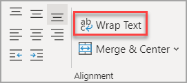
On the Home tab, in the Alignment group, click Wrap Text. (On Excel for desktop, you can also select the cell, and then press Alt + H + W.)

Data in the cell wraps to fit the column width, so if you change the column width, data wrapping adjusts automatically.

If all wrapped text is not visible, it may be because the row is set to a specific height or that the text is in a range of cells that has been merged.

Adjust the row height to make all wrapped text visible

Select the cell or range for which you want to adjust the row height.

On the Home tab, in the Cells group, click Format.

Under Cell Size, do one of the following:

To automatically adjust the row height, click AutoFit Row Height.

To specify a row height, click Row Height, and then type the row height that you want in the Row height box.

Tip: You can also drag the bottom border of the row to the height that shows all wrapped text.

Enter a line break

To start a new line of text at any specific point in a cell:

Double-click the cell in which you want to enter a line break.

Tip: You can also select the cell, and then press F2.

In the cell, click the location where you want to break the line, and press Alt + Enter.

Need more help?

You can always ask an expert in the Excel Tech Community or get support in the Answers community.

Источник

Download Article

If you’re wondering how to create a multiple-line list in a single cell in Microsoft Excel, you’ve come to the right place. Whether you want a cell to contain a bulleted list with line breaks, a numbered list, or a drop-down list, inserting a list is easy once you know where to look. This wikiHow will teach you three helpful ways to insert any type of list to one cell in Excel.

1

Double-click the cell you want to edit. If you want to create a bullet or numerical list in a single cell with each item on its own line, start by double-clicking the cell into which you want to type the list.
2
Insert a bullet point (optional). If you want to preface each list item with a bullet rather than a number or other character, you can use a key shortcut to insert the bullet symbol. Here’s how:
- Mac: Press Option + 8.
- Windows:
  - If you have a numeric keypad on the side of your keyboard, hold down the Alt key while pressing 7 on the keypad.^[1]
  - If not, click the Insert menu, select Symbol, type 2022 into the «Character code» box at the bottom, and then click Insert.
  - If 2022 didn’t bring up a bullet point, select the Wingdings font instead, and then enter 159 as the character code. You can then click Insert to add the bullet point.
Advertisement
3
Type your first list item. Don’t press Enter or Return after typing.
- If you want your list to be numbered, preface the first list item with 1. or 1).
4

Press Alt+↵ Enter (PC) or Control+⌥ Option+⏎ Return on a Mac. This adds a line break so you can start typing on the next line of the same cell.^[2]
5

Type the remaining list items. To continue your list, just enter another bullet point on the second line, type the list item, and press Alt + Enter or Control + Option + Return to open a new line. When you’re finished, you can click anywhere else on your sheet to exit the cell.

1
Create your list in another app. If you’re trying to paste a bullet list (or other type of list) into a single cell rather than have it spread across multiple cells, there’s a trick to pasting the list. Start by creating your list in an app like Word, TextEdit, or Notepad.
- If you create a bulleted list in Word, the bullets will copy over to your cell when pasted into Excel. Bullets may not copy from other apps.
2

Copy the list. To do this, just highlight the list, right-click the highlighted area, and then select Copy.
3

Double-click a cell in Excel. Double-clicking the cell before pasting makes it so the list items will all appear in the same cell.
4

Right-click the cell. The context menu will expand.
5

Click the clipboard icon under «Paste Options.» The icon has a clipboard and a black rectangle. This pastes the list into the cell you double-clicked. Each list item will appear on its own line within the same cell.

1

Open the workbook in which you want to create a drop-down list. If you want to be able to click a cell to view and select from a drop-down list, you can create a list with Excel’s data validation tool.^[3]
2
Create a new worksheet in the workbook. You can do this by clicking the + next to the existing workbook sheets at the bottom of Excel. This worksheet is where you’ll enter the items that you want to appear in your drop-down list.
- After you create the list on a separate sheet and add it to a table, you’ll be able to create a drop-down list containing the list data in any cell you want.
3
Type each list item into a single column. Enter every possible list choice into its own separate cell. The items you type will all be available in the drop-down list.
- If you plan to make a lot of drop-down menus and want to use this same sheet to create all of them, add a header to the top of the list. For example, if you’re making a list of cities, you could type City into the first cell. This header won’t actually appear on the drop-down list you create—it’s just for organization on this sheet that contains list data.
4

Highlight the entire table and press Ctrl+T. Include the header at the top of the list when highlighting. This opens the Create Table dialog.
5
Choose a header option and click OK. If you added a header to the top of your list, check the box next to «My table has headers.» If not, make sure there is no checkmark there before clicking OK.
- Now that your list is in a table, you can make changes to it after creating your drop-down list, and your drop-down list will update automatically.
6

Sort the list alphabetically. This will keep your list organized once you add it to your sheet. To do this, just click the arrow next to your header cell and select Sort A to Z.
7

Click the cell on the worksheet in which you want to add the list. This can be any cell on any worksheet in the workbook.
8

Type a name for the list into the cell. This is the cell where the list will appear, so give it a name that indicates the type of option you should choose from that list. For example, if you made a list of cities, you could type City here.
9

Click the Data tab and select Data Validation. Make sure the cell is selected before doing this. If you don’t see Data Validation in the toolbar, click the icon in the «Data Tools» section that has two black rectangles with a green checkmark and a red circle with a line through it. This opens the Data Validation window.
10

Click the «Allow» menu and select List. Additional options will expand.
11

Click the up-arrow in the «Source» field. This minimizes the Data Validation window so you can select your list data.
12

Select the list (without the header) and press ↵ Enter or ⏎ Return. Click back over to the tab that has your list data and drag the mouse cursor over just the list items. Pressing Enter or Return will add the range to the «Source» field.
13

Click OK. The selected cell now has a drop-down list. If you need to add or remove items from the list, you can simply make those changes on your new worksheet and they’ll automatically propagate to the list.

Ask a Question

200 characters left

Include your email address to get a message when this question is answered.

Submit

Thanks for submitting a tip for review!

About This Article

Article SummaryX

1. Double-click the cell.
2. Press Alt + 7 or Option + 8 to add a bullet point.
3. Type a list item.
4. Press Alt + Enter (PC) or Control + Option + Return (Mac) to go to the next line.
5. Repeat until your list is finished.

Did this summary help you?

Thanks to all authors for creating a page that has been read 62,222 times.

Is this article up to date?

Источник

A normal Excel sheet has cells that are 8.43 points in width and 15 points in height. This is usually about 64 pixels wide and 20 pixels tall.

If your text data is long, you can increase the cell width to fit the data length.

A better option might be to wrap the text to increase the row height so the data fits in the cell instead!

In this post you’ll learn 3 ways to wrap your text data to fit it inside the cell.

What is Text Wrap?

This means that if text is too long to fit inside its cell, it will automatically adjust to appear on multiple lines within the cell.

The data inside the cell will not change and no line break characters will be inserted. It will only appear to be formatted on multiple lines.

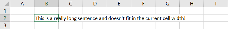
The above example you can see the text inside cell B2 extends well past the width of the cell and spills over cell to the right.

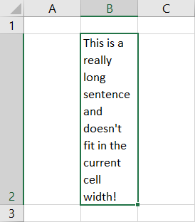
After the cell has had wrap text applied, you can see the row height has been adjusted to fit all the text.

Wrap Text from Ribbon

This is a very common action, so it can be found in the Home tab of the ribbon commands.

Wrap your text.

Select the cell or range of cells to which you want to apply the wrap text formatting.
Go to the Home tab.
Press the Wrap Text command found in the Alignment section.

This will apply the formatting to your cells!

It’s a good idea to adjust the width of your cells to the desired size first as the height of the rows will be adjusted so all the text fits inside the cell.

Wrap Text Keyboard Shortcut

There is no dedicated keyboard shortcut for the wrap text formatting, but you can still use the Alt hotkeys for this.

Select the cells to which you want to apply wrap text then press Alt ➜ H ➜ W.

Certainly a quick and easy way to apply the formatting.

Wrap Text in the Format Cells Dialog Box

The format cells dialog box contains all the formatting options you can apply to a cell in your spreadsheet, including the wrap text option.

You can open this menu with a right click on the cells then choose Format Cells or by using the Ctrl + 1 keyboard shortcut.

Go to the Alignment tab in the menu ➜ Check the Wrap text option in the Text control section ➜ then press the OK button.

This is a great option when you want to apply wrap text and other formatting options at the same time.

Automatically Adjust Row Height to Fit Text

If your row height does not properly adjust to fit all the text and is either too small or too big, then you will need to adjust it.

You can do this manually by clicking and dragging the row but there is an easy option to auto-adjust the height.

Go to the Home tab ➜ select the Format options ➜ then select AutoFit Row Height from the menu. You can also do this by double clicking on the edge of the row heading.

The row height will adjust to the exact height needed to show all the text.

Manually Add Line Breaks to Wrap Your Text

The wrap text option will automatically format your text with line breaks based on the available width of the cell.

If you want to choose where the line breaks appear, then you can do this by manually adding line break characters to your text data.

Place the cursor in the text at the point where you want to add a line break then hold the Alt key and press Enter.

This will add a line break character into your text data and the data will appear on multiple lines in the sheet.

Remove Wrap Text

It’s just as easy to remove wrap text formatting as it is to apply it in the first place.

Remove Formatting

Select the cells from which you want to remove the formatting and then perform any of these methods.

Go to the Home tab and press the Wrap Text command.
Open the Format Cells menu and uncheck the Wrap text option in the Alignment tab.
Use the Alt ➜ H ➜ W keyboard shortcut.

The exact same commands used to apply the formatting can be used to remove the formatting as well!

Remove Manually Added Line Breaks

If you’ve manually added line break characters to your text to achieve a wrapping effect, then you will need to remove them using a find and replace method.

Press Ctrl + H to open the find and replace dialog box.

Place the cursor in the Find what section and press Ctrl + J to add a line break character. Leave the Replace with section empty and then press the Replace All button.

This will replace all the line break character that you manually added by nothing thereby removing them.

Conclusions

Wrapping text is a great option for styling your spreadsheets and making them more readable.

It’s great too, because it’s very easy to do.

What’s your favourite method? Let me know in the comments!

About the Author

John MacDougall

John is a Microsoft MVP and qualified actuary with over 15 years of experience. He has worked in a variety of industries, including insurance, ad tech, and most recently Power Platform consulting. He is a keen problem solver and has a passion for using technology to make businesses more efficient.

Источник

This post will guide you how to insert character or text in middle of cells in Excel. How do I add text string or character to each cell of a column or range with a formula in Excel. How to add text to the beginning of all selected cells in Excel. How to add character after the first character of cells in Excel.

Assuming that you have a list of data in range B1:B5 that contain string values and you want to add one character “E” after the first character of string in Cells. You can refer to the following two methods.

Table of Contents

1. Insert Character or Text to Cells with a Formula
2. Insert Character or Text to Cells with VBA
3. Video: Insert Character or Text to Cells
4. Related Functions

1. Insert Character or Text to Cells with a Formula

To insert the character to cells in Excel, you can use a formula based on the LEFT function and the MID function. Like this:

=LEFT(B1,1) & "E" & MID(B1,2,299)

Type this formula into a blank cell, such as: Cell C1, and press Enter key. And then drag the AutoFill Handle down to other cells to apply this formula.

insert text to cells1

This formula will inert the character “E” after the first character of string in Cells. And if you want to insert the character or text string after the second or third or N position of the string in Cells, you just need to replace the number 1 in Left function and the number 2 in MID function as 2 and 3. Like below:

=LEFT(B1,2) & "E" & MID(B1,3,299)

insert text to cells2

You can also use an Excel VBA Macro to insert one character or text after the first position of the text string in Cells. Just do the following steps:

Step1: open your excel workbook and then click on “Visual Basic” command under DEVELOPER Tab, or just press “ALT+F11” shortcut.

Step2: then the “Visual Basic Editor” window will appear.

Step3: click “Insert” ->”Module” to create a new module.

Step4: paste the below VBA code into the code window. Then clicking “Save” button.

insert text to cells3

Sub AddCharToCells()
    Dim cel As Range
    Dim curR As Range
    Set curR = Application.Selection
    Set curR = Application.InputBox("select one Range that you want to insert one 
    character", "add character to cells", curR.Address, Type: = 8)
    For Each cel In curR
        cel.Value = VBA.Left(cel.Value, 1) & "E" & VBA.Mid(cel.Value, 2, 
        VBA.Len(cel.Value) - 1)
    Next
End Sub

Step5: back to the current worksheet, then run the above excel macro. Click Run button.

insert text to cells4

Step6: select one Range that you want to insert one character.
insert text to cells5

Step7: lets see the result.

insert text to cells6

3. Video: Insert Character or Text to Cells

This video will demonstrate how to insert character or text in middle of cells in Excel using both formulas and VBA code.

Excel MID function
The Excel MID function returns a substring from a text string at the position that you specify.The syntax of the MID function is as below:= MID (text, start_num, num_chars)…
Excel LEFT function
The Excel LEFT function returns a substring (a specified number of the characters) from a text string, starting from the leftmost character.The LEFT function is a build-in function in Microsoft Excel and it is categorized as a Text Function.The syntax of the LEFT function is as below:= LEFT(text,[num_chars])…

Источник

Hi Oz and welcome to the forum,

With Sheet2 as shown in your example, perhaps try this formula in C1 of Sheet1 (I have amended some of the values to better represent the results). Adjust the ranges as appropriate and drag down the formula as far as required:

Sheet1

	A	B	C
1	p6769705	Lot# * 2-3182 ID lot 50643000	11
2	p6769756	* 2-3186 LOT 50642917	14
3	p6769758	3221545	11

Excel 2010

Worksheet Formulas

Cell	Formula
C1	=LOOKUP(2, 1/SEARCH(Sheet2!A$1:A$3,B1), Sheet2!B$1:B$3)

Note:

This formula setup is explained in great detail by Aladin Akyurek here: http://www.mrexcel.com/forum/excel-questions/99621-lookup-value-unsorted-data.html#post492425
The only slight difference being the SEARCH function used in the lookup_vector argument. Here is a concise explanation of how SEARCH works: MS Excel: SEARCH Function (WS)
Since you mentioned you are new to Excel, the following notes on range referencing may also be of use:
- Office 2010 Class #25: Excel Cell References: Relative, Absolute, Mixed — YouTube
- Switch between relative, absolute, and mixed references — Excel — Office.com
- Relative And Absolute Range References

Last edited: Nov 22, 2012

This is Magic!!! thanks Circled for the great help, one day I will be a master like you! Nice links, they explain everything in detail there but I’m less familiar to excel concepts plus my english is not perfect so to understand them I will take some classes before Christmas…

Last edited: Nov 23, 2012

This is Magic!!! thanks Circled for the great help, one day I will be a master like you! Nice links, they explain everything in detail there but I’m less familiar to excel concepts plus my english is not perfect so to understand them I will take some classes before Christmas…

You’re welcome — thanks for the feedback! (I’m no master haha — but I hope you will be one day!)

…

Worksheet Formulas

Cell Formula

C1 =LOOKUP(2, 1/SEARCH(Sheet2!A$1:A$3,B1), Sheet2!B$1:B$3)

<tbody>

</tbody>

<tbody>

</tbody>

[…]

We could avoid the division though…

=LOOKUP(9.99999999999999E+307,SEARCH(Sheet2!A$1:A$3,B1),Sheet2!B$1:B$3)

We could avoid the division though…

=LOOKUP(9.99999999999999E+307,SEARCH(Sheet2!A$1:A$3,B1),Sheet2!B$1:B$3)

Aladin, on the other hand, is a master

You guys are Great!, Aladin, thanks for your time and for spreading the knowledge with us. Do you want to read something funny? I’m the most experienced excel user in my company… (LOL), so i will be be posting some more questions, for sure i’m struggling 3 or 4 days with something before asking guys , with this help in this thread you save me like 8 hours of so manual work with Excel (I know what i’m talking about since i did it with a previous file). Conclusion, is great to have you here Circled/Aladin!

We could avoid the division though…

=LOOKUP(9.99999999999999E+307,SEARCH(Sheet2!A$1:A$3,B1),Sheet2!B$1:B$3)

We can also avoid that real long number…

=LOOKUP(32768,SEARCH(Sheet2!A$1:A$3,B1),Sheet2!B$1:B$3)

You guys are Great!, Aladin, thanks for your time and for spreading the knowledge with us. Do you want to read something funny? I’m the most experienced excel user in my company… (LOL), so i will be be posting some more questions, for sure i’m struggling 3 or 4 days with something before asking guys , with this help in this thread you save me like 8 hours of so manual work with Excel (I know what i’m talking about since i did it with a previous file). Conclusion, is great to have you here Circled/Aladin!

Thanks Oz! I’m glad it saved you some time.

We can also avoid that real long number…

=LOOKUP(32768,SEARCH(Sheet2!A$1:A$3,B1),Sheet2!B$1:B$3)

T. Valko — also a master!

I’ve seen a few threads where you and Aladin discuss 9.99999999999999E+307. Personally, I prefer using the long number and think it is a reasonable choice as a convention for this class of formulae.

I think it helps to keep to a convention for these types of problems and the benefits outweigh the perceived ‘ugliness’. It helps with maintainability and understandability in the long-term over, for example, arbitrarily large numbers that suit each situation which can conceal the underlying intent. Sticking to it as a standard may also mean people who see this type of formulae for the first time can find help a little more easily.

That’s just my view, for now at least — and not that either of you care or should care about it! :LOL:

If anyone is interested, there is an article by Douglas Crockford that is very loosely related to this topic but talks a little bit about why programming (JavaScript) style is important. The first few general paragraphs are maybe somewhat applicable here:
The Elements of JavaScript Style

Last edited: Nov 25, 2012

Thanks Oz! I’m glad it saved you some time.

T. Valko — also a master!

I’ve seen a few threads where you and Aladin discuss 9.99999999999999E+307. Personally, I prefer using the long number and think it is a reasonable choice as a convention for this class of formulae.

I think it helps to keep to a convention for these types of problems and the benefits outweigh the perceived ‘ugliness’. It helps with maintainability and understandability in the long-term over, for example, arbitrarily large numbers that suit each situation which can conceal the underlying intent. Sticking to it as a standard may also mean people who see this type of formulae for the first time can find help a little more easily.

That’s just my view, for now at least — and not that either of you care or should care about it!

If anyone is interested, there is an article by Douglas Crockford that is very loosely related to this topic but talks a little bit about why programming (JavaScript) style is important. The first few general paragraphs are maybe somewhat applicable here:
The Elements of JavaScript Style

I prefer to keep things simple!

Источник

It’s gotta be in here somewhere …

Update: Based on questions I’ve received, I added the Misc Notes section to the end of this post.

Continuing with our #FunctionFriday series, today we’re going to explore how to use the IF, SEARCH, and ISNUMBER functions together to find text (aka a string) inside other text for classification purpose. What Excel really needs is a CONTAINS function, so we don’t have to do these mental acrobats. But, for now, this is what we have to work with.

To illustrate it, I’ll use an example from a chart I include in client dashboards** where they use the AddThis or ShareThis WordPress plugin. The data from these plugins populates to your Google Analytics account. BUT the data is such a red-hot mess, you have to do some cleanup to get it all into nice, neat buckets.

If you’d like to include this report in your own reports, you can use this custom report I created. (If you get a 404 error, it’s because you’re not logged in to Google Analytics. You have to be logged in to apply the report to your Google Analytics profile, aka view.)

**If you want to become a beast at building dashboards using the Google Analytics API, my online course will take you there.

Download Excel Workbook

If you’d like to follow along, you can download the Excel workbook I used in this demo.

The Functions du Jour

IF Function

The IF function is the Swiss Army knife for marketers, especially when you’re building out dynamic dashboards. With the IF function you start with a test — e.g., if A3=B2, if A3>=100, if A3=”organic”, etc. — and then you specify what you want to return if the condition is true and what you want to return if the value is false. But the fun doesn’t stop there; you can actually embed IF functions inside of IF functions. And that’s what we’re going to do in this tutorial.

It follows the following syntax:

IF(logical_test, [value_if_true], [value_if_false])

SEARCH Function

The SEARCH function is a tricky little bugger. It returns the position of whatever character you search for. And if you enter a string of characters, it will return the position of the first character in the matching string. So if you searched for cheese in the string string cheese, it would return the value of 8.

The SEARCH function follows the following syntax:

SEARCH( substring, string, [start_position] )

substring: Pure, unbridled geek speak that means whatever text you’re searching for, e.g., cheese.

string: Typically the cell this text string is in, though you could enter text as long as you flank it with quotation marks. (I almost always use a cell reference.)

start_position: This is optional. I usually only use it when I’m searching for forward slashes in URLs and want to start searching after the http(s)://. You can check out an example in this post that describes how to extract domains from URLs.

Now, if you put a string inside a SEARCH function, it will look for that string exactly. But you can also throw the asterisk wildcard in there for a really good time, which tells Excel to flag any string that even contains the text you’re searching for. So going back to our string cheese example, if I searched for cheese, it would return FALSE; if I searched for *cheese*, it would return TRUE.

ISNUMBER Function

The ISNUMBER function simply tells you if the cell you’re referencing is a value (or number). It’s Boolean, meaning it returns either a value of TRUE or FALSE.

It follows the following syntax:

ISNUMBER(value)

Pro Tip

When dealing with a more complicated IF function, like you’ll see below, a good strategy is to break it into separate lines in the formula bar. To add a line break on a PC, use Alt-Enter; on a Mac, use Control-Option-Enter. I break my IF functions into different lines if I have more than three nested IFs. Here’s what it looks like for the formula we’ll use:

Click for larger image

If you fat finger something in your formula, it’s really easy to see using this strategy because the IF functions won’t line up. When I’m finished, I just collapse the formula bar back to size by clicking-and-dragging the bottom of it.

Here’s what that same formula would look like if I didn’t use line breaks:

Click for larger image

Putting It All Together

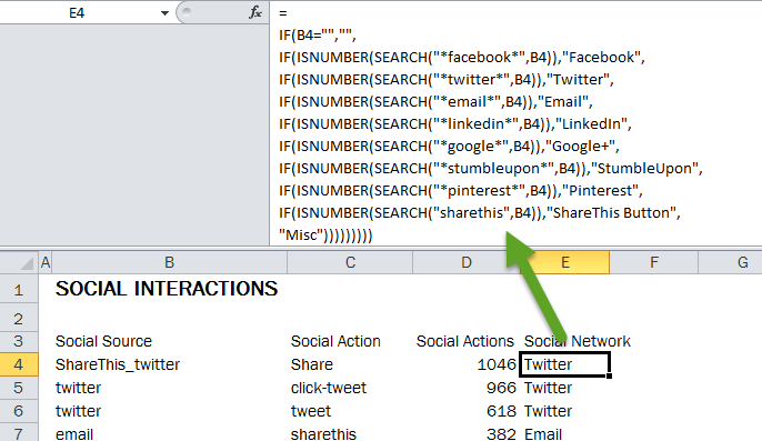
Okay, so here’s how we’re going to use them in concert. The Google Analytics custom report we’re using in this demo uses two dimensions: Social Source and Social Action and one metric, Social Actions. It’s a flat report, which, betedubs, is perfect for pivot tables. (Again, you should have data in this report if you use the ShareThis or AddThis plugin on WordPress.) But you could use this same strategy with any marketing data that you have to bucket based on snippets of text inside of strings.

If the formula in cell E4 could talk in plain English (wouldn’t that be nice?), here’s what it would say: “Hey, Excel, check out cell B4. If you see the string facebook anywhere in there, ISNUMBER will return a value of TRUE because you’ll return a number telling me the position of where the string I’m searching for. I don’t actually care about where that string is, only that it returns a number. If it does (IOW, it returns a value of TRUE), return the string Facebook; if it’s false, look for the next sting (i.e., twitter) and return Twitter … Rinse and repeat until you’ve cycled through all of the criteria. And if you don’t find facebook, twitter, email, linkedin, google, stumbleupon, pinterest, or sharethis, just call it Misc.” (Obviously, switch out sharethis for addthis if you’re using that plugin.)

Misc Notes

Difference Between SEARCH and FIND

Someone asked me about using the FIND function on Facebook instead of SEARCH. I rarely use the FIND function because it’s not as flexible as SEARCH. For one, it’s case sensitive. I can only remember one time using it because I needed to differentiate between cases. A much bigger liability is you can’t use it for partial matches because it doesn’t support Excel’s wildcard characters (* and ?).

Extracting Text Instead Of Categorizing It

So what if you didn’t want to match exact or partial text for the purpose of categorizing it like I have in this post with the help of the IF and ISNUMBER functions? What if, instead, you wanted to extract it instead? Then you would use the SEARCH function with the LEFT, RIGHT, and/or MID functions. I demonstrate how to do that in this tutorial on pulling domain names from a list of URLs. (I use this technique in conjunction with pivot tables in just about all competitive analysis I do because it allows me to group backlinks by domain.)

Image credit

~~~

If you would like to learn more about Excel, check out my Excel dashboard course. 24 instructional videos, totaling 6+ hours of instruction for $95.

Источник

01-29-2005, 07:06 PM

#1

How do I create a bulleted list text format inside cell?

I am collecting data and want to format the text inside the «notes» (my
title) cell so that it can be more easily read. I would like to make a
bulleted list. There are several cells that need this formatting. Is this
possible?
01-29-2005, 07:06 PM

#2

Re: How do I create a bulleted list text format inside cell?

There is no help for this. You have to do it manually.

—
Regards,
Tom Ogilvy

«DEH» <DEH@discussions.microsoft.com> wrote in message
news:DFAEE5CC-0AAD-41D7-9DE1-396187DA2681@microsoft.com…

> I am collecting data and want to format the text inside the «notes» (my
> title) cell so that it can be more easily read. I would like to make a
> bulleted list. There are several cells that need this formatting. Is this
> possible?
01-30-2005, 05:06 PM

#3

RE: How do I create a bulleted list text format inside cell?

Thank you for the help. Is there a way to atleast list the items line by line
in the same cell…That is, «press return» without leaving the cell?

«DEH» wrote:

> I am collecting data and want to format the text inside the «notes» (my
> title) cell so that it can be more easily read. I would like to make a
> bulleted list. There are several cells that need this formatting. Is this
> possible?
01-30-2005, 06:06 PM

#4

Re: How do I create a bulleted list text format inside cell?

Use alt-enter to force a new line within the cell.

As a formula:

=a1&char(10)&»hi there»&char(10)&b1

You may have to turn on wrap text (if you see square boxes where those
alt-enters are).
format|cells|alignment tab

DEH wrote:

>
> Thank you for the help. Is there a way to atleast list the items line by line
> in the same cell…That is, «press return» without leaving the cell?
>
> «DEH» wrote:
>
> > I am collecting data and want to format the text inside the «notes» (my
> > title) cell so that it can be more easily read. I would like to make a
> > bulleted list. There are several cells that need this formatting. Is this
> > possible?

—

Dave Peterson
01-31-2005, 02:06 AM

#5

Re: How do I create a bulleted list text format inside cell?

In a cell hit ALT + 0149(from NumPad)

Type some text then hit ALT + ENTER.

Hit ALT + 0149 then type some more text.

The ALT + ENTER will give a carriage return.

The ALT + 0149 will give a Bullet.

Gord Dibben Excel MVP

On Sun, 30 Jan 2005 12:47:01 -0800, DEH <DEH@discussions.microsoft.com> wrote:

>Thank you for the help. Is there a way to atleast list the items line by line
>in the same cell…That is, «press return» without leaving the cell?
>
>»DEH» wrote:
>
>> I am collecting data and want to format the text inside the «notes» (my
>> title) cell so that it can be more easily read. I would like to make a
>> bulleted list. There are several cells that need this formatting. Is this
>> possible?
02-01-2005, 04:06 AM

#6

Re: How do I create a bulleted list text format inside cell?

Thank you…big help!
Sincerely,
Debbie Hope

«Dave Peterson» wrote:

> Use alt-enter to force a new line within the cell.
>
> As a formula:
>
> =a1&char(10)&»hi there»&char(10)&b1
>
> You may have to turn on wrap text (if you see square boxes where those
> alt-enters are).
> format|cells|alignment tab
>
> DEH wrote:
> >
> > Thank you for the help. Is there a way to atleast list the items line by line
> > in the same cell…That is, «press return» without leaving the cell?
> >
> > «DEH» wrote:
> >
> > > I am collecting data and want to format the text inside the «notes» (my
> > > title) cell so that it can be more easily read. I would like to make a
> > > bulleted list. There are several cells that need this formatting. Is this
> > > possible?
>
> —
>
> Dave Peterson
>

Источник

Check if a cell contains text (case-insensitive)

Find cells that contain text

Check if a cell has any text in it

Check if a cell matches specific text

Check if part of a cell matches specific text

Start a new line of text inside a cell in Excel

Need more help?

Start a new line of text inside a cell in Excel

Need more help?

Include text in formulas

Wrap text in a cell

Wrap text automatically

Adjust the row height to make all wrapped text visible

Enter a line break

Need more help?

About This Article

Is this article up to date?

What is Text Wrap?

Wrap Text from Ribbon

Wrap Text Keyboard Shortcut

Wrap Text in the Format Cells Dialog Box

Automatically Adjust Row Height to Fit Text

Manually Add Line Breaks to Wrap Your Text

Remove Wrap Text

Remove Formatting

Remove Manually Added Line Breaks

Conclusions

About the Author

1. Insert Character or Text to Cells with a Formula

3. Video: Insert Character or Text to Cells

Download Excel Workbook

The Functions du Jour

IF Function

SEARCH Function

ISNUMBER Function

Pro Tip

Putting It All Together

Misc Notes

Difference Between SEARCH and FIND

Extracting Text Instead Of Categorizing It

How do I create a bulleted list text format inside cell?

Re: How do I create a bulleted list text format inside cell?

RE: How do I create a bulleted list text format inside cell?

Re: How do I create a bulleted list text format inside cell?

Re: How do I create a bulleted list text format inside cell?

Re: How do I create a bulleted list text format inside cell?