Тест дики фуллера excel

We consider the stochastic process of form

where |φ| ≤ 1 and ε_i is white noise. If |φ| = 1, we have what is called a unit root. In particular, if φ = 1, we have a random walk (without drift), which is not stationary. In fact, if |φ| = 1, the process is not stationary, while if |φ| < 1, the process is stationary. We won’t consider the case where |φ| > 1 further since in this case the process is called explosive and increases over time.

This process is a first-order autoregressive process, AR(1), which we study in more detail in Autoregressive Processes. We will also see why such processes without a unit root are stationary and why the term “root” is used.

The Dickey-Fuller test is a way to determine whether the above process has a unit root. The approach used is quite straightforward. First calculate the first difference, i.e.

i.e.

If we use the delta operator, defined by Δy_i = y_i – y_i-1 and set β = φ – 1, then the equation becomes the linear regression equation

where β ≤ 0 and so the test for φ is transformed into a test that the slope parameter β = 0. Thus, we have a one-tailed test (since β can’t be positive) where

H₀: β = 0 (equivalent to φ = 1)

H₁: β < 0 (equivalent to φ < 1)

Under the alternative hypothesis, if b is the ordinary least squares (OLS) estimate of β, and so φ-bar = 1 + b is the OLS estimate of φ, then for large enough n

where

We can use the usual linear regression approach, except that when the null hypothesis holds the t coefficient doesn’t follow a normal distribution and so we can’t use the usual t-test. Instead, this coefficient follows a tau distribution, and so our test consists of determining whether the tau statistic τ (which is equivalent to the usual t statistic) is less than τ_crit based on a table of critical tau statistics values shown in Dickey-Fuller Table.

If the calculated tau value is less than the critical value in the table of critical values, then we have a significant result; otherwise, we accept the null hypothesis that there is a unit root and the time series is not stationary.

There are the following three versions of the Dickey-Fuller test:

Type 0	No constant, no trend	Δyi = β1 yi-1 + εi
Type 1	Constant, no trend	Δyi = β0 + β1 yi-1 + εi
Type 2	Constant and trend	Δyi = β0 + β1 yi-1 + β2 i+ εi

Each version of the test uses a different set of critical values, as shown in the Dickey-Fuller Table. It is important to select the correct version of the test for the time series being analyzed. Note that the type 2 test assumes there is a constant term (which may be significantly equal to zero).

Example 1: The net daily earnings of a small-time gambler are listed in column B of Figure 1. Use the Dickey-Fuller test to determine whether the times series is stationary.

We start by assuming that the correct model is type 1, namely constant but no trend.

Figure 1 – Regression on time-series data

Since we are using the regression model

(constant, no trend) we use the Real Statistics Linear Regression data analysis tool using range B4:B27 and the X data range and D5:D28 as the Y data range. Note that the values in column D are calculated by placing the formula =B5-B4 in cell D5, highlighting the range D5:D28 and pressing Ctrl-D.

The output from the regression analysis is shown on the right side of Figure 1. In particular, we see that the t statistic (cell I20) for the β₁ coefficient is -1.91613. This is the tau statistic. We now look up in the Dickey-Fuller Table, and find that the tau critical value for a type 1 test is -2.986 when n = 25 and α = .05. Since τ_crit = -2.986 < – 1.91613 = τ, we cannot reject the null hypothesis that the time series is not stationary.

Note that the β₁ coefficient (cell G20) is negative as expected. If instead, the coefficient were positive, then we would know that this type of Dickey-Fuller test was inappropriate since β₁ = φ – 1 ≤ 0.

We now display in Figure 2 a plot of the time series values from Figure 1.

Figure 2 – Chart of Winnings by Day

We see that there is an apparent downward trend towards the end of the 25 day period and so it is not surprising that the time series is not stationary. In fact, this leads us to choose the type 2 Dickey-Fuller test (with constant and trend). The result of this test is shown in Figure 3.

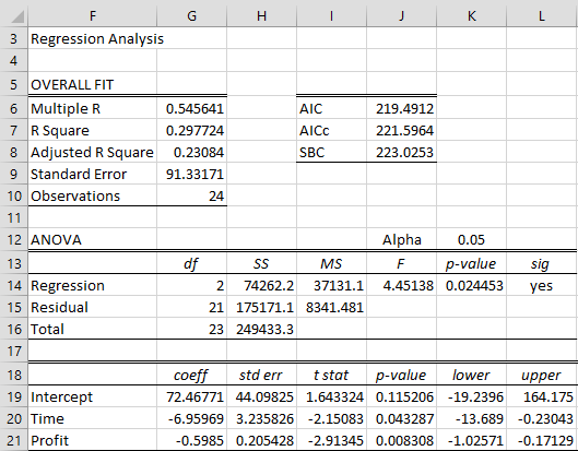
Figure 3 – Dickey-Fuller with trend

Since we are using the regression model

Δy_i = β₀ + β₁i + β₂y_i-1 + ε_i

this time, we use A4:B27 from Figure 1 as the X data range and D5:D28 as the Y data range. We see from Figure 3 that the t statistic (cell I21) for the β₂ coefficient is -2.91345. We now look up in the Dickey-Fuller Table, and find that the tau critical value is -3.60269 for a type 2 test when n = 25 and α = .05. Since τ_crit = -3.60269 < -2.91345 = τ, we cannot reject the null hypothesis that the time series is not stationary.

Real Statistics Function: The Real Statistics Resource Pack provides the following array function where R1 contains a column of time series data.

ADFTEST(R1, lab, , , type, alpha): returns a 3 × 1 range which contains the following values: tau-statistic, tau-critical, yes/no (stationary or not)

If lab = TRUE (default is FALSE), the output consists of a 3 × 2 range whose first column contains labels. type = the test type (0, 1, 2, default is 1). The default value for alpha is .05.

Note that for the type 2 test for Example 1, the output from the array formula

=ADFTEST(R6:R30,TRUE,,,2,U9)

agrees with the results we obtained above, as displayed in Figure 4.

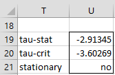
Figure 4 – Output from ADFTEST function

Note that the ADFTEST function can also be used to conduct the Augmented Dickey-Fuller test (ADF). See Augmented Dickey-Fuller Test. In fact, the ADFTEST function can take additional arguments and output other values, as explained on that webpage.

Real Statistics Function: The Real Statistics Resource Pack provides the following functions

ADFCRIT(n, alpha, type) = critical value, tau-crit, for the stated type of ADF test at the stated alpha value, when the time series has n elements

ADFPROB(x, n, type) = estimated p-value (based on linear interpolation) for the ADF test at x

Thus for Example 1, we see that ADFCRIT(25,.05,2) = -3.60269.

Thus for Example 1, ADFCRIT(25,.05,2) = -3.60269. Also, ADFPROB(-2.91345,25,2) = “>.1”. ADFPROB takes values between .01 and .10; values greater than .1 are output as “>.1” and values less than .01 are output as “<.01”. Note that in the constant without trend case, if the tau-stat were -2.91345, then p-value = ADFPROB(-2.91345,25,1) = .060127.

Note that the ADFCRIT function will return critical values for alpha = .01, .025, .05 and .10 and for values of n found in the Dickey-Fuller Table as well as for values of alpha and n not included in the table.

Тест ADF (расширенный тест Дики – Фуллера) – проверка Статистической значимости (Statistical Significance), которая демонстрирует результаты проверки Нулевой гипотезы (Null Hypothesis) и Альтернативной (Alternative Hypothesis). В результате мы получим P-значение (P Value), из которого можно сделать вывод о Стационарности (Stationarity) Временного ряда (Time Series). Был предложен в 1979 году Дэвидом Дики и Уэйном Фуллером.

Когда мы создаем прогнозирующую Модель (Model) для временных рядов, нам требуются стационарные временные ряды, то есть обладающие одинаковой Ковариацией (Covariance) Выборок (Sample) одного размера. Ковариация – мера взаимосвязи двух случайных величин, измеряющая общее отклонение двух случайных величин от их ожидаемых значений. Метрика оценивает, в какой степени переменные изменяются вместе. Другими словами, это мера Дисперсии (Variance) между двумя переменными.

Тестирование на стационарность часто используется в Авторегрессионном моделях (Autoregressive Model). Мы можем выполнять различные тесты, такие как Критерий KPSS, Тест Филлипса – Перрона (Phillips-Perron Test) и ADF – тема этой статьи. Мы рассмотрим логику, стоящую за тестом, и реализуем ее с помощью временного ряда.

Мы проведем ADF-тест с нестационарными данными о пассажирах авиакомпаний и стационарными данными о температуре.

ADF: statsmodels

Для начала импортируем необходимые библиотеки:

from statsmodels.tsa.stattools import adfuller
import pandas as pd
import numpy as np

Нестационарный временной ряд

Мы будем использовать Датасет (Dataset) о числе пассажиров одной авиакомпании:

path = ‘https://www.dropbox.com/s/cdjjafehpd0tmbw/AirPassengers.csv?dl=1’
data = pd.read_csv(path)
data.plot(figsize = (14, 8), title = ‘Число пассажиров’)

Теперь, когда у нас есть все, что нужно, мы можем выполнить ADF-тест:

result = adfuller(data[‘#Passengers’], autolag=’AIC’)

print(‘Критерий ADF: %f’ % result[0])

print(‘P-значение: %f’ % result[1])

print(‘Критические значения:’)

for key, value in result[4].items():
print(‘t%s: %.3f’ % (key, value))
if result[0] < result[4][«5%»]:
print («Нулевая гипотеза отвергнута – Временной ряд стационарен»)
else:
print («Нулевая гипотеза не отвергнута – Временной ряд не стационарен»)

Вот такие мы получим метрики:

Критерий ADF: 0.815369
P-значение: 0.991880
Критические значения:
1%: -3.482
5%: -2.884
10%: -2.579
Нулевая гипотеза не отвергнута – Временной ряд не стационарен

P-значение для временного ряда больше 5%, и, соответственно, нулевая гипотеза не отвергнута, а временной ряд нестационарен.

Стационарный временной ряд

Загрузим данные о температуре в Австралии:

path = ‘https://www.dropbox.com/s/i8xs9myposohyp9/temperature.csv?dl=1’
data = pd.read_csv(path)
data.plot(figsize = (14, 8), title = ‘Температура’)

Это средние значения температуры за день в течение нескольких лет:

Проверим этот временной ряд на стационарность:

result = adfuller(data[‘Temp’], autolag = ‘AIC’)

print(‘Критерий ADF: %f’ % result[0])

print(‘P-значение: %f’ % result[1])

print(‘Критические значения:’)

for key, value in result[4].items():
print(‘t%s: %.3f’ % (key, value))
if result[0] > result[4][«5%»]:
print («Нулевая гипотеза отвергнута – Временной ряд не стационарен»)
else:
print («Нулевая гипотеза не отвергнута – Временной ряд стационарен»)

В результате мы видим, что P-значение, полученное в результате теста, меньше 0,05, поэтому мы собираемся отклонить нулевую гипотезу о нестационарности:

Критерий ADF: -4.444805
P-значение: 0.000247
Критические значения:
1%: -3.432
5%: -2.862
10%: -2.567
Нулевая гипотеза не отвергнута – Временной ряд стационарен

Ноутбук, не требующий дополнительной настройки на момент написания статьи, можно скачать здесь.