
17 авг. 2022 г.
читать 2 мин
Преобразование Бокса-Кокса — это широко используемый метод преобразования ненормально распределенного набора данных в более нормально распределенный .
Основная идея состоит в том, чтобы найти некоторое значение λ, чтобы преобразованные данные были как можно ближе к нормальному распределению, используя следующую формулу:
- y(λ) = (y λ – 1) / λ, если y ≠ 0
- y(λ) = log(y), если y = 0
В следующем пошаговом примере показано, как выполнить преобразование Бокса-Кокса для набора данных в Excel.
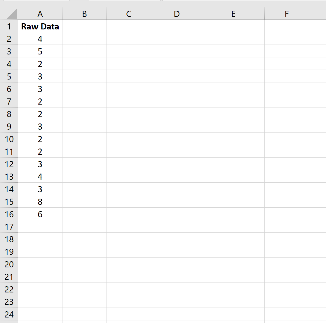
Шаг 1: введите данные
Во-первых, давайте введем значения для набора данных:
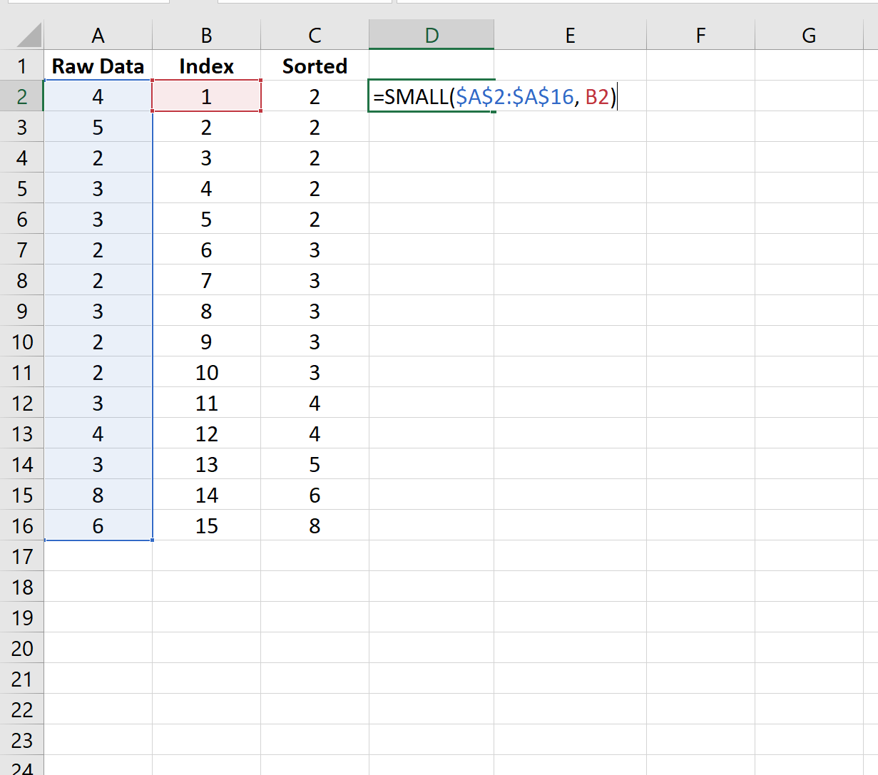
Шаг 2: Сортировка данных
Затем создайте столбец индекса и столбец отсортированных данных:
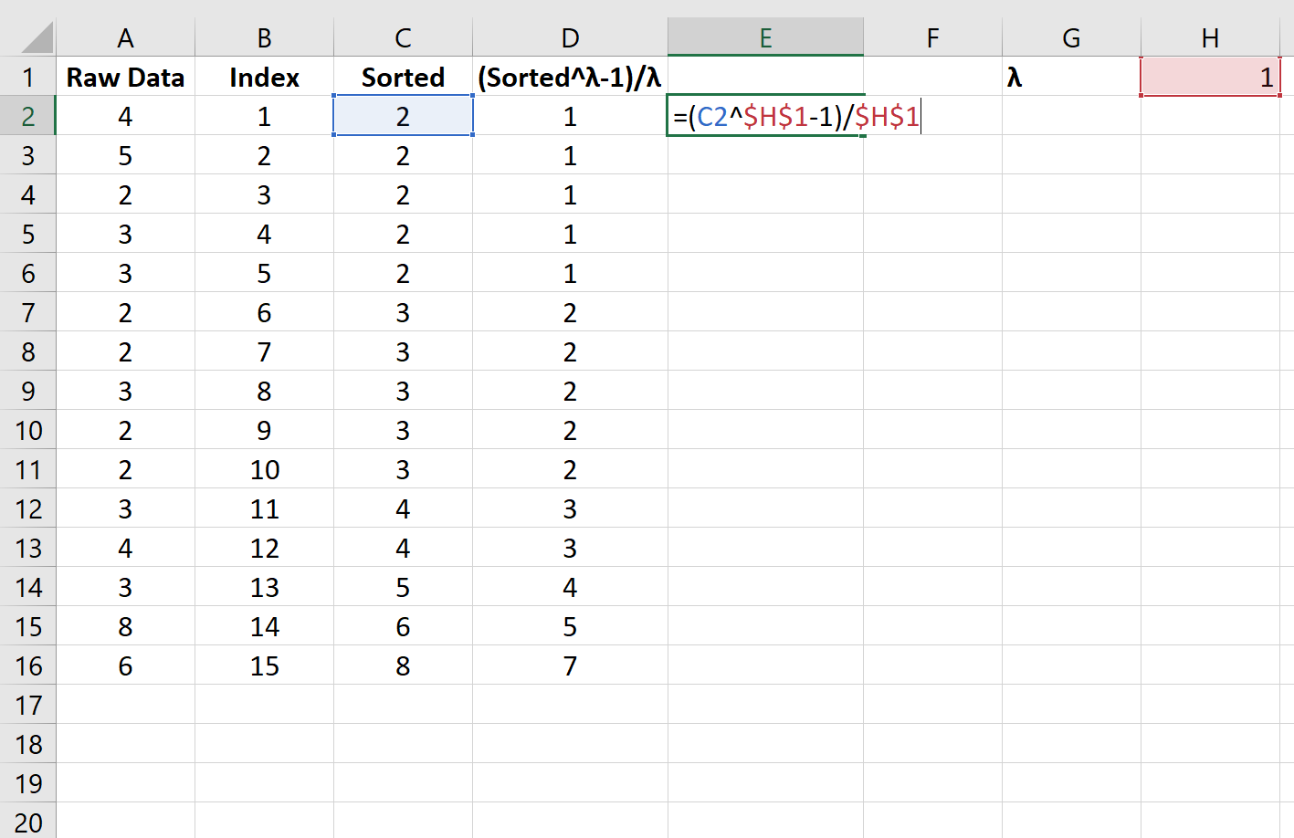
Шаг 3. Выберите произвольное значение для лямбда
Затем мы выберем произвольное значение 1 для лямбда и применим к данным временное преобразование бокса-кокса:
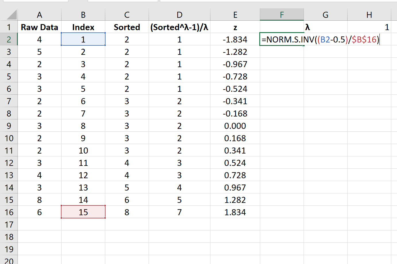
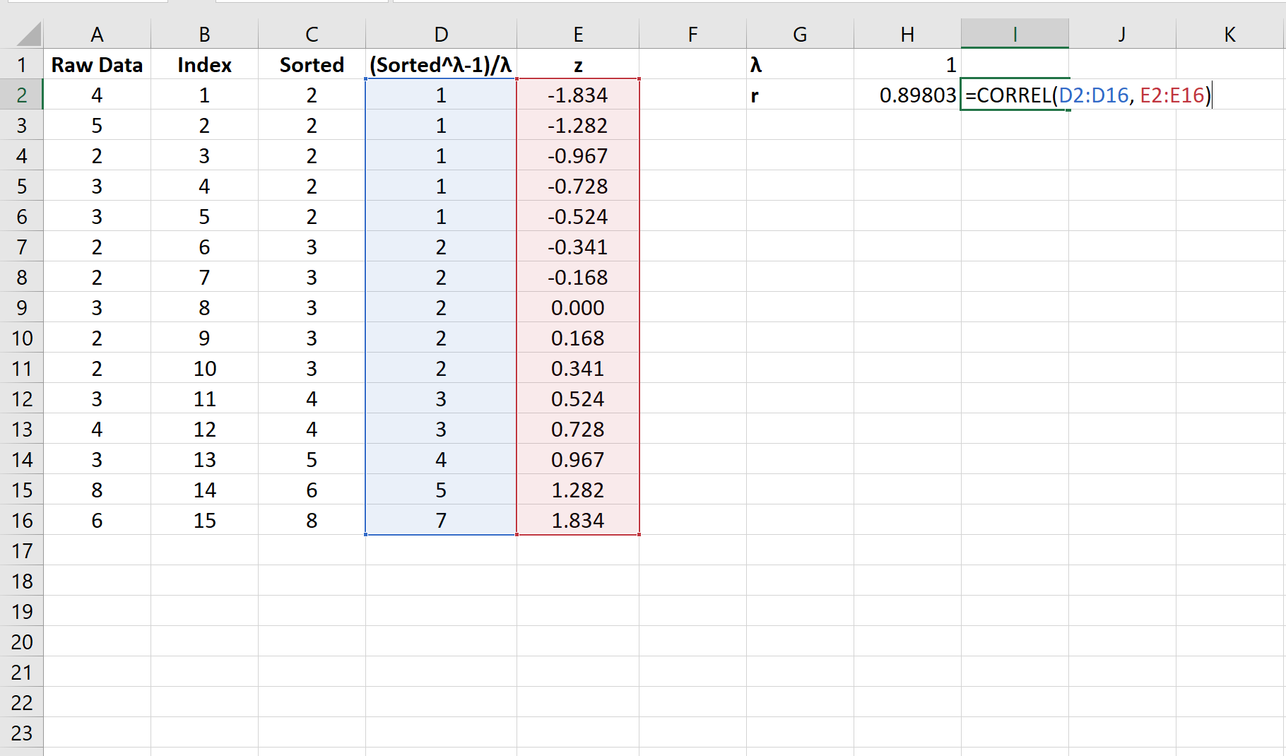
Шаг 4: Рассчитайте Z-показатели
Далее мы рассчитаем z-оценку для каждого значения в индексе:
Затем мы рассчитаем корреляцию между значениями, преобразованными по боксу-коксу, и z-показателями:
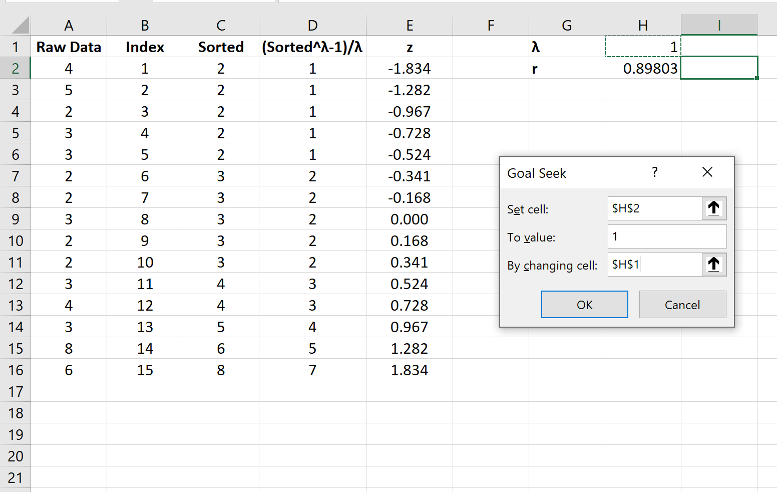
Шаг 5: Найдите оптимальное значение лямбда
Далее мы воспользуемся поиском цели, чтобы найти оптимальное значение лямбда для использования в преобразовании бокса-кокса.
Для этого щелкните вкладку « Данные » на верхней ленте. Затем нажмите «Анализ «что, если»» в группе « Прогноз ».

В раскрывающемся меню нажмите «Поиск цели » и введите следующие значения:
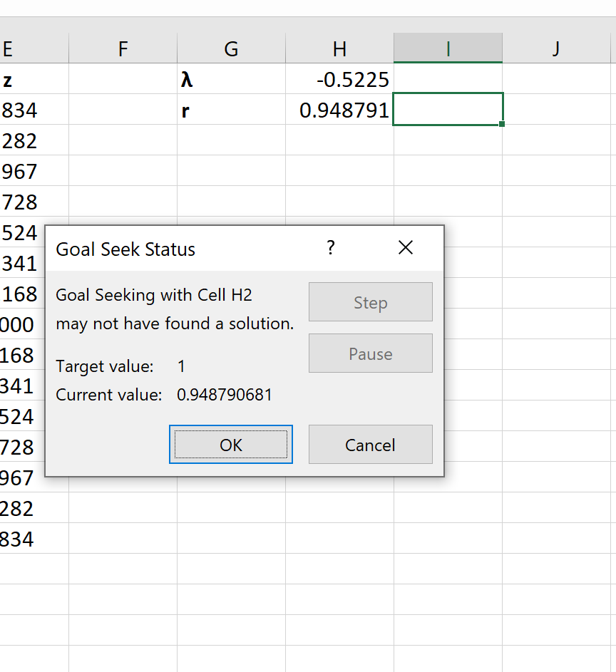
Как только вы нажмете OK , Goal Seek автоматически найдет оптимальное значение лямбда, равное -0,5225 .
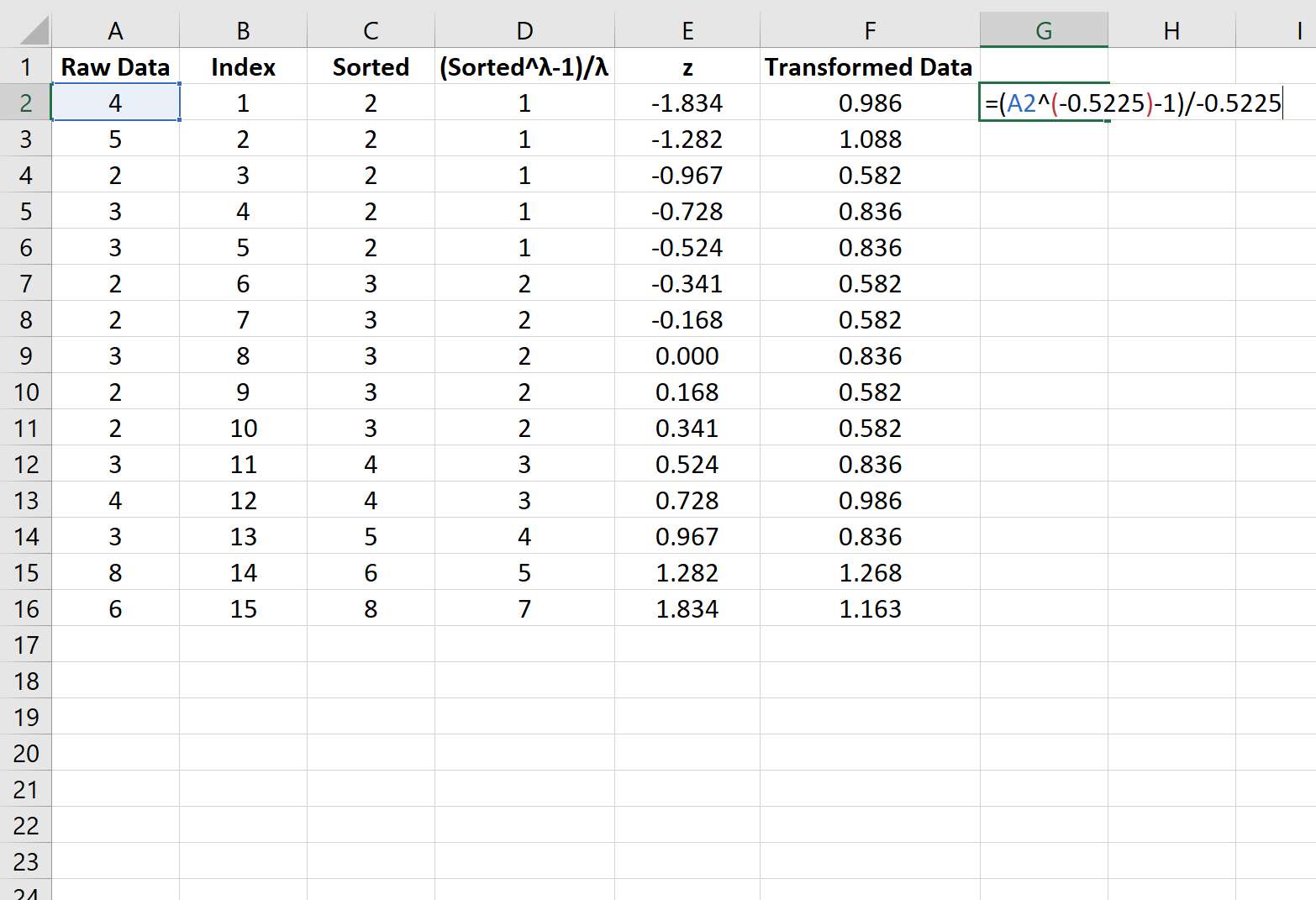
Шаг 6: Выполните преобразование Бокса-Кокса
Наконец, мы применим преобразование бокса-кокса к исходным данным, используя лямбда-значение -0,5225:
Бонус: мы можем подтвердить нормальное распределение преобразованных данных, выполнив тест Харке-Бера в Excel .
Дополнительные ресурсы
Как преобразовать данные в Excel (логарифм, квадратный корень, кубический корень)
Как рассчитать Z-баллы в Excel

Юлия Лайши
Эксперт по предмету «Эконометрика»
преподавательский стаж — 5 лет
Задать вопрос автору статьи
Эконометрика в экономике
Определение 1
Эконометрика – это научное направление, исследующее качественные и количественные связи при использовании статистических моделей и методов.
Основой эконометрического знания стала статистика и математика, которые активно использовались и продолжают применяться в области развития экономической теории. Теоретическое направление эконометрики исследует статистические параметры испытаний и оценок. В свою очередь, ее прикладное направление позволяет изучать и оценивать теории и гипотезы, выдвигаемые в рамках экономической науки.
С помощью эконометрики формируются инструменты для осуществления измерений в экономике, реализуется методология исследования хозяйственных моделей микро- и макроуровней. Эконометрика эффективно применяется для разработки прогнозов. Она является дисциплиной, активно использующей методы статистики и математики, что роднит ее с биометрией, наукометрией, психометрией и другими прикладными науками.
![]()
Сделаем домашку
с вашим ребенком за 380 ₽
Уделите время себе, а мы сделаем всю домашку с вашим ребенком в режиме online
Бесплатное пробное занятие
*количество мест ограничено
Одним из новейших направлений эконометрики является непараметрическая эконометрика. Она не требует спецификации форм, так как данные исследуемых объектом сами формируют модели. Такой подход представляет собой оптимальный метод исследования практических задач. Он позволяет оценить большой объем данных при относительно малом количестве заданных переменных. Методы непараметрической эконометрики применяются там, где не работают классические методики.
Сущность метода Бокса-Кокса
Методы эконометрики позволяют оценивать влияние большого числа факторов на статические и динамические модели. Часто возникают ситуации, когда задействованные в исследовании данные не могут пройти тест на нормальность. Под нормальностью статистической выборки понимается частный случай критерия согласия. Для расчетов в математике применяются нормально распределенные величины, под влиянием закона больших чисел. Тест на нормальность проводится на первом этапе исследования. Таким образом, специалист определяет метод проведения основного исследования – параметрический или непараметрический.
«Тест Бокса-Кокса в excel» 👇
Метод Бокса-Кокса позволяет преобразовать исходную «ненормальную» статистику, в «нормальную». Кроме того, он помогает определиться с выбором модели для исследования. Например, линейную или логарифмическую зависимость. Проблема заключается в том, что иногда значения этих подходов могут быть равными, что усложняет выбор исследователя. В случае, если выбор будет сделан неверно, полученный результат может дать существенное отклонение от реальных значений. Тест Бокса-Кокса позволяет выбрать оптимальную модель.
Для описания используют следующую зависимость:

Рисунок 1. Зависимость. Автор24 — интернет-биржа студенческих работ
в случае, если значение переменной равно нулю, то вид является неопределенным.
Предел искомого значения вычисляется следующим образом:

Рисунок 2. Предел. Автор24 — интернет-биржа студенческих работ
Расчет лимита позволяет заменить регрессионную зависимость более общей. Появляется возможность оценить параметры уравнения методом максимального правдоподобия. А уже после этого для параметров можно определять различные гипотезы.
Тест Бокса-Кокса в Excel
Тест Бокса-Кокса реализован в Stata. Для того, чтобы произвести вычисления, необходимо выполнить следующую последовательность шагов:
- Выгрузить данные в программу Excel.
- Далее используется тест Box-Cox, который вшит в программное обеспечение. Его можно найти, выполняя следующие шаги Menu Statistics – Linear model and related.
- Реализация в Excel теста Бера-МакАлера и РЕ-теста МакКиннона.
- Проверка логарифмической функции с помощью гипотезы постоянства, используя t-статистику.
- Проверка фиктивного значения переменной, влияющей на сдвиг и наклон графического изображения функции.
- Подтвердить незначительность коэффициента.
- Расчет искомой величины должен осуществляться с учетом отклонения.
Исходя из этапов построения модели, можно определить следующие параметры вычислений: определить изменение регрессии под влиянием фиктивной переменной, либо сопоставление результатов выборов различных фиктивных переменных. Эта переменная может использоваться для построения и анализа временного ряда.
Находи статьи и создавай свой список литературы по ГОСТу
Поиск по теме
A box-cox transformation is a commonly used method for transforming a non-normally distributed dataset into a more normally distributed one.
The basic idea is to find some value for λ such that the transformed data is as close to normally distributed as possible, using the following formula:
- y(λ) = (yλ – 1) / λ if y ≠ 0
- y(λ) = log(y) if y = 0
The following step-by-step example shows how to perform a box-cox transformation on a dataset in Excel.
Step 1: Enter the Data
First, let’s enter the values for a dataset:

Step 2: Sort the Data
Next, create an index column and a column of sorted data:

Step 3: Choose an Arbitrary Value for Lambda
Next, we’ll choose an arbitrary value of 1 for lambda and apply a temporary box-cox transformation to the data:

Step 4: Calculate the Z-Scores
Next, we’ll calculate the z-score for each value in the index:

We’ll then calculate the correlation between the box-cox transformed values and the z-scores:

Step 5: Find the Optimal Lambda Value
Next, we’ll use Goal Seek to find the optimal lambda value to use in the box-cox transformation.
To do so, click the Data tab along the top ribbon. Then click What-If-Analysis within the Forecast group.

In the dropdown menu, click Goal Seek and fill in the following values:

Once you click OK, Goal Seek will automatically find the optimal lambda value to be -0.5225.

Step 6: Perform the Box-Cox Transformation
Lastly, we’ll apply the box-cox transformation to the original data, using a lambda value of -0.5225:

Bonus: We can confirm that the transformed data is normally distributed by performing a Jarque-Bera test in Excel.
Additional Resources
How to Transform Data in Excel (Log, Square Root, Cube Root)
How to Calculate Z-Scores in Excel
We seek a transformation of data in a sample x1, …, xn which results in data that is normally distributed.
If one of the sample values is not positive, then we add 1–a to all the sample values where a is the smallest sample value. This will transform the sample into only positive values. Next, we sort the sample into ascending order, and so assume that x1 ≤ … ≤ xn. We now define the Box-Cox transformation y1, …, yn for any value of λ ≠ 0
![]()
We could also define the transformation at λ = 0, but because
![]()
this is not necessary. In fact, if in the optimization process described below, we get a value of λ close to zero, we will generally use the value λ = 0 to get a ln transformation.
We now use the approach described in Graphical Tests for Normality to create QQ plots by defining a sequence z1, …, zn where
![]()
and Φ-1 is the inverse of the standard normal distribution, i.e. Φ-1(p) = NORM.S.INV(p).
Finally, we use Excel’s Goal Seek to find the value of λ which maximizes the correlation coefficient between the y and z values.
Example 1: Find the Box-Cox transformation which best normalizes the data in range B4:B13 of Figure 1.
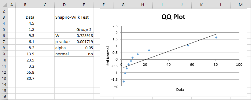
Figure 1 – Non-normal data
As we can see from the QQ plot and the results of the Shapiro-Wilk test, this data is not normal. We now create the x, y and z values for the data, as described above. This is shown in Figure 2.
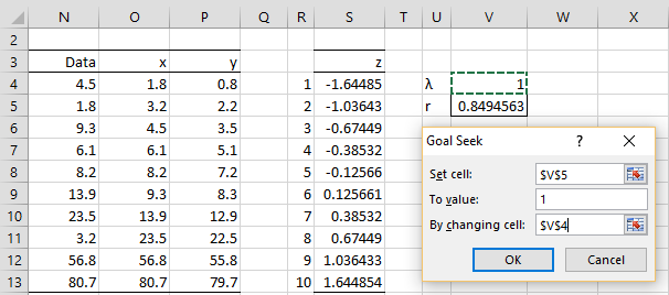
Figure 2 – Set up for Goal Seek
Here, column O consists of the data in sorted order, e.g. by using the formula =QSORT(N4:N13), and column P contains the transformed data, e.g. cell P4 contains the formula =(O4^V$4-1)/V$4 or optionally =IF(V4=0,LN(O4),(O4^V$4-1)/V$4). Column S consists of the inverse normal values, and so cell S4 contains the formula =NORM.S.INV((R4-0.5)/R$13). Finally, cell V4 contains a guess for the λ value and cell V5 contains the formula =CORREL(P4:P13,S4:S13) to calculate the correlation coefficient between the y and z values.
We now select Data > Data Tools|What-If Analysis and choose the Goal Seek tool. Next, we fill in the dialog box that appears with the values shown on the right side of Figure 2 and press the OK button. The result is that the value for λ converges to -0.286629.
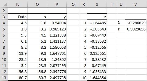
Figure 3 – Goal Seek output
Figure 3 contains the results of the Shapiro-Wilk test and QQ plot on the transformed data in column P of Figure 2. As you can see, the transformed data is normally distributed.

Figure 4 – Testing normality for transformed data
Actually the value λ = -0.216 yields a slightly better correlation, namely r = .9937987, but the normality testing is not much different for this transformation.
Another approach to optimizing the value of lambda is to maximize the log-likelihood function, which in this case is
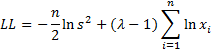
where s2 = the population variance of the transformed xi values, as calculated using the VAR.P(R1) function in Excel. The value of LL can be maximized using Goal Seek or using the golden search algorithm. The Real Statistics Resource Pack has implemented this approach as described in Example 2.
Real Statistics Functions: The Real Statistics Resource Pack provides the following functions:
BOXCOX(R1, λ): array function which returns a range containing the Box-Cox transformation of the data in range R1 using the given lambda value. If the lambda argument is omitted, then the transformation which best normalizes the data in R1 is used, based on maximizing the log-likelihood function.
BOXCOXLL(R1, λ) = log likelihood function of the Box-Cox transformation of the data in R1 using the given lambda value
BOXCOXLambda(R1) = the value of lambda which maximizes the log likelihood function of the Box-Cox transformation of the data in R1
Example 2: Repeat Example 1 using the Real Statistics functions
We begin by displaying the Box-Cox transformation for values of lambda between -2 and 2, as shown in Figure 5. E.g. the transform of the data element when λ = -2 are shown in the range D4:D13, as calculated by the array formula =BOXCOX($B$4:$B$13,D3).
The LL value when λ = -2 is -398802 (cell D14), as calculated by the formula =BOXCOXLL($B$4:$B$13,D3). Alternatively, we could use the formula
=- COUNT(B4:B13)/2*LN(VARP(D4:D13))+(D3-1)*SUMPRODUCT(LN(B4:B13))
We see from Figure 5 that the maximum value of LL occurs somewhere between λ = -.5 and λ = 0. We can make successive guesses to eventually find a value sufficiently close to the value of λ that maximizes LL sufficiently well for our needs. Essentially this is what the BOXCOXLambda function does.

Figure 5 – Box-Cox optimization
In fact, we see that =BOXCOXLambda(B4:B13) = -0.16394 (cell N3) provides this value of lambda, corresponding to LL = -24.8913 (cell N14). The transformation values are shown in range N4:N13, as calculated by the array function =BOXCOX(B4:B13), which is equivalent to the array function =BOXCOX(B4:B13, N3).
Finally, we note that the optimal value λ = -0.286629 that we found in Example 1 yields an LL value which is almost as good (LL = -24.9853), but the LL value for λ = -0.16394 is slightly better.
Dataset for variable transformation
In this tutorial we show how to create transform a variable to be closer to the Normal distribution.
The dataset contains the measurements of waste in the production for 47 batches. We would like to make a regression with several process variables but the hypothesis of Normality of the variable Level of waste is not acceptable. We need to make a transformation of this variable before attempting a multilinear regression. After showing you different options to transform data we will use the Box-Cox transformation of XLSTAT.
The results of the Normality test are displayed bellow.

Variable transformation in XLSTAT
There are several ways to transform data in XLSTAT.
Variable transformation with Microsoft Excel tools
First you can take advantage of Microsoft Excel and use the available function in the software. First place the cursor where you would like to have the results displayed. You will access the menu Insert Function by clicking on the fx icon above the spreadsheet.

Then you can select one of the functions listed under either Financial, Math & Trig, Statistical, Database or XLSTAT (last entry).

This gives you access to a wide range of general transformation.
Variable transformation with XLSTAT tools
In XLSTAT we offer you the opportunity to use some more specific functions. You will find them in the option Preparing data / Variables transformation.

Setting up a Box-Cox transformation
In the dialog box that opens you should first select the variables you wish to transform, in this example we select the variable Level of waste in the column B. Also as the column has a label we tick the option Column labels.
Also we can select the Observation labels option by ticking the box and selecting the column A which contains the identifications of the batches.
The results will be displayed in a new sheet as the option Sheet is selected. If you wish to have them at a specific place select the option Range.
The most general transformation is an unbiased standardization (Standardize (n-1)) as usually people work on a sample and not the full population. However there are more transformations available when you tick the option Other.

Then go on the next tab Transformations that contains the following options:
- Standardize (n): to standardize the variables using the biased standard deviation.
- Center: to center the variables, the average of the resulting variables will be 0.
- 1 / Standard deviation (n-1): to divide the variables by their unbiased standard deviation.
- 1 / Standard deviation (n): to divide the variables by their biased standard deviation.
- Rescale from 0 to 1: to rescale the data from 0 to 1.
- Rescale from 0 to 100: to rescale the data from 0 to 100.
- Binarize (0/1): to convert all values that are not 0 to 1, and leave the 0s unchanged.
- Sign (-1/0/1): to convert all values that are negative to -1, all positive values to 1, and leave the 0s unchanged.
- Arcsin: to transform the data to their arc-sine.
- Box-Cox transformation: to improve the normality of the sample. XLSTAT accepts a fixed value of l, or it can find the value that maximizes the likelihood of the sample, assuming the transformed sample follows a normal distribution.
- Winsorize: to remove data that are not within an interval defined by two percentiles: let p1 and p2 be two values comprised between 0 and 1, such that p1 < p2
Select the option Box-Cox transformation as we are trying to get the variable “Level of waste” closer to a Normal distribution. Also select the option Optimize to let XLSTAT find the best Lambda.

The last tab Missing data help you decide what to do in case of missing data. The option selected by default Do not accept missing data will give you a warning in case of missing data. Leave that option selected.

Click on OK to start the computations.
Results of the Box-Cox transformation
In the result sheet called Variables transformation you will find the Transformed data with the value of Lambda used.

You can now compute the Normality test on those transformed data. As you can see bellow now the transformed variable Level of waste is following a Normal distribution.

Was this article useful?
- Yes
- No