
Событие Worksheet.SelectionChange, используемое в VBA Excel для запуска процедур при выборе диапазона на рабочем листе, в том числе отдельной ячейки.
Синтаксис процедуры, выполнение которой инициируется событием Worksheet.SelectionChange:
|
Private Sub Worksheet_SelectionChange(ByVal Target As Range) ‘Операторы процедуры End Sub |
Эта процедура VBA Excel запускается при смене на рабочем листе выделенного диапазона (SelectionChange). Она должна быть размещена в модуле рабочего листа Excel, смена выбранного диапазона ячеек которого будет инициировать ее запуск.
Аргумент Target — это новый выбранный диапазон на рабочем листе.
Шаблон процедуры можно скопировать и вставить в модуль рабочего листа, но не обязательно. Если открыть модуль нужного листа, выбрать в левом верхнем поле объект Worksheet, шаблон процедуры будет добавлен автоматически:

У объекта Worksheet есть и другие события, которые можно выбрать в правом верхнем поле модуля рабочего листа. Процедура с событием SelectionChange добавляется по умолчанию.
Примеры кода с Worksheet.SelectionChange
Пример разработчика
Замечательный пример дан на сайте разработчика:
|
Private Sub Worksheet_SelectionChange(ByVal Target As Range) With ActiveWindow .ScrollRow = Target.Row .ScrollColumn = Target.Column End With End Sub |
При выборе на листе любого диапазона, в том числе отдельной ячейки, лист автоматически прокручивается по горизонтали и вертикали, пока выделенный диапазон не окажется в верхнем левом углу экрана.
Эта процедура работает и при выборе ячейки через адресную строку (слева над обозначениями столбцов), и при выборе из кода VBA Excel, например:
Выбор одной отдельной ячейки
Инициируем выполнение основных операторов процедуры с событием Worksheet.SelectionChange выбором одной отдельной ячейки:
|
Private Sub Worksheet_SelectionChange(ByVal Target As Range) If Target.Address = «$E$5» Then MsgBox «Выбрана ячейка E5» End If End Sub |
Основной оператор MsgBox "Выбрана ячейка E5" будет выполнен при выборе ячейки E5.
Примечание:
В условии примера используется свойство Address переменной Target, так как в прямом выражении Target = Range("E5") по умолчанию сравниваются значения диапазонов. В результате этого, при выборе другой ячейки со значением, совпадающим со значением ячейки E5, равенство будет истинным и основные операторы будут выполнены, а при выборе более одной ячейки, будет сгенерирована ошибка.
Выбор диапазона с заданной ячейкой
Выполнение основных операторов процедуры при вхождении заданной ячейки в выбранный диапазон:
|
Private Sub Worksheet_SelectionChange(ByVal Target As Range) If Not Intersect(Target, Range(«B3»)) Is Nothing Then MsgBox «Ячейка B3 входит в выбранный диапазон» End If End Sub |
Основной оператор MsgBox "Ячейка B3 входит в выбранный диапазон" будет выполнен при выделении диапазона, в который входит ячейка B3, в том числе и при выделении одной этой ячейки.
Выбор ячейки в заданной строке
Инициируем выполнение основных операторов процедуры с событием Worksheet.SelectionChange выбором любой отдельной ячейки во второй строке:
|
Private Sub Worksheet_SelectionChange(ByVal Target As Range) If Target.Count > 1 Then Exit Sub If Target.Row = 2 Then MsgBox «Выбрана ячейка во второй строке» End If End Sub |
Дополнительный оператор If Target.Count > 1 Then Exit Sub необходим для выхода из процедуры при выделении более одной ячейки. Причина: при выделении произвольного диапазона, ограниченного сверху второй строкой, выражение Target.Row = 2 будет возвращать значение True, и операторы в блоке If ... End If будут выполнены.
Ввод даты в ячейку первого столбца
Автоматическое добавление текущей даты в выбранную ячейку первого столбца при условии, что предыдущая ячейка сверху не пустая, а ячейка снизу – пустая:
|
Private Sub Worksheet_SelectionChange(ByVal Target As Range) If Target.Count > 1 Or Target.Row = 1 Or Target.Row = ActiveSheet.Rows.Count Then Exit Sub If Target.Column = 1 And Target.Offset(—1, 0) <> «» And Target.Offset(1, 0) = «» Then Target = Format(Now, «DD.MM.YYYY») End If End Sub |
Этот код VBA может быть полезен при ведении реестра, базы данных на листе Excel с записью текущей даты в первой колонке.
Условие If Target.Count > 1 Or Target.Row = 1 Or Target.Row = ActiveSheet.Rows.Count Then Exit Sub завершает процедуру при выборе более одной ячейки, при выборе ячейки A1 и при выборе последней ячейки первого столбца.
Выбор ячейки A1 приводит к ошибке при проверке условия Target.Offset(-1, 0) <> "", так как происходит выход за границы диапазона рабочего листа.
Ошибка выхода за пределы рабочего листа происходит и при проверке условия Target.Offset(1, 0) = "", если выбрать последнюю ячейку первой колонки.
Примечание:
Текущая дата будет введена в следующую пустую ячейку первого столбца при переходе к ней от заполненной в том числе нажатием клавиши «Enter».
Пример без отслеживания Target
Если необходимо, чтобы процедура запускалась при любой смене выделенного диапазона, аргумент Target можно не отслеживать:
|
Private Sub Worksheet_SelectionChange(ByVal Target As Range) If [B1] > 100 Then [A1].Interior.Color = vbGreen Else [A1].Interior.Color = vbBlue End If End Sub |
После ввода значения в ячейку B1, можно нажать Enter или кликнуть по любой другой ячейке рабочего листа, и событие Worksheet.SelectionChange сработает.
|
Прошу помочь разобраться в макросе с Target и Intersect |
||||||||
Ответить |
||||||||
Ответить |
||||||||
Ответить |
||||||||
Ответить |
||||||||
Ответить |
||||||||
Ответить |
||||||||
Ответить |
||||||||
Ответить |
||||||||
Ответить |
||||||||
Ответить |
||||||||
Ответить |
||||||||
Ответить |
||||||||
Ответить |
||||||||
Ответить |
||||||||
Ответить |
||||||||
Ответить |
||||||||
Ответить |
||||||||
Ответить |
||||||||
Ответить |
||||||||
Ответить |


Excel VBA Referencing Ranges — Range, Cells, Item, Rows & Columns Properties; Offset; ActiveCell; Selection; Insert
You can refer to or access a worksheet range using properties and methods of the Range object. A Range Object refers to a cell or a range of cells. It can be a row, a column or a selection of cells comprising of one or more rectangular / contiguous blocks of cells. One of the most important aspects in vba coding is referencing and using Ranges within a Worksheet. This section (divided into 2 parts) covers various properties and methods for referencing, accessing & using ranges, divided under the following chapters.
Excel VBA Referencing Ranges — Range, Cells, Item, Rows & Columns Properties; Offset; ActiveCell; Selection; Insert:
Range Property, Cells / Item / Rows / Columns Properties, Offset & Relative Referencing, Cell Address;
Activate & Select Cells; the ActiveCell & Selection;
Entire Row & Entire Column Properties, Inserting Cells/Rows/Columns using the Insert Method;
Excel VBA Refer to Ranges — Union & Intersect; Resize; Areas, CurrentRegion, UsedRange & End Properties; SpecialCells Method:
Ranges — Union & Intersect;
Resize a Range;
Referencing — Contiguous Block(s) of Cells, Range of Contiguous Data, Cells Meeting a Specified Criteria, Used Range, Cell at the End of a Block / Region, Last Used Row or Column;
Related Links:
Working with Objects in Excel VBA
Excel VBA Application Object, the Default Object in Excel
Excel VBA Workbook Object, working with Workbooks in Excel
Microsoft Excel VBA — Worksheets
Excel VBA Custom Classes and Objects
——————————————————————————————-
Contents:
Range Property, Cells / Item / Rows / Columns Properties, Offset & Relative Referencing, Cell Address
Activate & Select Cells; the ActiveCell & Selection
Entire Row & Entire Column Properties, Inserting Cells/Rows/Columns using the Insert Method
——————————————————————————————-
Range Property, Cells / Item / Rows / Columns Properties, Offset & Relative Referencing, Cell Address
A Range Object refers to a cell or a range of cells. It can be a row, a column or a selection of cells comprising of one or more rectangular / contiguous blocks of cells. A Range object is always with reference to a specific worksheet, and Excel currently does not support Range objects spread over multiple worksheets.
Range object refers to a single cell:
Dim rng As Range
Set rng = Range(«A1»)
Range object refers to a block of contiguous cells:
Dim rng As Range
Set rng = Range(«A1:C3»)
Range object refers to a row:
Dim rng As Range
Set rng = Rows(1)
Range object refers to multiple columns:
Dim rng As Range
Set rng = Columns(«A:C»)
Range object refers to 2 or more blocks of contiguous cells — using the ‘Union method’ & ‘Selection’ (these have been explained in detail later in this section).
Union method:
Dim rng1 As Range, rng2 As Range, rngUnion As Range
‘set a contiguous block of cells as the first range:
Set rng1 = Range(«A1:B2»)
‘set another contiguous block of cells as the second range:
Set rng2 = Range(«D3:E4»)
‘assign a variable (range object) to represent the union of the 2 ranges, using the Union method:
Set rngUnion = Union(rng1, rng2)
‘set interior color for the range which is the union of 2 range objects:
rngUnion.Interior.Color = vbYellow
Selection property:
‘select 2 contiguous block of cells, using the Select method:
Range(«A1:B2,D3:E4»).Select
‘perform action (set interior color of cells to yellow) on the Selection, which is a Range object:
Selection.Interior.Color = vbYellow
Range property of the Worksheet object ie. Worksheet.Range Property. Syntax: WorksheetObject.Range(Cell1, Cell2). You have an option to use only the Cell1 argument and in this case it will have to be a A1-style reference to a range which can include a range operator (colon) or the union operator (comma), or the reference to a range can be a defined name. Examples of using this type of reference are Worksheets(«Sheet1»).Range(«A1») which refers to cell A1; or Worksheets(«Sheet1»).Range(«A1:B3») which refers to the cells A1, A2, A3, B1, B2 & B3. When both the Cell1 & Cell2 arguments are used (cell1 and cell2 are Range objects), these refer to the cells at the top-left corner and the lower-right corner of the range (ie. the start and end cells of the range), and these arguments can be a single cell, an entire row or column or a single named cell. An example of using this type of reference is Worksheets(«Sheet1»).Range(Cells(1, 1), Cells(3, 2)) which refers to the cells A1, A2, A3, B1, B2 & B3. Omitting the object qualifier will default to the active sheet viz. using the code Range(«A1») will return cell A1 of the active sheet, and will be the same as using Application.Range(«A1») or ActiveSheet.Range(«A1»).
Range property of the Range object: Use the Range.Range property [Syntax: RangeObject.Range(Cell1,Cell2)] for relative referencing ie. to access a range relative to a range object. For example, Worksheets(«Sheet1»).Range(«C5:E8»).Range(«A1») will refer to Range(«C5») and Worksheets(«Sheet1»).Range(«C5:E8»).Range(«B2») will refer to Range(«D6»).
Shortcut Range Reference: As compared to using the Range property, you can also use a shorter code to refer to a range by using square brackets to enclose an A1-style reference or a name. While using square brackets, you do not type the Range word or wrap the range in quotation marks to make it a string. Using square brackets is similar to applying the Evaluate method of the Application object. The Range property or the Evaluate method use a string argument which enables you to manipulate the string with vba code, whereas using the square brackets will be inflexible in this respect. Examples: using [A1].Value = 5 is equivalent to using Range(«A1»).Value = 5; using [A1:A3,B2:B4,C3:D5].Interior.Color = vbRed is equivalent to Range(«A1:A3,B2:B4,C3:D5»).Interior.Color = vbRed; and with named ranges, [Score].Interior.Color = vbBlue is equivalent to Range(«Score»).Interior.Color = vbBlue. Using square brackets only enables reference to fixed ranges which is a significant shortcoming. Using the Range property enables you to manipulate the string argument with vba code so that you can use variables to refer to a dynamic range, as illustrated below:
Sub DynamicRangeVariable()
‘using a variable to refer a dynamic range.
Dim i As Integer
‘enters the text «Hello» in each cell from B1 to B5:
For i = 1 To 5
Range(«B» & i) = «Hello»
Next
End Sub
The Cells Property returns a Range object referring to all cells in a worksheet or a range, as it can be used with respect to an Application object, a Worksheet object or a Range object. Application.Cells Property refers to all cells in the active worksheet. You can use the code Application.Cells or omit the object qualifier (this property is a member of ‘globals’) and use the code Cells to refer to all cells of the active worksheet. The Worksheet.Cells Property (Syntax: WorksheetObject.Cells) refers to all cells of a specified worksheet. Use the code Worksheets(«Sheet1»).Cells to refer to all cells of worksheet named «Sheet1». Use the Range.Cells Property ro refer to cells in a specified range — (Syntax: RangeObject.Cells). This property can be used as Range(«A1:B5»).Cells, however using the word cells in this case is immaterial because with or without this word the code will refer to the range A1:B5. To refer to a specific cell, use the Item property of the Range object (as explained in detail below) by specifying the relative row and column positions after the Cells keyword, viz. Worksheets(«Sheet1»).Cells.Item(2, 3) refers to range C2 and Worksheets(«Sheet1»).Range(«C2»).Cells(2, 3) will refer to range E3. Because the Item property is the Range object’s default property you can omit the Item word word and use the code Worksheets(«Sheet1»).Cells(2, 3) which also refers to range C2. You may find it preferable in some cases to use Worksheets(«Sheet1»).Cells(2, 3) over Worksheets(«Sheet1»).Range(«C2») because variables for the row and column can easily be used therein.
Item property of the Range object: Use the Range.Item Property to return a range as offset to the specified range. Syntax: RangeObject.Item(RowIndex, ColumnIndex). The Item word can be omitted because Item is the Range object’s default property. It is necessary to specify the RowIndex argument while ColumnIndex is optional. RowIndex is the index number of the cell, starting with 1 and increasing from left to right and then down. Worksheets(«Sheet1»).Cells.Item(1) or Worksheets(«Sheet1»).Cells(1) refers to range A1 (the top-left cell in the worksheet), Worksheets(«Sheet1»).Cells(2) refers to range B1 (cell next to the right of the top-left cell). While using a single-parameter reference of the Item property (ie. RowIndex), if index exceeds the number of columns in the specified range, the reference will wrap to successive rows within the range columns. Omitting the object qualifier will default to active sheet. Cells(16385) refers to range A2 of the active sheet in Excel 2007 which has 16384 columns, and Cells(16386) refers to range B2, and so on. Also note that RowIndex and ColumnIndex are offsets and relative to the specified Range (ie. relative to the top-left corner of the specified range). Both Range(«B3»).Item(1) and Range(«B3:D6»).Item(1) refer to range B3. The following refer to range D4, the sixth cell in the range: Range(«B3:D6»).Item(6) or Range(«B3:D6»).Cells(6) or Range(«B3:D6»)(6). ColumnIndex refers to the column number of the cell, can be a number starting with 1 or can be a string starting with the letter «A». Worksheets(«Sheet1»).Cells(2, 3) and Worksheets(«Sheet1»).Cells(2, «C») both refer to range C2 wherein the RowIndex is 2 and ColumnIndex is 3 (column C). Range(«C2»).Cells(2, 3) refers to range E3 in the active sheet, and Range(«C2»).Cells(4, 5) refers to range G5 in the active sheet. Using Range(«C2»).Item(2, 3) and Range(«C2»).Item(4, 5) has the same effect and will refer to range E3 & range G5 respectively. Using Range(«C2:D3»).Cells(2, 3) and Range(«C2:D3»).Cells(4, 5) will also refer to range E3 & range G5 respectively. Omitting the Item or Cells word — Range(«C2:D3»)(2, 3) and Range(«C2:D3»)(4, 5) also refers to range E3 & range G5 respectively. It is apparant here that you can refer to and return cells outside the original specified range, using the Item property.
Columns property of the Worksheet object: Use the Worksheet.Columns Property (Syntax: WorksheetObject.Columns) to refer to all columns in a worksheet which are returned as a Range object. Example: Worksheets(«Sheet1»).Columns will return all columns of the worksheet; Worksheets(«Sheet1»).Columns(1) returns the first column (column A) in the worksheet; Worksheets(«Sheet1»).Columns(«A») returns the first column (column A); Worksheets(«Sheet1»).Columns(«A:C») returns the columns A, B & C; and so on. Omitting the object qualifier will default to the active sheet viz. using the code Columns(1) will return the first column of the active sheet, and will be the same as using Application.Columns(1).
Columns property of the Range object: Use the Range.Columns Property (Syntax: RangeObject.Columns) to refer to columns in a specified range. Example1: color cells from all columns of the specified range ie. B2 to D4: Worksheets(«Sheet1»).Range(«B2:D4»).Columns.Interior.Color = vbYellow. Example2: color cells from first column of the range only ie. B2 to B4: Worksheets(«Sheet1»).Range(«B2:D4»).Columns(1).Interior.Color = vbGreen. If the specified range object contains multiple areas, the columns from the first area only will be returned by this property (Areas property has been explained in detail later in this section). Take the example of 2 areas in the specified range, first area being «B2:D4» and the second area being «F3:G6» — the following code will color cells from first column of the first area only ie. cells B2 to B4: Worksheets(«Sheet1»).Range(«B2:D4, F3:G6»).Columns(1).Interior.Color = vbRed. Omitting the object qualifier will default to active sheet — following will apply color to column A of the ActiveSheet: Columns(1).Interior.Color = vbRed.
Use the Worksheet.Rows Property (Syntax: WorksheetObject.Rows) to refer to all rows in a worksheet which are returned as a Range object. Example: Worksheets(«Sheet1»).Rows will return all rows of the worksheet; Worksheets(«Sheet1»).Rows(1) returns the first row (row one) in the worksheet; Worksheets(«Sheet1»).Rows(3) returns the third row (row three) in the worksheet; Worksheets(«Sheet1»).Rows(«1:3») returns the first 3 rows; and so on. Omitting the object qualifier will default to the active sheet viz. using the code Rows(1) will return the first row of the active sheet, and will be the same as using Application.Rows(1).
Use the Range.Rows Property (Syntax: RangeObject.Rows) to refer to rows in a specified range. Example1: color cells from all rows of the specified range ie. B2 to D4: Worksheets(«Sheet1»).Range(«B2:D4»).Rows.Interior.Color = vbYellow. Example2: color cells from first row of the range only ie. B2 to D2: Worksheets(«Sheet1»).Range(«B2:D4»).Rows(1).Interior.Color = vbGreen. If the specified range object contains multiple areas, the rows from the first area only will be returned by this property (Areas property has been explained in detail later in this section). Take the example of 2 areas in the specified range, first area being «B2:D4» and the second area being «F3:G6» — the following code will color cells from first row of the first area only ie. cells B2 to D2: Worksheets(«Sheet1»).Range(«B2:D4, F3:G6»).Rows(1).Interior.Color = vbRed. Omitting the object qualifier will default to active sheet — following will apply color to row one of the ActiveSheet: Rows(1).Interior.Color = vbRed.
To refer to a range as offset from a specified range, use the Range.Offset Property. Syntax: RangeObject.Offset(RowOffset, ColumnOffset). Both arguments are optional to specify. The RowOffset argument specifies the number of rows by which the specified range is offset — negative values indicating upward offset and positive values indicating downward offset, with default value being 0. The ColumnOffset argument specifies the number of columns by which the specified range is offset — negative values indicating left offset and positive values indicating right offset, with default value being 0. Examples: Range(«C5»).Offset(1, 2) offsets 1 row & 2 columns and refers to Range E6, Range(«C5:D7»).Offset(1, -2) offsets 1 row downward & 2 columns to the left and refers to Range (A6:B8).
Accessing a worksheet range, with vba code:-
Referencing a single cell:
Enter the value 10 in the cell A1 of the worksheet named «Sheet1» (omitting to mention a property with the Range object will assume the Value property, as shown below):
Worksheets(«Sheet1»).Range(«A1»).Value = 10
Worksheets(«Sheet1»).Range(«A1») = 10
Enter the value of 10 in range C2 of the active worksheet — using Cells(row, column) where row is the row index and column is the column index:
ActiveSheet.Cells(2, 3).Value = 10
Referencing a range of cells:
Enter the value 10 in the cells A1, A2, A3, B1, B2 & B3 (wherein the cells refer to the upper-left corner & lower-right corner of the range) of the active sheet:
ActiveSheet.Range(«A1:B3»).Value = 10
ActiveSheet.Range(«A1», «B3»).Value = 10
ActiveSheet.Range(Cells(1, 1), Cells(3, 2)) = 10
Enter the value 10 in the cells A1 & B3 of worksheet named «Sheet1»:
Worksheets(«Sheet1»).Range(«A1,B3»).Value = 10
Set the background color (red) for cells B2, B3, C2, C3, D2, D3 & H7 of worksheet named «Sheet3»:
ActiveWorkbook.Worksheets(«Sheet3»).
Range(«B2:D3,H7»).Interior.Color = vbRed
Enter the value 10 in the Named Range «Score» of the active worksheet, viz. you can name the Range(«B2:B3») as «Score» to insert 10 in the cells B2 & B3:
Range(«Score»).Value = 10
ActiveSheet.Range(«Score»).Value = 10
Select all the cells of the active worksheet:
ActiveSheet.Cells.Select
Cells.Select
Set the font to «Times New Roman» & the font size to 11, for all the cells of the active worksheet in the active workbook:
ActiveWorkbook.ActiveSheet.Cells.Font.Name = «Times New Roman»
ActiveSheet.Cells.Font.Size = 11
Cells.Font.Size = 11
Referencing Row(s) or Column(s):
Select all the Rows of active worksheet:
ActiveSheet.Rows.Select
Enter the value 10 in the Row number 2 (ie. every cell in second row), of worksheet named «Sheet1»:
Worksheets(«Sheet1»).Rows(2).Value = 10
Select all the Columns of the active worksheet:
ActiveSheet.Columns.Select
Columns.Select
Enter the value 10 in the Column number 3 (ie. every cell in column C), of the active worksheet:
ActiveSheet.Columns(3).Value = 10
Columns(«C»).Value = 10
Enter the value 10 in Column numbers 1, 2 & 3 (ie. every cell in columns A to C), of worksheet named «Sheet1»:
Worksheets(«Sheet1»).Columns(«A:C»).Value = 10
Relative Referencing:
Inserts the value 10 in Range C5 — reference starts from upper-left corner of the defined Range:
Range(«C5:E8»).Range(«A1») = 10
Inserts the value 10 in Range D6 — reference starts from upper-left corner of the defined Range:
Range(«C5:E8»).Range(«B2») = 10
Inserts the value 10 in Range E6 — offsets 1 row & 2 columns, using the Offset property:
Range(«C5»).Offset(1, 2) = 10
Inserts the value 10 in Range(«F7:H10») — offsets 2 rows & 3 columns, using the Offset property:
Range(«C5:E8»).Offset(2, 3) = 10
Example 1 — Using Range, Cells, Columns & Rows property — refer Image 1:

Sub CellsColumnsRowsProperty()
‘using Range, Cells, Columns & Rows property — refer Image 1:
Dim ws As Worksheet
Dim rng As Range
Dim r As Integer, c As Integer, n As Integer, i As Integer, j As Integer
‘set worksheet:
Set ws = Worksheets(«Sheet1»)
‘activate worksheet:
ws.activate
‘enter numbers starting from 1 in each row, for a 5 row & 5 column range (A1:E5):
For r = 1 To 5
n = 1
For c = 1 To 5
Cells(r, c).Value = n
n = n + 1
Next c
Next r
‘set range to A1:E5, wherein the numbers have been entered as above:
Set rng = Range(Cells(1, 1), Cells(5, 5))
‘set background color of each even number column to yellow and of each odd number column to green:
For i = 1 To 5
If i Mod 2 = 0 Then
rng.Columns(i).Interior.Color = vbYellow
Else
rng.Columns(i).Interior.Color = vbGreen
End If
Next i
‘set font color to red and set font to bold for of even number rows:
For j = 1 To 5
If j Mod 2 = 0 Then
rng.Rows(j).Font.Bold = True
rng.Rows(j).Font.Color = vbRed
End If
Next j
‘set font for all cells of the range to italics:
rng.Cells.Font.Italic = True
End Sub
To return the number of the first row in a range, use the Range.Row Property. If the specified range contains multiple areas, this property will return the number of the first row in the first area (Areas property has been explained in detail later in this section). Syntax: RangeObject.Row. To return the number of the first column in a range, use the Range.Column Property. If the specified range contains multiple areas, this property will return the number of the first column in the first area. Syntax: RangeObject.Column.
Examples:
Get the number of the first row in the specified range — returns 4:
MsgBox ActiveSheet.Range(«B4»).Row
MsgBox Worksheets(«Sheet1»).Range(«B4:D7»).Row
Get the number of the first column in the specified range — returns 2:
MsgBox ActiveSheet.Range(«B4:D7»).Column
Get the number of the last row in the specified range — returns 7:
Explanation: Range(«B4:D7»).Rows.Count returns 4 (the number of rows in the range). Range(«B4:D7»).Rows(Range(«B4:D7»).Rows.Count) or Range(«B4:D7»).Rows(4), returns the last row in the specified range.
MsgBox Range(«B4:D7»).Rows(Range(«B4:D7»).
Rows.Count).Row
Example 2: Using Row Property, Column Property & Rows Property, determine row number & column number, and alternate rows — refer Image 2.

Sub RowColumnProperty()
‘Using Row Property, Column Property & Rows Property, determine row number & column number, and alternate rows — refer Image 2.
Dim rng As Range, cell As Range
Dim i As Integer
Set rng = Worksheets(«Sheet1»).Range(«B4:D7»)
‘enter its row number & column number within each cell in the specified range:
For Each cell In rng
cell.Value = cell.Row & «,» & cell.Column
Next
‘set background color of each alternate row of the specified range:
For i = 1 To rng.Rows.count
If i Mod 2 = 1 Then
rng.Rows(i).Interior.Color = vbGreen
Else
rng.Rows(i).Interior.Color = vbYellow
End If
Next
End Sub
Also refer to Example 23, of using the End & Row properties to determine the last used row or column with data.
You can get a Range reference in vba language by using the Range.Address Property, which returns the address of a Range as a string value. This property is read-only.
Examples of using the Address Property:
Returns $B$2:
MsgBox Range(«B2»).Address
Returns $B$2,$C$3:
MsgBox Range(«B2,C3»).Address
Returns $A$1:$B$2,$C$3,$D$4:
Dim strRng As String
Range(«A1:B2,C3,D4»).Select
strRng = Selection.Address
MsgBox strRng
Returns $B2:
MsgBox Range(«B2»).Address(RowAbsolute:=False)
Returns B$2:
MsgBox Range(«B2»).Address(ColumnAbsolute:=False)
Returns R2C2:
MsgBox Range(«B2»).Address(ReferenceStyle:=xlR1C1)
Includes the worksheet (active sheet — «Sheet1») & workbook («Book1.xlsm») name, and returns [Book1.xlsm]Sheet1!$B$2:
MsgBox Range(«B2»).Address(External:=True)
Returns R[1]C[-1] — Range(«B2») is 1 row and -1 columns relative to Range(«C1»):
MsgBox Range(«B2»).Address(RowAbsolute:=False, ColumnAbsolute:=False, ReferenceStyle:=xlR1C1, RelativeTo:=Range(«C1»))
Returns RC[-2] — Range(«A1») is 0 row and -2 columns relative to Range(«C1»):
MsgBox Cells(1, 1).Address(RowAbsolute:=False, ColumnAbsolute:=False, ReferenceStyle:=xlR1C1, RelativeTo:=Range(«C1»))
Activate & Select Cells; the ActiveCell & Selection
The Select method (of the Range object) is used to select a cell or a range of cells in a worksheet — Syntax: RangeObject.Select. Ensure that the worksheet wherein the Select method is applied to select cells, is the active sheet. The ActiveCell Property (of the Application object) returns a single active cell (Range object) in the active worksheet. Remember that the ActiveCell property will not work if the active sheet is not a worksheet. When a cell(s) is selected in the active window, the Selection property (of the Application object) returns a Range object representing all cells which are currently selected in the active worksheet. A Selection may consist of a single cell or a range of multiple cells, but there will only be one active cell within it, which is returned by using the ActiveCell property. When only a single cell is selected, the ActiveCell property returns this cell. On selecting multiple cells using the Select method, the first referenced cell becomes the active cell, and thereafter you can change the active cell using the Activate method. Both the ActiveCell Property & the Selection property are read-only, and not specifying the Application object qualifier viz. Application.ActiveCell or ActiveCell, Application.Selection or Selection, will have the same effect. To activate a single cell within the current selection, use the Activate Method (of the Range object) — Syntax: RangeObject.Activate, and this activated cell is returned by using the ActiveCell property.
We have discussed above that a Selection may consist of a single cell or a range of multiple cells, whereas there can be only one active cell within the Selection. When you activate a cell outside the current selection, the activated cell becomes the only selected cell. You can also use the Activate method to specify a range of multiple cells, but in effect only a single cell will be activated, and this activated cell will be the top-left corner cell of the range specified in the method. If this top-left cell lies within the selection, the current selection will not change, but if this top-left cell lies outside the selection, then the specified range in the Activate method becomes the new selection.
See below codes which illustrate the concepts of ActiveCell and Selection.
Selection containing a range of cells, and the active cell:
‘selects range C1:F5:
Range(«C1:F5»).Select
‘returns C1, the first referenced cell, as the active cell:
MsgBox ActiveCell.Address
Selection containing a range of cells, and the active cell:
‘selects range C1:F5:
Range(«F5:C1»).Select
‘returns C1, the first referenced cell, as the active cell:
MsgBox ActiveCell.Address
Selection containing a range of cells, and the active cell:
‘selects range C1:F5:
Range(«C5:F1»).Select
‘returns C1, the first referenced cell, as the active cell:
MsgBox ActiveCell.Address
Activate a cell within the current selection:
‘selects range B6:F10:
Range(«B6:F10»).Select
‘returns B6, the first referenced cell, as the active cell:
MsgBox ActiveCell.Address
‘selection remains same — range B6:F10, but the active cell is now C8:
Range(«C8»).Activate
MsgBox ActiveCell.Address
Activate a cell outside the current selection:
‘selects range B6:F10:
Range(«B6:F10»).Select
‘returns B6, the first referenced cell, as the active cell:
MsgBox ActiveCell.Address
‘both the selection and the active cell is now A2:
Range(«A2»).Activate
MsgBox ActiveCell.Address
Select a cell within the current selection:
‘selects range B6:F10:
Range(«B6:F10»).Select
‘returns B6, the first referenced cell, as the active cell:
MsgBox ActiveCell.Address
‘both the selection and the active cell is now C8:
Range(«C8»).Select
MsgBox ActiveCell.Address
Activate a range of cells whose top-left cell is within the current selection:


‘selects range B6:F10 — refer Image 3a:
Range(«B6:F10»).Select
‘returns B6, the first referenced cell, as the active cell:
MsgBox ActiveCell.Address
‘selection remains same — range B6:F10, but the active cell is now C8 — refer Image 3b:
Range(«C8:G12»).Activate
MsgBox ActiveCell.Address
Activate a range of cells whose top-left cell is outside the current selection:

‘selects range B6:F10 — refer Image 3a:
Range(«B6:F10»).Select
‘returns B6, the first referenced cell, as the active cell:
MsgBox ActiveCell.Address
‘selection range changes to range B1:F8, and the active cell is now B1 — refer Image 3c:
Range(«B1:F8»).Activate
MsgBox ActiveCell.Address
Using the Application.Selection Property returns the selected object wherein the selection determines the returned object type. Where the selection is a range of cells, this property returns a Range object, and this Selection — which is a Range object — can comprise of a single cell, or multiple cells or multiple non-contiguous ranges. And as mentioned above, the Select method (of the Range object) is used to select a cell or a range of cells in a worksheet. Therefore, after selecting a range, you can perform actions on the selection of cells by using the Selection object. See below illustration.
Sub SelectionObject()
‘select cells in the active sheet using the Range.Select method:
Range(«A1:B3,D6»).Select
‘perform action (set interior color of cells to red) on the Selection, which is a Range object:
Selection.Interior.Color = vbRed
End Sub
Entire Row & Entire Column Properties, Inserting Cells/Rows/Columns using the Insert Method
Use the Range.EntireRow Property to return an entire row or rows within which the specific range is contained. Using this property returns a Range object referring to the entire row(s). Syntax: RangeObject.EntireRow. Use the Range.EntireColumn Property to return an entire column or columns within which the specific range is contained. Using this property returns a Range object referring to the entire column(s). Syntax: RangeObject.EntireColumn.
Examples of using the EntireRow & EntireColumn Properties
Selects row no. 2:
Range(«A2»).EntireRow.Select
Selects row nos. 2, 3 & 4:
Range(«A2:C4»).EntireRow.Select
Enters value 3 in range A3 ie. in the first cell of row no. 3:
Cells(3, 4).EntireRow.Cells(1, 1).Value = 3
Selects column A:
Range(«A2»).EntireColumn.Select
Selects columns A to C:
Range(«A2:C4»).EntireColumn.Select
Enters value 4 in range D1 ie. in the first cell of column no. 4:
Cells(3, 4).EntireColumn.Cells(1, 1).Value = 4
Use the Range.Insert Method to insert a cell or a range of cells in a worksheet. Syntax: RangeObject.Insert(Shift, CopyOrigin). Both arguments are optional to specify. When you insert cell(s) the other cells are shifted to make way, and you can set a value for the Shift argument to determine the direction in which the other cells are shifted — specifying xlShiftDown (value -4121) will shift the cells down, and xlShiftToRight (value -4161) shifts the cells to the right. Omitting this argument will decide the shift direction based on the shape of the range. Specifying xlFormatFromLeftOrAbove (value 0) for the CopyOrigin argument will copy the format for inserted cell(s) from the above cells or cells to the left, and specifying xlFormatFromRightOrBelow (value 1) will copy format from the below cells or cells to the right.
Illustrating Range.Insert Method — for start data refer Image 4a:


Shifts cells down and copies formatting of inserted cell from above cell — refer image 4b:
Range(«B2»).Insert

Shifts cells to the right and copies formatting of inserted cells from cells to the left — refer image 4c:
Range(«B2:C4»).Insert

Shifts cells down and copies formatting of inserted cells from above cells — refer image 4d:
Range(«B2:D3»).Insert

Shifts cells down and copies formatting of inserted cells from below cells — refer image 4e:
Range(«B2:D3»).Insert CopyOrigin:=xlFormatFromRightOrBelow

Shifts cells to the right and copies formatting of inserted cells from cells to the left — refer image 4f:
Range(«B2:D3»).Insert shift:=xlShiftToRight

Shifts cells to the right and copies formatting of inserted cells from cells to the right — refer image 4g:
Range(«B2:D3»).Insert shift:=xlShiftToRight, CopyOrigin:=xlFormatFromRightOrBelow

Inserts 2 rows — row no 2 & 3 — and copies formatting of inserted rows from above cells — refer image 4h:
Range(«B2:D3»).EntireRow.Insert
Below are some illustrations of inserting entire row(s) or column(s) dynamically in a worksheet.
Example 3: Insert row or column — specify the row / column to insert.
Sub InsertRowColumn()
‘Insert row or column — specify the row / column to insert:
Dim ws As Worksheet
Set ws = Worksheets(«Sheet1»)
‘NOTE: each of the below codes need to be run individually.
‘specify the exact row number to insert — insert a row as row no 12:
ws.Rows(12).Insert
‘specify the range below which to insert a row — insert a row below range C3 ie. as row no 4.
ws.Range(«C3»).EntireRow.Offset(1, 0).Insert
‘specify the exact column number to insert — insert a column as column no 4:
ws.Columns(4).Insert
‘specify the range to the right of which to insert a column — insert a column to the right of range C3 ie. as column no 4.
ws.Range(«C3»).EntireColumn.Offset(0, 1).Insert
End Sub
Example 4: Insert row(s) after a specified value is found.
Sub InsertRow1()
‘insert row(s) after a specified value is found:
Dim ws As Worksheet
Dim rngFind As Range, rngSearch As Range, rngLastCell As Range
Dim lFindRow As Long
Set ws = Worksheets(«Sheet1»)
‘find a value after which to insert a row:
Set rngSearch = ws.Range(«A1:E100»)
‘begin search AFTER the last cell in search range (this will start serach from the first cell in search range):
Set rngLastCell = rngSearch.Cells(rngSearch.Cells.count)
Set rngFind = rngSearch.Find(What:=«ExcelVBA», After:=rngLastCell, LookIn:=xlValues, lookat:=xlWhole)
‘exit procedure if value not found:
If Not rngFind Is Nothing Then
lFindRow = rngFind.Row
MsgBox lFindRow
Else
MsgBox «Value not found!»
Exit Sub
End If
‘NOTE: each of the below codes need to be run individually.
‘if value found is in row no 12, one row will be inserted below as row no 13:
ws.Cells(lFindRow + 1, 1).EntireRow.Insert
‘if value found is in row no 12, one row will be inserted 3 rows below (as row no 15):
ws.Cells(lFindRow + 3, 1).EntireRow.Insert
‘if value found is in row no 12, one row will be inserted 3 rows below (as row no 15):
ws.Cells(lFindRow, 1).Offset(3).EntireRow.Insert
‘if value found is in row no 12, 3 rows will be inserted above (as row nos 12, 13 & 14) and the value found row 12 will be pushed down to row 15:
ws.Cells(lFindRow, 1).EntireRow.Resize(3).Insert
‘alternate:
ws.Range(Cells(lFindRow, 1), Cells(lFindRow + 2, 1)).EntireRow.Insert
‘alternate:
ws.Rows(lFindRow & «:» & lFindRow + 2).EntireRow.Insert Shift:=xlDown
‘if value found is in row no 12, 3 rows will be inserted below (as row nos 13, 14 & 15) and the value found row 12 will remain at the same position:
ws.Cells(lFindRow + 1, 1).EntireRow.Resize(3).Insert
‘alternate:
ws.Range(ws.Cells(lFindRow + 1, 1), ws.Cells(lFindRow + 3, 1)).EntireRow.Insert
‘if value found is in row no 12, 3 rows will be inserted after row no 13 (as row nos 14, 15 & 16) and existing rows 12 & 13 will remain at the same position:
ws.Cells(lFindRow + 2, 1).EntireRow.Resize(3).Insert
End Sub
Example 5: Insert a row, n rows above the last used row.
Sub InsertRow2()
‘insert a row, n rows above the last used row
Dim ws As Worksheet
Dim lRowsC As Long
Set ws = Worksheets(«Sheet1»)
‘determine the last used row in a column (column A):
lRowsC = ws.Cells(Rows.count, «A»).End(xlUp).Row
MsgBox lRowsC
‘set n to the no of rows above the last used row:
n = 5
‘check if there are enough rows before the last used row, else you will get an error:
If lRowsC >= n Then
‘insert a row, n rows above the last used row — if last used row is no 5 before insertion, then insert as row no 1 and the last used row will become no 6 (similarly, if last used row is 27, then insert as row no 23) :
ws.Rows(lRowsC).Offset(-n + 1, 0).EntireRow.Insert
Else
MsgBox «Not enough rows before the last used row!»
End If
End Sub
Example 6: Insert a row each time the searched value is found in a range.
For live code of this example, click to download excel file.
Sub InsertRow3()
‘search value in a range and insert a row each time the value is found.
‘you can set the search range with the variable rngSearch in below code — the code will look within this range to find the value below which row is to be inserted.
Dim ws As Worksheet
Dim rngFind As Range, rngSearch As Range, rngLastCell As Range
Dim strAddress As String
Set ws = Worksheets(«Sheet1»)
‘set search range:
Set rngSearch = ws.Range(«A1:K100»)
MsgBox «Searching for ‘ExcelVBA’ within range: » & rngSearch.Address
‘begin search AFTER the last cell in search range
Set rngLastCell = rngSearch.Cells(rngSearch.Cells.count)
‘find value in specified range, starting search AFTER the last cell in search range:
Set rngFind = rngSearch.Find(What:=«ExcelVBA», After:=rngLastCell, LookIn:=xlValues, lookat:=xlWhole)
If rngFind Is Nothing Then
MsgBox «Value not found!»
Exit Sub
Else
‘save cell address of first value found:
strAddress = rngFind.Address
Do
‘find next occurrence of value:
Set rngFind = rngSearch.FindNext(After:=rngFind)
‘insert row below when value is found (if value is found twice in a row, then 2 rows will be inserted):
rngFind.Offset(1).EntireRow.Insert
‘loop till reaching the first value found range:
Loop While rngFind.Address <> strAddress
End If
End Sub
Example 7: Insert rows (user-defined number) within consecutive values found in a column — refer Images 5a & 5b.
For live code of this example, click to download excel file.


Sub InsertRow4()
‘insert rows (user-defined number) wherever 2 consecutive values are found in a column.
‘set column number in which 2 consecutive values are checked to insert rows, using the variable lCellColumn in below code.
‘set row number from where to start searching consecutive values, using the variable lCellRow in below code.
‘refer Image 5a which shows raw data, and Image 5b after this procedure is executed — a single row (lRowsInsert value entered as 1 in input box) is inserted where consecutive values appear in column 1:
Dim ws As Worksheet
Dim lLastUsedRow As Long, lRowsInsert As Long, lCellRow As Long, lCellColumn As Long
Dim rng As Range
Set ws = Worksheets(«Sheet1»)
ws.Activate
‘set column number in which 2 consecutive values are checked to insert rows:
lCellColumn = 1
‘set row number from where to start searching consecutive values:
lCellRow = 1
‘determine the last used row in the column (column no. lCellColumn):
lLastUsedRow = Cells(Rows.count, lCellColumn).End(xlUp).Row
‘enter number of rows to insert between 2 consecutive values:
lRowsInsert = InputBox(«Enter number of rows to insert»)
If lRowsInsert < 1 Then
MsgBox «Error — please enter a value equal to or greater than 1»
Exit Sub
End If
MsgBox «This code will insert » & lRowsInsert & » rows, wherever consecutive values are found in column number » & lCellColumn & «, starting search from row number » & lCellRow
‘loop till the row number equals the last used row (ie. loop right till the end value in the column):
Do While lCellRow < lLastUsedRow
Set rng = Cells(lCellRow, lCellColumn)
‘in case of 2 consecutive values:
If rng <> «» And rng.Offset(1, 0) <> «» Then
‘enter the user-defined number of rows:
Range(rng.Offset(1, 0), rng.Offset(lRowsInsert, 0)).EntireRow.Insert
lCellRow = lCellRow + lRowsInsert + 1
‘determine the last used row — it is dynamic and changes on insertion of rows:
lLastUsedRow = Cells(Rows.count, lCellColumn).End(xlUp).Row
‘alternate method to determine the last used row, when number of rows inserted is fixed — this is faster than using End(xlUp):
‘lLastUsedRow = lLastUsedRow + lRowsInsert + 1
‘MsgBox lLastUsedRow
Else
lCellRow = lCellRow + 1
End If
Loop
End Sub
Ranges are a key concept in Excel, and knowing how to work with them is essential for anyone who wants to program or automate their work using Excel VBA.
In this tutorial, we’ll take a look at how to work with Excel ranges in VBA. We’ll start by discussing what a Range object is. Then, we’ll look at the different ways of referencing a range. Lastly, we’ll explore various examples of how to work with ranges using VBA code.
Excel VBA: The Range object
The Excel VBA Range object is used to represent a range in a worksheet. A range can be a cell, a group of cells, or even all the 17,179,869,184 cells in a sheet.
When programming with Excel VBA, the Range object is going to be your best friend. That’s because much of your work will focus on manipulating data within sheets. Understanding how to work with the Range object will make it easier for you to perform various actions on cells, such as changing their values, sorting, or doing a copy-paste.
The following is the Excel object hierarchy:
Application > Workbook > Worksheet > Range
You can see that the Excel VBA Range object is a property of the Worksheet object. This means that you can access a range by specifying the name of the sheet and the cell address you want to work with. When you don’t specify a sheet name, by default Excel will look for the range in the active sheet. For example, if Sheet1 is active, then both of these lines will refer to the same cell range:
Range("A1")
Worksheets("Sheet1").Range("A1")
Let’s have a closer look at how to reference a range in the section below.


Referencing a range of cells in Excel VBA
Referring to a Range object in Excel VBA can be done in several ways. We’ll discuss the basic syntax and some alternatives that you might want to use, depending on your needs.
Excel VBA: Syntax for specifying a cell range
To refer to a range that consists of one cell, for example, cell D5, you can use the syntax below:
Range("D5")
To refer to a range of cells, you have two acceptable syntaxes. For example, A1 through D5 can be specified using any one below:
Range("A1:D5")
Range("A1", "D5")
To refer to a range outside the active sheet, you need to include the worksheet name. Here’s an example:
Worksheets("Sheet1").Range("A1:D5")
To refer to an entire row, for example, Row 5:
Range("5:5")
To refer to an entire column, for example, Column D:
Range("D:D")
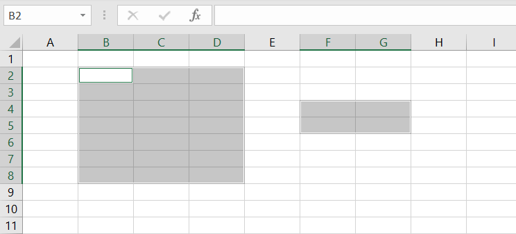
Excel VBA also allows you to refer to multiple ranges at once by using a comma to separate each area. For example, see the below syntax used for referring to all ranges shown in the image:
Range("B2:D8, F4:G5")
Tip: Notice that all of the syntaxes above use double quotes to enclose the range address. To make it quicker for you to type, you can use shortcuts that involve using square brackets without quotes, as shown in the table below:
| Syntax | Shortcut |
|---|---|
Range("D5") |
[D5] |
Range("A1:D5") |
[A1:D5] |
Range("5:5") |
[5:5] |
Range("B2:D8, F4:G5") |
[B2:D8, F4:G5] |
Excel VBA: Referencing a named range
You have probably already used named ranges in your worksheets. They can be found under Name Manager in the Formulas tab.
To refer to a range named MyRange, use the following code:
Range("MyRange")
Remember to enclose the range’s name in double quotes. Otherwise, Excel thinks that you’re referring to a variable.
Alternatively, you can also use the shortcut syntax discussed previously. In this case, double quotes aren’t used:
[MyRange]
Excel VBA: Referencing a range using the Cells property
Another way to refer to a range is by using the Cells property. This property takes two arguments:
Cells(Row, Column)
You must use a numeric value for Row, but you may use either a numeric or string value for Column. Both of these lines refer to cell D5:
Cells(5, "D")
Cells(5, 4)
The advantage of using the Cells property to refer to ranges becomes clear when you need to loop through rows or columns. You can create a more readable piece of code by using variables as the Cells arguments in a looping.
Excel VBA: Referencing a range using the Offset property
The Offset property provides another handy means for referring to ranges. It allows you to refer to a cell based on the location of another cell, such as the active cell.
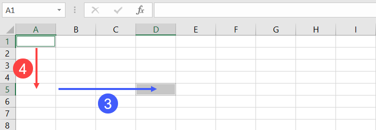
Like the Cells property, the Offset property has two parameters. The first determines how many rows to offset, while the second represents the number of columns to offset. Here is the syntax:
Range.Offset(RowOffset, ColumnOffset)
For example, the following code refers to cell D5 from cell A1:
Range("A1").Offset(4,3)
The negative numbers refer to cells that are above or below the range of values. For example, a -2 row offset refers to two rows above the range, and a -1 column offset refers to a column to the left of the range. The following example refers to cell A1:
Range("D3").Offset(-2, -3)
If you need to go over only a row or a column, but not both, you don’t have to enter both the row and the column parameters. You can also use 0 as one or both of the arguments. For example, the following lines refer to D5:
Range("D5").Offset(0, 0)
Range("D2").Offset(3, 0)
Range("G5").Offset(, -3)
Let’s take a look at some of the most common range examples. These examples will show you how to use VBA to select and manipulate ranges in your worksheets. Some of these examples are complete procedures, while others are code snippets that you can just copy-paste to your own Sub to try.
Excel VBA: Select a range of cells
To select a range of cells, use the Select method.
The following line selects a range from A1 to D5 in the active worksheet:
Range("A1:D5").Select
To select a range from A1 to the active cell, use the following line:
Range("A1", ActiveCell).Select
The following code selects from the active cell to 3 rows below the active cell and five columns to the right:
Range(ActiveCell, ActiveCell.Offset(3, 5)).Select
It’s important to note that when you need to select a range on a specific worksheet, you need to ensure that the correct worksheet is active. Otherwise, an error will occur. For example, you want to select B2 to J5 on Sheet1. The following code will generate an error if Sheet1 is not active:
Worksheets("Sheet1").Range("B2:J5").Select
Instead, use these two lines of code to make your code work as expected:
Worksheets("Sheet1").Activate
Range("B2:J5").Select
Excel VBA: Set values to a range
The following statement sets a value of 100 into cell C7 of the active worksheet:
Range("C7").Value = 100
The Value property allows you to represent the value of any cell in a worksheet. It’s a read/write property, so you can use it for both reading and changing values.
You can also set values of a range of any size. The following statement enters the text “Hello” into each cell in the range A1:C7 in Sheet2:
Worksheets("Sheet2").Range("A1:C7").Value = "Hello"
Value is the default property for a Range object. This means that if you don’t provide any properties in your range, Excel will use this Value property.
Both of the following lines enter a value of 100 into cell C7 of the active worksheet:
Range("C7").Value = 100
Range("C7") = 100
Excel VBA: Copy range to another sheet
To copy and paste a range in Excel VBA, you use the Copy and Paste methods. The Copy method copies a range, and the Paste method pastes it into a worksheet. It might look a bit complicated but let’s see what each does with an example below.
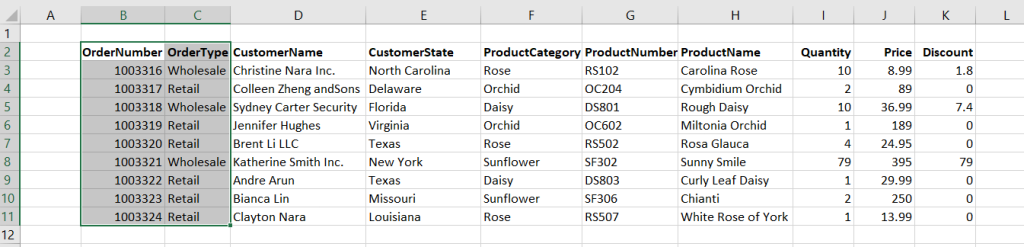
Let’s say you have Orders data, as shown in the below screenshot, which is imported from Airtable every day using Coupler.io. This tool allows users to do it automatically on the schedule they want with just a few clicks and no coding required.

In addition, they can combine data from other different sources (such as Jira, Mailchimp, etc.) into one destination for analysis purposes.

As you can see, the data starts from B2. You want to copy only range B2:C11 and paste them to Sheet2 at the same address. The following is an example Sub you can use:
Sub CopyRangeToAnotherSheet()
    Sheets("Sheet1").Activate
    Range("B2:C11").Select
    Selection.Copy

    Sheets("Sheet2").Activate
    Range("B2").Select
    ActiveSheet.Paste
End Sub
Alternatively, you can also use a single line of code as shown below:
Sub CopyRangeToAnotherSheet2()
    Worksheets("Sheet1").Range("B2:C11").Copy Worksheets("Sheet2").Range("B2")
End Sub
The above Sub procedure takes advantage of the fact that the Copy method can use an argument that corresponds to the destination range for the copy operation. Notice that actually, you don’t have to select a range before doing something with it.
Excel VBA: Dynamic range example
In many cases, you may need to copy a range of cells but don’t know exactly how many rows and columns it has. For example, if you use Coupler.io or other integration tools to import data from an external app into Excel on a daily schedule, the number of rows may change over time.
How can you determine this dynamic range? One solution is to use the CurrentRegion property. This property returns an Excel VBA Range object within its boundaries. As long as the data is surrounded by one empty row and one empty column, you can select it with CurrentRegion.
The following line selects the contiguous range around Cell B2:
Range("B2").CurrentRegion.Select

Now, let’s say you want to select only Columns B and C of the range, and from the second row, you can use the following line:
Range("B2", Range("C2").End(xlDown)).Select
You can now do whatever you want with your selected range — copy or move it to another sheet, format it, and so on.
If you want to find the last row of a used range using Excel VBA, it’s also possible without selecting anything. Here’s the line you can use to find the row number of Column B’s last row data:
' Find the row number of Column B's last row data
RowNumOfLastRow = Cells(Rows.Count, 2).End(xlUp).Row


' Result: 11
MsgBox RowNumOfLastRow
Excel VBA: Loop for each cell in a range
For looping each cell in a range, the For Each loop is an excellent choice. This type of loop is great for looping through a collection of objects such as cells in a range, worksheets in a workbook, or other collections.
The following procedure shows how to loop through each cell in Range B2:K11. We use an object variable named Obj, which refers to the cell being processed. Within the loop, the code checks if the cell contains a formula and then sets its color to blue.
Sub LoopForEachCell()
    Dim obj As Range
    For Each obj In Range("B2:K11")
        If obj.HasFormula Then obj.Font.Color = vbBlue
    Next obj
End Sub
Excel VBA: Loop for each row in a range
When looping through rows (or columns), you can use the Cells property to refer to a range of cells. This makes your code more readable compared to when you’re using the Range syntax.
For example, to loop for each row in range B2:K11 and bold all the cells from Column I to K, you might write a loop like this:
Sub LoopForEachRow()
    For i = 1 To 11
        Range("I" & i & ":K" & i).Font.Bold = True
    Next i
End Sub
Instead of typing in a range address, you can use the Cells property to make the loop easier to read and write. For example, the code below uses the Cells and Resize properties to find the required cell based on the active cell:
Sub LoopForEachRow2()
    For i = 1 To 11
        Cells(i, "I").Resize(, 3).Font.Bold = True
    Next i
End Sub
Excel VBA: Clear a range
There are three ways to clear a range in Excel VBA.
The first is to use the Clear method, which will clear the entire range, including cell contents and formatting.
The second is to use the ClearContents method, which will clear the contents of the range but leave the formatting intact.
The third is to use the ClearFormats method, which will clear the formatting of the range but leave the contents intact.
For example, to clear a range B1 to M15, you can use one of the following lines of code below, based on your needs:
Range("B1:M15").Clear
Range("B1:M15").ClearContents
Range("B1:M15").ClearFormats
Excel VBA: Delete a range
When deleting a range, it differs from just clearing a range. That’s because Excel shifts the remaining cells around to fill up your deleted range.
The code below deletes Row 5 using the Delete method:
Range("5:5").Delete
To delete a range that is not a complete row or column, you have to provide an argument (such as xlToLeft, xlUp — based on your needs) that indicates how Excel should shift the remaining cells.
For example, the following code deletes cell B2 to M10, then fills the resulting gap by shifting the other cells to the left:
Range("B2:M10").Delete xlToLeft
Excel VBA: Delete rows with a specific condition in a range
You can also use a VBA code to delete rows with a specific condition. For example, let’s try to delete all the rows with a discount of 0 from the below sheet:

Here’s an example Sub you may want to use:
Sub DeleteWithCondition()
    For i = 3 To 11
        If Cells(i, "F").Value = 0 Then
            Cells(i, 1).EntireRow.Delete
        End If
    Next i
End Sub
The above code loops from Row 3 to 11. In each loop, it checks the discount value in Column F and removes the entire row if the value equals 0.
Excel VBA: Find values in a range
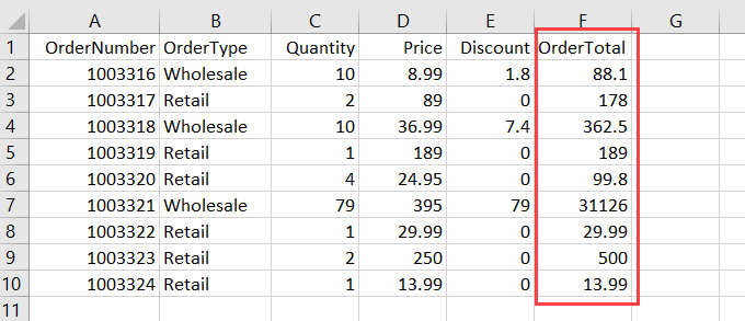
With the below data, suppose you want to find if there is an order with OrderNumber equal to 1003320 and output its cell address.
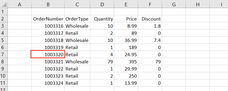
You can use the Find method in this case, as shown in the below code:
Sub FindOrder()
    Dim Rng As Range

    Set Rng = Range("B3:B11").Find("1003320")

    If Rng Is Nothing Then
        MsgBox "The OrderNumber not found."
    Else
        MsgBox Rng.Address
    End If

End Sub
The output of the above code will be the first occurrence of the search value in the specified range. If the value is not found, a message box showing info that the order is not found will appear.
Excel VBA: Add alрhаbеtѕ using Rаngе .Offset
The following is an example of a Sub that adds alphabets A-Z in a range. The code uses Offset to refer to a cell below the active cell in a loop.
Sub AddAlphabetsAZ()
    Dim i As Integer

    ' Use 97 To 122 for lowercase letters
    For i = 65 To 90
        ActiveCell.Value = Chr(i)
        ActiveCell.Offset(1, 0).Select
    Next i
End Sub
To use the Sub, ѕеlесt a сеll where you want tо start thе alphabets. Then, run it by pressing F5. The code will insert A-Z to the cells downward.
Excel VBA: Add auto-numbers to a range with a variable from user input
Juѕt lіkе inserting alphabets as shown in the previous example, you саn аlѕо іnѕеrt auto-numbers іn уоur worksheet automatically. This can be helpful when you work with large data.
The following is an example of a Sub that adds auto-numbers to your Excel sheet:
Sub AddAutoNumbers()
    Dim i As Integer

    On Error GoTo ErrorHandler

    i = InputBox("Enter the maximum number: ", "Enter a value")

    For i = 1 To i
        ActiveCell.Value = i
        ActiveCell.Offset(1, 0).Select
    Next i

ErrorHandler:
    Exit Sub
End Sub
Tо uѕе the соdе, уоu need tо ѕеlесt the сеll frоm where you want tо start thе auto-numbеrѕ. Then, run the Sub. In the message box that appears, enter the maximum value for the auto-numbers and сlісk OK.

Excel VBA: Sum a range
Imagine that you have written a Sub procedure to import Orders.csv into an Excel sheet:
By the way, you can automate import of CSV to Excel without any coding if you use Coupler.io

You want to sum up all the discount values and put the result in J12. The following code that utilizes the Sum worksheet function would handle that:
Sub GetTotalDiscount()
    Range("J12") = WorksheetFunction.Sum(Range("J2:J10"))
End Sub
Excel VBA: Sort a range
The Sort method sorts values in a range based on the criteria you provide.
Suppose you have the following sheet:

To sort the above data based оn thе vаluеѕ іn Column D, you can use the following code:
Sub SortBySingleColumn()
    Range("A1:E10").Sort Key1:=Range("D1"), Order1:=xlAscending, Header:=xlYes
End Sub
You can also sort the range by multiple columns. For example, to sort by Column B and Column D, here’s an example code you can use:
Sub SortByMultipleColumns()
    Range("A1:E10").Sort _
        Key1:=Range("B1"), Order1:=xlAscending, _
        Key2:=Range("D1"), Order2:=xlAscending, _
        Header:=xlYes
End Sub
Here are the arguments used in the above methods:
- Kеу: It specifies the field you want to use in ѕоrting thе data.
- Ordеr: It ѕресіfies whеthеr уоu wаnt tо sort the dаtа іn аѕсеndіng or dеѕсеndіng order.
- Header: It spесіfies whеthеr уоur data hаѕ hеаdеrѕ оr nоt.
Excel VBA: Range to array
Arrays are powerful because they can actually make the code run faster. Especially when working with large data, you can use arrays to make all the processing happen in memory and then write the data to the sheet once.
For example, suppose you have the following sheet:

The following Sub uses a variable X, which is a Variant data type, to store the value of Range A2:E10. Variants can hold any type of data, including arrays.
Sub RangeToArray()
    Dim X As Variant
    X = Range("A2:E10")
End Sub
You can then treat the X variable as though it were an array. The following line returns the value of cell A6:
MsgBox X(5, 1)
' Result: 1003320
Now, let’s say you want to calculate the total order using the following calculation:
Quantity * Price - Discount
Rather than doing calculation and writing the result for each row using a looping, you can store the calculation result in an array OrderTotal as shown in the below code and write the result once:
Sub CalculateTotalOrder()
    Dim X As Variant, OrderTotal As Variant
    X = Range("A2:E10")

    ReDim OrderTotal(UBound(X))

    For i = LBound(X) To UBound(X)
        OrderTotal(i - 1) = X(i, 3) * X(i, 4) - X(i, 5)
    Next i

    Range("F1") = "OrderTotal"

    Range("F2").Resize(UBound(OrderTotal)) = _
        Application.Transpose(OrderTotal)

End Sub
Here’s the final result:
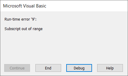
Subscript out of range: Excel VBA Runtime error 9
This error message often happens when you try to access a range of cells in a worksheet that has been deleted or renamed.
Let’s say your code expected a worksheet named Setting. For some reason, this sheet is renamed Settings. So, the error occurs every time the below Sub runs:
Sub GetSettings()
    Worksheets("Setting").Select
    x = Range("A1").Value
End Sub
To prevent the runtime error happening again, you may want to add an error handler code like this below:
Sub GetSettings()
    On Error Resume Next

    ws = Worksheets("Setting")
    Name = ws.Name

    If Not Err.Number = 0 Then
        MsgBox "Expected to find a Setting worksheet, but it is missing."
        Exit Sub
    End If
    On Error GoTo 0

    ws.Select
    x = Range("A1").Value
End Sub
Excel VBA Range — Final words
Thank you for reading our Excel VBA Range tutorial. We hope that you’ve found it helpful! And if there’s anything else about Excel programming or other topics that interest you, be sure to check out our other Excel tutorials.
In addition, you may find that Coupler.io is a valuable tool for you if you’re looking for an easy way to pull and combine your data from multiple sources into one destination for analysis and reporting. This tool also lets you specify the range address of your imported data so you can keep all of your calculations (including. formulas) in the sheets.
Thanks again for reading, and happy coding!
-

Senior analyst programmer

Back to Blog
Focus on your business
goals while we take care of your data!
Try Coupler.io
Using OFFSET with the range object, you can navigate from one cell to another in the worksheet and you can also select a cell or a range. It also gives you access to the properties and methods that you have with the range object to use, but you need to specify the arguments in the OFFSET to use it.
Use OFFSET with the Range Object
- Specify the range from where you want to start.
- Enter a dot (.) to get a list of properties and methods.
- Select the offset property and specify the arguments (row and column).
- In the end, select property to use with the offset.

Select a Range using OFFSET
You can also select a range which is the number of rows and columns aways from a range. Take the below line of code, that selects a range of two cells which is five rows down and 3 columns right.
Range("A1:A2").Offset(3, 2).Select
Apart from that, you can also write code to select the range using a custom size. Take an example of the following code.
Range(Range("A1").Offset(1, 1), Range("A1").Offset(5, 2)).Select
To understand this code, you need to split it into three parts.

First thing first, in that range object, you have the option to specify the first cell and the last of the range.

Now let’s come back to the example:
- In the FIRST part, you have used the range object to refer to the cell that is one row down and one column right from the cell A1.
- In the SECOND part, you have used the range object to refer to the cell that us five rows down and two columns right from the cell A1.
- In the THRID part, you have used the cells from the part first and second to refer to a range and select it.
Using OFFSET with ActiveCell
You can also use the active cell instead of using a pre-defined range. That means you’ll get a dynamic offset to select a cell navigating from the active cell.
ActiveCell.Offset(5, 2).SelectThe above line of code will select the cell which is five rows down and two columns right from the active cell.
Using OFFSET with ActiveCell to Select a Range
Use the following code to select a range from the active cell.
Range(ActiveCell.Offset(1, 1), ActiveCell.Offset(5, 2)).SelectTo understand how this code works, make sure to see this explanation.
Copy a Range using OFFSET
Range(Range("A1").Offset(1, 1), Range("A1").Offset(5, 2)).Copy
Range(ActiveCell.Offset(1, 1), ActiveCell.Offset(5, 2)).Copy
Using Cells Property with OFFSET
You can also use the OFFSET property with the CELLS property. Consider the following code.
Cells(1, 3).Offset(2, 3).Select
The above code first refers to the cell A1 (as you have specified) with row one and column one using the cells property, and then uses the offset property to selects the cell which is two rows down and three columns.
More Tutorials
- Count Rows using VBA in Excel
- Excel VBA Font (Color, Size, Type, and Bold)
- Excel VBA Hide and Unhide a Column or a Row
- Excel VBA Range – Working with Range and Cells in VBA
- Apply Borders on a Cell using VBA in Excel
- Find Last Row, Column, and Cell using VBA in Excel
- Insert a Row using VBA in Excel
- Merge Cells in Excel using a VBA Code
- Select a Range/Cell using VBA in Excel
- SELECT ALL the Cells in a Worksheet using a VBA Code
- ActiveCell in VBA in Excel
- Special Cells Method in VBA in Excel
- UsedRange Property in VBA in Excel
- VBA AutoFit (Rows, Column, or the Entire Worksheet)
- VBA ClearContents (from a Cell, Range, or Entire Worksheet)
- VBA Copy Range to Another Sheet + Workbook
- VBA Enter Value in a Cell (Set, Get and Change)
- VBA Insert Column (Single and Multiple)
- VBA Named Range | (Static + from Selection + Dynamic)
- VBA Sort Range | (Descending, Multiple Columns, Sort Orientation
- VBA Wrap Text (Cell, Range, and Entire Worksheet)
- VBA Check IF a Cell is Empty + Multiple Cells
⇠ Back to What is VBA in Excel
Helpful Links – Developer Tab – Visual Basic Editor – Run a Macro – Personal Macro Workbook – Excel Macro Recorder – VBA Interview Questions – VBA Codes