
В этом учебном материале по Excel мы рассмотрим примеры того как рассчитать площадь трапеции

Общая формула
= (a + b) / 2 * h
Описание
Чтобы вычислить площадь трапеции в Excel, вы можете использовать стандартную формулу, адаптированную с помощью математических операторов Excel. В показанном примере формула в E5, скопированная ниже, имеет следующий вид:
которая вычисляет площадь трапеции с учетом длины стороны a в столбце B, длины стороны b в столбце C и высоты h в столбце D.
Пояснение
В геометрии площадь трапеции определяется по следующей формуле:

где a — длина стороны a, b — длина стороны b, а h — высота, измеренная под прямым углом к основанию.
В Excel эту же формулу можно представить так:
Так, например, чтобы вычислить площадь трапеции, где a равно 3, b равно 5, а h равно 2, вы можете использовать следующую формулу:
|
= (5 + 3) / 2 * 2 Результат: 8 |
В показанном примере цель состоит в том, чтобы вычислить площадь для десяти трапеций, где a — из столбца B, b — в столбце C, а h — из столбца D.
Формула в E5:
Поскольку эта формула копируется в таблицу, она вычисляет разные площади в каждой новой строке.
См. также:
- как рассчитать площадь треугольника
- как рассчитать площадь параллелограмма
- как рассчитать площадь круга

Общая формула
=(a+b)/2*h
Резюме
Чтобы вычислить площадь трапеции в Excel, вы можете использовать стандартную формулу, адаптированную для математических операторов Excel. В показанном примере формула в E5, скопированная ниже, имеет следующий вид:
=(B5+C5)/2*D5
который вычисляет площадь трапеции с учетом длины стороны a в столбце B, длины стороны b в столбце C и высоты ( h ) в столбце D.
Объяснение
В геометрии площадь, ограниченная трапецией, определяется по этой формуле:
где a — длина стороны a, b — длина стороны b, а h — высота, измеренная под прямым углом к основанию. В Excel эту же формулу можно представить так:
=(a+b)/2*h
Так, например, чтобы вычислить площадь трапеции, где a равно 3, b равно 5 и h равно 2, вы можете использовать следующую формулу:
=(5+3)/2*2 // returns 8
В показанном примере цель состоит в том, чтобы вычислить площадь для одиннадцати трапеций, где a — из столбца B, b — из столбца C, а h — из столбца D. Формула в E5:
=(B5+C5)/2*D5
Поскольку эта формула копируется в таблицу, она вычисляет разные области в каждой новой строке.
Примечание. Скобки в этой формуле являются необязательными и предназначены только для удобства чтения. В порядке операций Excel умножение будет выполняться перед делением, поэтому скобки не нужны.
-
Практическая работа №9 – Практические задачи
Задание 1. Задачи (5 баллов)
Задание 1. Задачи
1.1. Создать файл Excel, который будет вычислять площадь трапеции по формуле
![]()
где a, b – основания тропеции, h – высота. Пересчет должен происходить автоматически при изменении сторон и высоты в отдельных ячейках пользователем.
1.2. Создать файл Excel, который будет вычислять столбец таблицы умножения на любое число. Пересчет должен происходить автоматически при изменении этого числа в отдельной ячейке пользователем.
1.3. Создать файл Excel, который будет вычислять первые 10 степеней числа. Пересчет должен происходить автоматически при изменении этого числа в отдельной ячейке пользователем. Примечание: воспользуйтесь в формуле знаком ^n, который означает возведение в n-ю степень.
1.4. Создать файл Excel, который будет число в гигабайтах переводить в мегабайты, килобайты, байты и биты. Пересчет должен происходить автоматически при изменении количества гигабайт в отдельной ячейке пользователем. Примечание: в одном гигабайте 1024 мегабайта, в одном мегабайте 1024 килобайта, в одном килобайте 1024 байта, в одном байте 8 бит.
1.5. Создать файл Excel, который будет число в битах переводить байты, килобайты, мегабайты и гигабайты. Пересчет должен происходить автоматически при изменении количества бит в отдельной ячейке пользователем. Примечание: в одном гигабайте 1024 мегабайта, в одном мегабайте 1024 килобайта, в одном килобайте 1024 байта, в одном байте 8 бит.
1.6. Создать файл Excel, который будет вычислять 10, 35, 52, 64 и 87 процентов от любого числа. Пересчет должен происходить автоматически при изменении этого числа в отдельной ячейке пользователем. Примечание: чтобы посчитать процент от числа, нужно умножить число на этот процент и разделить полученное число на 100.
Summary
To calculate the area of a trapezoid in Excel, you can use a standard formula, adapted to for Excel’s math operators. In the example shown, the formula in E5, copied down, is:
=(B5+C5)/2*D5
which calculates the area of a trapezoid given the length of side a in column B, the length of side b in column C, and the height (h) in column D.
Generic formula
Explanation
In geometry, the area enclosed by a trapezoid is defined by this formula:
where a is the length of side a, b is the length of side b, and h is the height, measured at a right angle to the base. In Excel, the same formula can be represented like this:
=(a+b)/2*h
So, for example, to calculate the area of a trapezoid where a is 3, b is 5, and h is 2, you can use a formula like this:
=(5+3)/2*2 // returns 8
In the example shown, the goal is to calculate the area for eleven trapezoids where a comes from column B, b is in column C, and h comes from column D. The formula in E5 is:
=(B5+C5)/2*D5
As this formula is copied down the table, it calculates a different area at each new row.
Note: The parentheses in this formula are optional and for readability only. In Excel’s order of operations, multiplication will occur before division, so the parentheses are unnecessary.

Author![]()
Dave Bruns
Hi — I’m Dave Bruns, and I run Exceljet with my wife, Lisa. Our goal is to help you work faster in Excel. We create short videos, and clear examples of formulas, functions, pivot tables, conditional formatting, and charts.
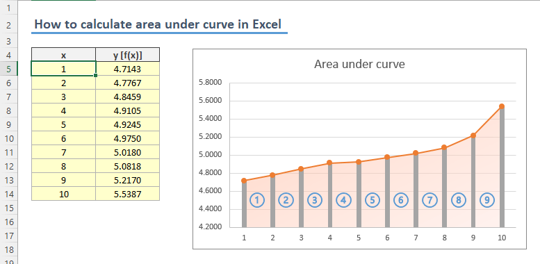
In this guide, we’re going to show you how to calculate area under curve in Excel.
Download Workbook
Unfortunately, there isn’t a single function or feature that can calculate area under curve in Excel. You can still rely on integrals to calculate area. On the other hand, Excel can help us with a simpler approach as well.
Calculating area under curve by trapezoidal rule
The trapezoidal rule is a technique for approximating the region under the graph as a trapezoid and calculating its area. The rule can be depicted as following:

Because we have the data which generates the chart, we can easily transform the above formula into a format that Excel can calculate each trapezoid’s area individually.
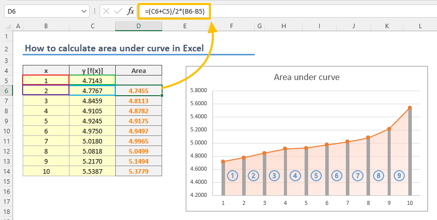
- Start by inserting a helper column in your data set. Adjacent columns will ease copying of the formula. This column will calculate the area of each trapezoid between data points (x).

- Enter the area formula starting from the second row. The formula will refer the data points in the same (k) and the previous row (k-1).
=(C6+C5)/2*(B6-B5)
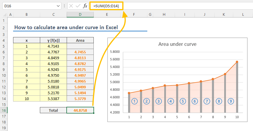
- Sum all area values to find the total area under the curve.


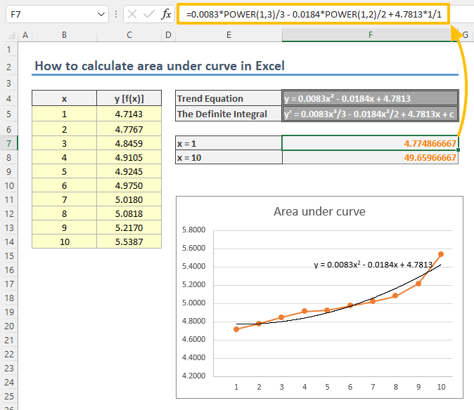
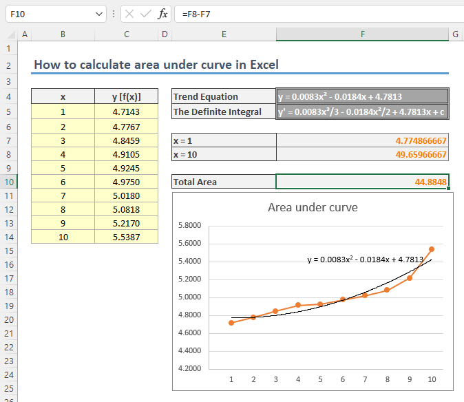
Using Chart Trendline
An alternative approach is to use the equation of the plotted curve. Excel can plot a trendline based on your values and generate an equation for the trendline as well.
- Select your chart.
- Either use the Chart Elements button (plus button at the top-right) or Add Chart Element command in the Chart Design tab of the Ribbon to select More Options item.

- More Options command adds a trendline and opens the properties pane at the rights side. Under Trendline Options, select Polynomial type and check the Display Equation on chart property.

- Next step is the trickiest of this article if you are not familiar with integrals. Briefly, you need the convert the equation to its definite integral and calculate the minimum and maximum values through the definite integral. The difference between the two results will give the area under curve.
You need to increase the power of each x value by 1 and divide it by the increased power value. For example, x² becomes x³/3. According to this our formula will be the following:
- Next step is to calculate the definite integral values for the smallest and the largest x. You can omit the c values since the subtracting operations nullifies them. These are 1 and 10 in our example:

- Final step is to find the difference to calculate the area under curve.


Remarks
As you can realize there is a small difference between the results of each approach. Since each approach returns an approximate value, it would be better to use both and compare.
If you are a Microsoft 365 subscriber, you can use either the LET or the LAMBDA functions to simplify the use of the definite integral formula multiple times.