
Return the number of columns in a given array or reference
How to Get Excel Last Value in Column
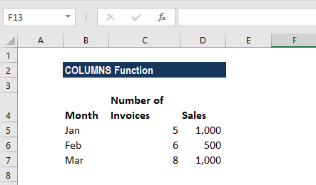
The COLUMNS Function[1] in Excel is an Excel Lookup/Reference function. It is useful for looking up and providing the number of columns in a given reference or array. The COLUMNS function, after specifying an Excel range, will return the number of columns that are contained within that range.
Formula
=COLUMNS(array)
The COLUMNS function in Excel includes only one argument – array. The array argument is a required argument. It is the reference to a range of cells or an array or array formula for which we want the number of columns. The function returns a numerical value.
How to use the COLUMNS Function in Excel?
It is a built-in function that can be used as a worksheet function in Excel. To understand the uses of this function, let’s consider a few examples:
Example 1
Let’s see how this function works when we provide the following references:
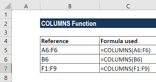
Suppose we wish to find out the number of columns in a range. The most basic formula used is = COLUMNS(rng).
In the first reference above, we used the COLUMNS function to get the number of columns from range A6:F6. We got the result as 6 as shown in the screenshot below:
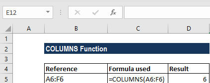
So, this function counted the number of columns and returned a numerical value as the result.
When we gave the cell reference B6, it returned the result of 1, as only one reference was given.
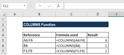
Lastly, when we provided the formula F1:F9, it counted the number of columns as 1 and the function returned the result accordingly.
Thus, in this function, “array” can be an array, an array formula, or a reference to a single contiguous group of cells.
COLUMNS Function – Example 2
Using Columns with other formulas: If we wish to get the address of the first cell in a named range, we can use the ADDRESS function together with the ROW and COLUMN functions. The formula to be used is below:
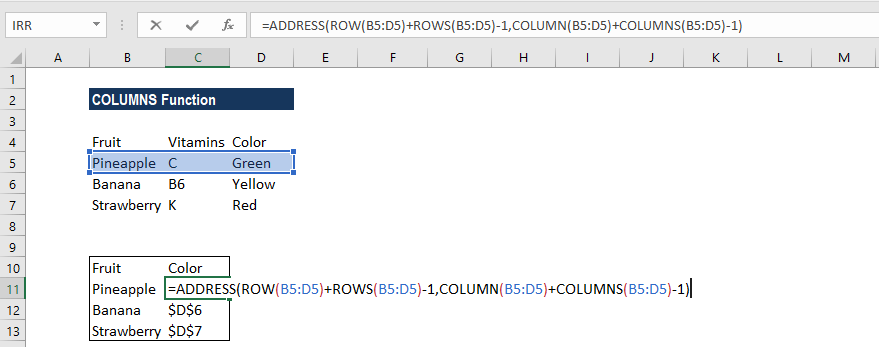
What happens in this formula is that the ADDRESS function builds an address based on a row and column number. Then, we use the ROW function to generate a list of row numbers, which are then shifted by adding ROWS(B5:D5)-1, so that the first item in the array is the last row number:
ROW(B5:D5)+ROWS(B5:D5)-1
We do the same for COLUMN and COLUMNS: COLUMN(B5:D5)+COLUMNS(B5:D5)-1
What happens is that the ADDRESS function now collects and returns an array of addresses. If we enter the formula in a single cell, we just get the item from the array, which is the address corresponding to the last cell in a range.
COLUMNS Function – Example 3
Now let’s see how to find out the last column in a range. The data given is as follows:
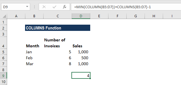
The formula used is =MIN(COLUMN(A3:C5))+COLUMNS(A3:C5)-1
Using the formula above, we can get the last column that is in a range with a formula based on the COLUMN function.
When we give a single cell as a reference, the COLUMN function will return the column number for that particular reference. However, when we give a range that contains multiple columns, the COLUMN function will return an array that contains all column numbers for the given range.
If we wish to get only the first column number, we can use the MIN function to extract just the first column number, which will be the lowest number in the array.
Once we get the first column, we can just add the total columns in the range and subtract 1, to get the last column number.
The result is shown below:
For a very large number of ranges, we can use the INDEX function instead of the MIN function. The formula would be:
=COLUMN(INDEX(range,1,1))+COLUMNS(range)-1
Click here to download the sample Excel file
Additional Resources
Thanks for reading CFI’s guide to important Excel functions! By taking the time to learn and master these functions, you’ll significantly speed up your financial analysis. To learn more, check out these additional CFI resources:
- Excel Functions for Finance
- Advanced Excel Formulas Course
- Advanced Excel Formulas You Must Know
- Excel Shortcuts for PC and Mac
- See all Excel resources
Article Sources
- COLUMNS Function
How to find the last column in a row that has data. This includes selecting that column or a cell in it, returning the column number, and getting data from that column.
Sections:
Find the Last Column with Data
Select the Last Cell
Select the Entire Column
Get the Number of the Last Column
Get the Data from the Last Column
Notes
Find the Last Column with Data
Cells(1, Columns.Count).End(xlToLeft)
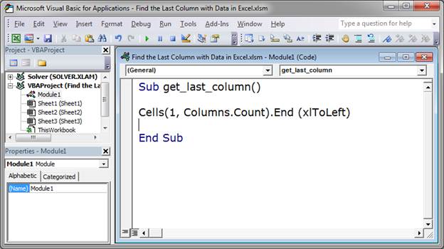
All you have to change to make this work for you is the 1.
This is the basic method that you use to return the last cell in a row that has data. That means that the cell will be in the last column that has data.
The 1 in the above code is the number of the row that you want to use when searching for the last column that has data. Currently, this code looks in row 1 and finds the last column in row 1 that has data. Change this to any number you want.
This doesn’t seem very useful right now, but, in practice, it is often used within a loop that goes through a list of rows and you can then set this code to find the last column of data for each row without having to manually change this number.
Columns.Count puts the total number of columns in for that argument of the Cells() function. This tells Excel to go to the very last cell in the row, all the way to the right.
Then, End(xlToLeft) tells Excel to go to the left from that last cell until it hits a cell with data in it.
This basic format is also used to find the last row in a column.
Now, let’s look at how to get useful information from this code.
Select the Last Cell
The first thing that you might want to do is to select the cell that has data in the last column of a row.
Cells(1, Columns.Count).End(xlToLeft).Select
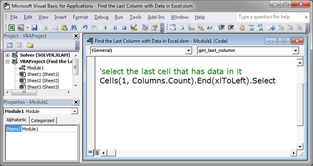
Select is what selects that last cell in the row that has data.
This is exactly the same as the first piece of code except we added Select to the end of it.
1 is the row that is being checked.
Select the Entire Column
This selects the entire column where the last cell with data is found within a particular row.
Cells(1, Columns.Count).End(xlToLeft).EntireColumn.Select
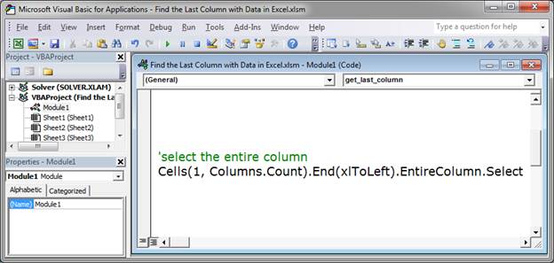
EntireColumn is added to the base code and that is what references, well, the entire column.
Select is added to the end of EntireColumn and that is what does the actual «selecting» of the column.
1 is the row that is being checked.
Get the Number of the Last Column
Let’s get the number of the last column with data. This makes it easier to do things with that column, such as move one to the right of it to find the next empty cell in a row.
Cells(1, Columns.Count).End(xlToLeft).Column
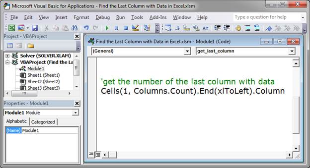
Column is appended to the original code in order to give us the number of the column that contains the last piece of data in a row.
This is rather useless on its own though, so let’s put it into a variable so it can be used throughout the macro.
last_col = Cells(1, Columns.Count).End(xlToLeft).Column
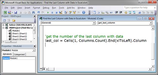
The number of the last column is now stored in the variable last_col and you can now use that variable to reference this number.
1 is the row that is being checked.
Get the Data from the Last Column
Return any data contained in the cell in the last column.
Cells(1, Columns.Count).End(xlToLeft).Value
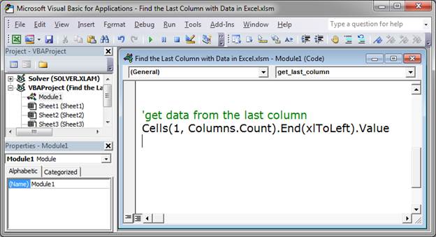
Value is added to the end of the base code in order to get the contents of the cell.
This is rather useless in its current form so let’s put it into a variable.
cell_value = Cells(1, Columns.Count).End(xlToLeft).Value
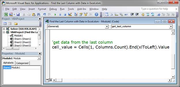
Now, the variable cell_value will contain anything that is in the last cell in the row.
1 is the row that is being checked.
Notes
The basic format for finding the last cell that has data in a row is the same and is the most important part to remember. Each piece of information that we want to get from that last cell simply requires one or two things to be added to the end of that base code.
Download the attached file to work with these examples in Excel.
Similar Content on TeachExcel
Get the Last Row using VBA in Excel
Tutorial:
(file used in the video above)
How to find the last row of data using a Macro/VBA in Exce…
Next Empty Row Trick in Excel VBA & Macros
Tutorial:
A simple way to find the next completely empty row in Excel using VBA/Macros, even if som…
How to Add a New Line to a Message Box (MsgBox) in Excel VBA Macros
Tutorial: I’ll show you how to create a message box popup window in Excel that contains text on mult…
Loop Through an Array in Excel VBA Macros
Tutorial:
I’ll show you how to loop through an array in VBA and macros in Excel. This is a fairly…
Filter Data in Excel to Show Only the Top X Percent of that Data Set — AutoFilter
Macro: This Excel macro filters a set of data in Excel and displays only the top X percent of tha…
Sort Data Left to Right in Excel
Tutorial: How to sort columns of data in Excel. This is the same as sorting left to right.
This wi…
Subscribe for Weekly Tutorials
BONUS: subscribe now to download our Top Tutorials Ebook!
Была в сети 15.04.2023 10:16

Руденко Наталия Владимировна
учитель физики и информатики
32 года
![]() 5 777
5 777
![]() 5 337
5 337 ![]()
04.12.2017 22:20

«Назначение и интерфейс MS Excel»
Выполнив задания этой темы, вы:
1. Научитесь запускать электронные таблицы;
2. Закрепите основные понятия: ячейка, строка, столбец, адрес ячейки;
3. Узнаете как вводить данные в ячейку и редактировать строку формул;
5. Как выделять целиком строки, столбец, несколько ячеек, расположенных рядом и таблицу целиком.
Задание: Познакомиться практически с основными элементами окна MS Excel.

Технология выполнения задания:
- Запустите программу Microsoft Excel. Внимательно рассмотрите окно программы.
Документы, которые создаются с помощью EXCEL , называются рабочими книгами и имеют расширение . XLS . Новая рабочая книга имеет три рабочих листа, которые называются ЛИСТ1, ЛИСТ2 и ЛИСТ3. Эти названия указаны на ярлычках листов в нижней части экрана. Для перехода на другой лист нужно щелкнуть на названии этого листа.
Действия с рабочими листами:
- Переименование рабочего листа. Установить указатель мыши на корешок рабочего листа и два раза щелкнуть левой клавишей или вызвать контекстное меню и выбрать команду Переименовать. Задайте название листа «ТРЕНИРОВКА»
- Вставка рабочего листа. Выделить ярлычок листа «Лист 2», перед которым нужно вставить новый лист, и с помощью контекстного меню вставьте новый лист и дайте название «Проба» .
- Удаление рабочего листа. Выделить ярлычок листа «Лист 2», и с помощью контекстного меню удалите.
Ячейки и диапазоны ячеек.
Рабочее поле состоит из строк и столбцов. Строки нумеруются числами от 1 до 65536. Столбцы обозначаются латинскими буквами: А, В, С, …, АА, АВ, … , IV , всего – 256. На пересечении строки и столбца находится ячейка. Каждая ячейка имеет свой адрес: имя столбца и номер строки, на пересечении которых она находится. Например, А1, СВ234, Р55.
Для работы с несколькими ячейками их удобно объединять их в «диапазоны».
Диапазон – это ячейки, расположенные в виде прямоугольника. Например, А3, А4, А5, В3, В4, В5. Для записи диапазона используется «:»: А3:В5
8:20 – все ячейки в строках с 8 по 20.
А:А – все ячейки в столбце А.
Н:Р – все ячейки в столбцах с Н по Р.
В адрес ячейки можно включать имя рабочего листа: Лист8!А3:В6.
2. Выделение ячеек в Excel
|
Что выделяем |
Действия |
|
Одну ячейку |
Щелчок на ней или перемещаем выделения клавишами со стрелками. |
|
Строку |
Щелчок на номере строки. |
|
Столбец |
Щелчок на имени столбца. |
|
Диапазон ячеек |
Протянуть указатель мыши от левого верхнего угла диапазона к правому нижнему. |
|
Несколько диапазонов |
Выделить первый, нажать SCHIFT + F 8, выделить следующий. |
|
Всю таблицу |
Щелчок на кнопке «Выделить все» (пустая кнопка слева от имен столбцов) |
Можно изменять ширину столбцов и высоту строк перетаскиванием границ между ними.
Воспользуйтесь полосами прокрутки для того, чтобы определить сколько строк имеет таблица и каково имя последнего столбца.
Внимание!!! Чтобы достичь быстро конца таблицы по горизонтали или вертикали, необходимо нажать комбинации клавиш: Ctrl+→ — конец столбцов или Ctrl+↓ — конец строк. Быстрый возврат в начало таблицы — Ctrl+Home.
В ячейке А3 Укажите адрес последнего столбца таблицы.
Сколько строк содержится в таблице? Укажите адрес последней строки в ячейке B3.
3. В EXCEL можно вводить следующие типы данных:
- Числа.
- Текст (например, заголовки и поясняющий материал).
- Функции (например, сумма, синус, корень).
- Формулы.
Данные вводятся в ячейки. Для ввода данных нужную ячейку необходимо выделить. Существует два способа ввода данных:
- Просто щелкнуть в ячейке и напечатать нужные данные.
- Щелкнуть в ячейке и в строке формул и ввести данные в строку формул.
Нажать ENTER .
Введите в ячейку N35 свое имя, выровняйте его в ячейке по центру и примените начертание полужирное.
Введите в ячейку С5 текущий год, используя строку формул.
4. Изменение данных.
- Выделить ячейку и нажать F 2 и изменить данные.
- Выделить ячейку e щелкнуть в строке формул и изменить данные там.
Для изменения формул можно использовать только второй способ.
Измените данные в ячейке N35, добавьте свою фамилию. используя любой из способов.
5. Ввод формул.
Формула – это арифметическое или логическое выражение, по которому производятся расчеты в таблице. Формулы состоят из ссылок на ячейки, знаков операций и функций. Ms EXCEL располагает очень большим набором встроенных функций. С их помощью можно вычислять сумму или среднее арифметическое значений из некоторого диапазона ячеек, вычислять проценты по вкладам и т. д.
Ввод формул всегда начинается со знака равенства. После ввода формулы в соответствующей ячейке появляется результат вычисления, а саму формулу можно увидеть в строке формул.
|
Оператор |
Действие |
Примеры |
|
+ |
Сложение |
= А1+В1 |
|
— |
Вычитание |
= А1 — В2 |
|
* |
Умножение |
= В3*С12 |
|
/ |
Деление |
= А1 / В5 |
|
^ |
Возведение в степень |
= А4 ^3 |
|
=, <,>,<=,>=,<> |
Знаки отношений |
=А2 <D2 |
В формулах можно использовать скобки для изменения порядка действий.
- Автозаполнение.
Очень удобным средством, которое используется только в MS EXCEL , является автозаполнение смежных ячеек. К примеру, необходимо в столбец или строку ввести названия месяцев года. Это можно сделать вручную. Но есть гораздо более удобный способ:
- Введите в первую ячейку нужный месяц, например январь.
- Выделите эту ячейку. В правом нижнем углу рамки выделения находится маленький квадратик – маркер заполнения.
- Подведите указатель мыши к маркеру заполнения (он примет вид крестика), удерживая нажатой левую кнопку мыши, протяните маркер в нужном направлении. При этом радом с рамкой будет видно текущее значение ячейки.
Если необходимо заполнить какой-то числовой ряд, то нужно в соседние две ячейки ввести два первых числа (например, в А4 ввести 1, а в В4 – 2), выделить эти две ячейки и протянуть за маркер область выделения до нужных размеров.
Просмотр содержимого документа
«Практическая работа 1 «Назначение и интерфейс MS Excel»»
Рекомендуем курсы ПК и ППК для учителей
Похожие файлы
Excel для Microsoft 365 Excel для Microsoft 365 для Mac Excel для Интернета Еще…Меньше
Windows: 2208 (сборка 15601)
Mac: 16.65 (сборка 220911)
Веб: представлено 15 сентября 2022
г.
iOS: 2.65 (сборка 220905)
Android: 16.0.15629
Возвращает указанные столбцы из массива.
Синтаксис
=ВЫБОРСТОЛБЦ(массив; номер_столбца1; [номер_столбца2];…)
Аргументы функции ВЫБОРСТОЛБЦ описаны ниже.
-
массив Массив, содержащий столбцы, которые должны быть возвращены в новом массиве. Обязательный.
-
номер_столбца1 Первый возвращаемый столбец. Обязательный.
-
номер_столбца2 Дополнительные столбцы, которые необходимо вернуть. Необязательный.
Ошибки
Excel возвращает ошибку #ЗНАЧ, если абсолютное значение любого из аргументов «номер_столбца» является нулем или превышает количество столбцов в массиве.
Примеры
Скопируйте данные примера из таблицы ниже и вставьте их в ячейку A1 нового листа Excel. При необходимости измените ширину столбцов, чтобы видеть все данные.
Возвращает массив столбцов 1, 3, 5 и снова 1 из массива в диапазоне A2:E7.
|
Данные |
|||||
|
1 |
2 |
3 |
4 |
5 |
|
|
6 |
7 |
8 |
9 |
10 |
|
|
11 |
12 |
13 |
14 |
15 |
|
|
16 |
17 |
18 |
19 |
20 |
|
|
21 |
22 |
23 |
24 |
25 |
|
|
26 |
27 |
28 |
29 |
30 |
|
|
Формулы |
|||||
|
=ВЫБОРСТОЛБЦ(A2:E7,1,3,5,1) |
Возвращает массив из двух последних столбцов из массива в диапазоне A2:D7 в следующем порядке: столбец три, а затем столбец четыре.
|
Данные |
|||
|
1 |
2 |
13 |
14 |
|
3 |
4 |
15 |
16 |
|
5 |
6 |
17 |
18 |
|
7 |
8 |
19 |
20 |
|
9 |
10 |
21 |
22 |
|
11 |
12 |
23 |
24 |
|
Формулы |
|||
|
=ВЫБОРСТОЛБЦ(A2:D7;3;4) |
Возвращает массив из двух последних столбцов из массива в диапазоне A2:D7 в следующем порядке: столбец четыре, а затем столбец три.
|
Данные |
|||
|
1 |
2 |
13 |
14 |
|
3 |
4 |
15 |
16 |
|
5 |
6 |
17 |
18 |
|
7 |
8 |
19 |
20 |
|
9 |
10 |
21 |
22 |
|
11 |
12 |
23 |
24 |
|
Формулы |
|||
|
=ВЫБОРСТОЛБЦ(A2:D7,-1,-2) |
См. также
Использование формул массива: рекомендации и примеры
Функция ВСТОЛБИК
Функция ГСТОЛБИК
Функция CHOOSEROWS