
Skip to content
![]()
This is a problem that occurs once a while in Excel: Some objects are not showing. Most often, images or charts are not showing. Here are the possible reasons if charts, objects or images are missing and how to get them back!
Possible reasons for missing images and charts in Excel
You had images, charts or other objects (e.g. drawing) in your Excel workbook, but now they are gone? There are basically two possibilities:
- You’ve (accidentally) deleted them?
- They are just not being displayed.
So, let’s see now how to get them back.
Reason 1: How to get images and charts back if you have deleted them
If you are sure that you have not accidentally deleted charts or images, just scroll down to reason number 2.
If you have deleted pictures, charts or objects, try these things:
- Undo (Ctrl + Z) until pictures are shown.
If you have already changed many things, you can repeat undo until the images and charts are back, copy them, redo as long as necessary and paste them. - Restore an older version of your file. Here is how to do that.
Reason 2: Simply display images within the Excel options
There is a hidden setting in Excel with says “For objects, show:”. Here you can select if you want to show all such objects. Objects are in general everything which is not inside cells. So everything from images, drawings, charts, drop-down lists, etc.
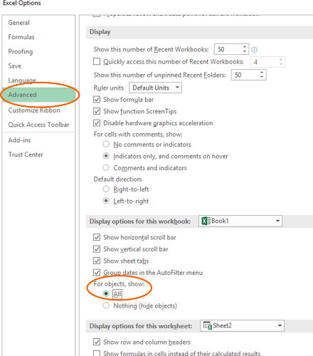
You can easily reactivate them. But it’s a little bit hidden:
- Go to File and click on Options.
- On the left side click on “Advanced”.
- Scroll down to the “Display options for this workbook:”. The last bullet point says “For objects, show:”. Set the tick at “All”.
That’s it
Image by Amanda Elizabeth from Pixabay

Henrik Schiffner is a freelance business consultant and software developer. He lives and works in Hamburg, Germany. Besides being an Excel enthusiast he loves photography and sports.
We use cookies on our website to give you the most relevant experience by remembering your preferences and repeat visits. By clicking “Accept”, you consent to the use of ALL the cookies.
.
How to Insert Pictures Into Excel Cells – Step-by-step (2023)
I bet you know how to insert pictures but do you know how to insert a picture into a cell in Excel?
It’s a fairly simple, but quite unknown method that ultimately locks the image to a cell.
Let me show you how it’s done, step-by-step💡
If you want to tag along, download my Excel sample file here.
How to insert a picture into a cell in Excel
Unlike with some other platforms, you simply can’t copy and paste a picture into an Excel cell.
But I assure you that the process to insert images isn’t difficult.
In fact, the image shown below took only 30 seconds to do.

1. Go to the Insert tab.
2. Click the Illustrations button.
3. Select Picture and choose where the image should come from.
Typically, the image is located on your computer. If that’s the case, select ‘From this device’.

4. Select the images you want to insert.
Tip: You can insert multiple images at the same time.
5. Resize the image to fit the cell and make sure to move the picture into a cell.
Pretty easy, huh?
PRO TIP: KEEP ASPECT RATIO OF IMAGE
When you resize an image in Excel the aspect ratio can get out of hand really quickly, making it look ridiculous.
To keep the aspect ratio intact, make sure to resize it by dragging the handles at the corners of the image.
Don’t drag the handles to the top, bottom, left, or right.

After resizing the images to fit the cells, there’s one problem left:
Resizing the columns or rows where the images reside does not affect the images.
Here’s what I mean:

To solve that, you have to lock the picture into a cell.
How to lock an image to a cell
For the image to resize when you resize the columns or rows, you will have to change its properties.
1. Right-click on the image and select ‘Format Picture’.

This will open the format picture pane where you can change the picture settings.
2. Click on the ‘Size and properties’ button.
3. Expand the ‘Properties’ tab and click ‘Move and size with cells’.

And that’s how you lock a picture into a cell in Excel.
Now, when you resize the cell the image is automatically resized with the cell.
If you insert multiple images, you can select them all by holding down the Shift key while left-clicking each one.
Do this before enabling ‘Move and size with cells’ from the Properties tab in the ‘Format picture pane’ and it’ll be done to all the images at once.
That’s it – What’s next?
As you can see, it’s pretty quick and easy to insert a picture into Excel cells.
The real challenge is making sure that the photo moves and resizes with the cell. Luckily, you can lock the picture into a cell to make that happen.
But to insert an image is only a small part of Microsoft Excel.
Excel can automate calculations, make decisions for you, speed up your daily work, and join data from multiple files in a few seconds.
If you want to get started with all that, you should enroll in my 30-minute free Excel training program that adapts to your Excel skill level.
Click here and sign up with your email address to get instant access to the course.
Other resources
Now that you’re inserting pictures into Excel cells, I got some other relevant resources for you.
Another way of displaying images in your Excel file is by showing them as watermarks. Read all about that here.
Also, if you care about the general look and feel of your spreadsheet, you need to know a few tricks like adding headers and footers, the format painter, and number formats.
Kasper Langmann2023-01-19T12:29:25+00:00
Page load link
Author: Oscar Cronquist Article last updated on February 14, 2023

This article explains how to hide a specific image in Excel using a shape as a button. If the user press with left mouse button ons the shape the image disappears, press with left mouse button on again and it is visible.
What’s on this page
- Insert a shape
- Insert an image
- Show/Hide an image using a VBA macro
- Where to put the code?
- Link macro to shape
- Place image next to the upper-right corner of shape
- Place image next to the upper-left corner of shape
- Place image next to the lower-left corner of shape
- Get Excel *.xlsm file
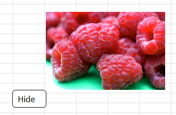
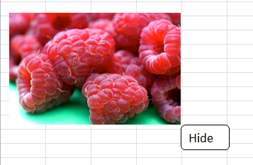
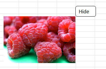
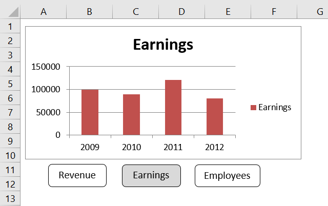
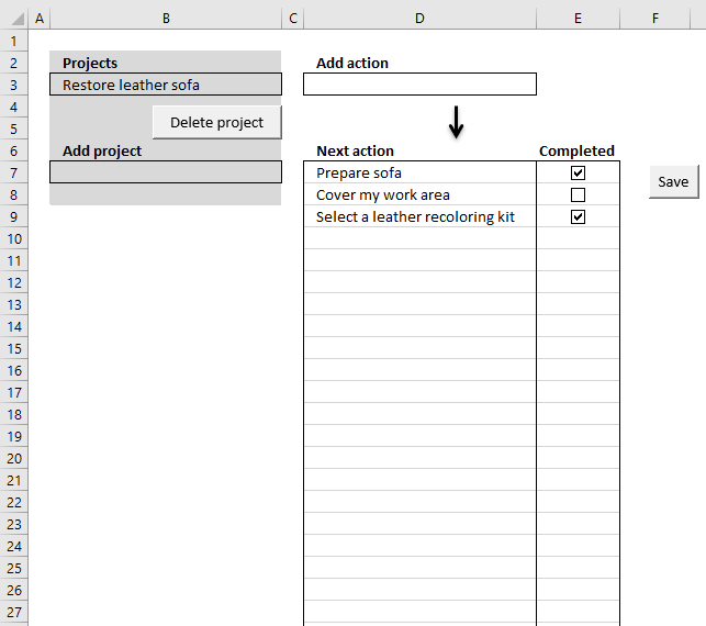
The following animated image shows when you press with left mouse button on the shape, the picture is hidden. Press with left mouse button on it again and the picture shows up. The macro changes the shape text based on the state of the image.
Move and press with left mouse button on the shape and the picture is automatically repositioned to the lower right shape corner. You can also position the picture wherever you like, I’ll show later in this post how to accomplish that.
Instructions
First, let’s create a button (shape). This time I will not use a regular button (Form Controls), I will use a shape. I chose a shape with rounded corners.
Back to top
Insert a shape

- Go to tab «Insert» on the ribbon.
- Press with left mouse button on «Shapes» button located on the ribbon. A pop-up menu appears, see image above.
- Press with mouse on a shape to select it. I chose a rounded rectangle.
- Press and hold with left mouse button on the worksheet. Drag with mouse to place and create the shape.

The image above shows a new shape. The round white circles around the shape are sizing handles.
The sizing handles indicate that the shape is selected. To select a shape simply press with left mouse button on with left mouse button on a shape and the sizing handles appear.
Press with left mouse button on anywhere outside the shape to deselect it. To move a shape press and hold with left mouse button on it and then drag with mouse to the new location.
Press and hold with left mouse button on a sizing handle, then drag with mouse to resize the shape.
Press and hold Alt key to align shape with cell grid while moving or resizing the shape.
Back to top
Insert a picture
- Copy a picture.
- Paste a picture to a worksheet.
- Select the picture to see the name. The name appears in the name bar, see image below.

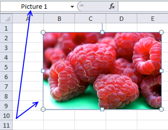
Note, you change the name of the shape using the name bar. Press with left mouse button on the text in the name bar, edit the text then press Enter.
Back to top
VBA Code
'Name macro
Sub Macro1()

'The With ... End With statement allows you to write shorter code by referring to an object only once instead of using it with each property.
With ActiveSheet.Shapes("Rounded Rectangle 4").TextFrame2.TextRange.Characters

   'Check if shape text is equal to "Hide"
   If .Text = "Hide" Then

      'Change shape text to "Show"
      .Text = "Show"

      'Hide shape
      ActiveSheet.Shapes("Picture 1").Visible = False

   'Continue here if shape is not equal to "Hide"
   Else

      'Change text to "Hide"
      .Text = "Hide"

      'The With ... End With statement allows you to write shorter code by referring to an object only once instead of using it with each property.
      With ActiveSheet.Shapes("Rounded Rectangle 4")

         'Move image named "Picture1" based to lower right corner of shape
         ActiveSheet.Shapes("Picture 1").Left = .Left + .Width
         ActiveSheet.Shapes("Picture 1").Top = .Top + .Height

         'Show image
         ActiveSheet.Shapes("Picture 1").Visible = True
      End With
    End If
End With
End Sub
Back to top
Where to put the code?
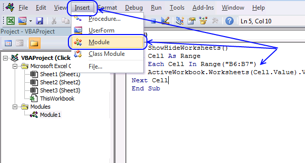
- Press Alt + F11 to start the Visual Basic Editor (VBE).
- Press with left mouse button on «Insert» on the menu, see image above.
- Press with left mouse button on «Module».
- Paste VBA code to window.
- Exit VB Editor and return to Excel.
Note, save the workbook with file extension *.xlsm (macro-enabled workbook) to keep the code attached to the workbook.
Back to top
How to assign a macro to shape

- Press with right mouse button on on the shape. A pop-up menu appears.
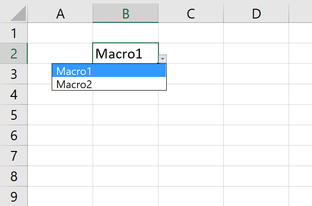
- Press with left mouse button on «Assign Macro…», see image above. A dialog box shows up.
- Select Macro1 in the list.

- Press with left mouse button on OK button to assign Macro1 to the shape.

Back to top
Positioning the picture
The following examples demonstrate how to place a picture in relation to a shape using VBA.
Place image next to the upper right corner of a shape
These VBA lines change the position of the image to the upper right corner of the shape. The picture name is «Picture 1» and the last line below makes it visible.
'The With ... End With statement allows you to write shorter code by referring to an object only once instead of using it with each property.
With ActiveSheet.Shapes("Rounded Rectangle 4")

'Place image next to the upper right corner
ActiveSheet.Shapes("Picture 1").Left = .Left + .Width
ActiveSheet.Shapes("Picture 1").Top = .Top - ActiveSheet.Shapes("Picture 1").Height

'Show image
ActiveSheet.Shapes("Picture 1").Visible = True
End With
Back to top
Place image next to the upper left corner of a shape
'The With ... End With statement allows you to write shorter code by referring to an object only once instead of using it with each property.
With ActiveSheet.Shapes("Rounded Rectangle 4")

'Place image next to the upper left corner
ActiveSheet.Shapes("Picture 1").Left = .Left - ActiveSheet.Shapes("Picture 1").Width
ActiveSheet.Shapes("Picture 1").Top = .Top - ActiveSheet.Shapes("Picture 1").Height

'Show image
ActiveSheet.Shapes("Picture 1").Visible = True
End With
Back to top
Place image next to the lower left corner of a shape
'The With ... End With statement allows you to write shorter code by referring to an object only once instead of using it with each property.
With ActiveSheet.Shapes("Rounded Rectangle 4")

'Place image next to the lower left corner
ActiveSheet.Shapes("Picture 1").Left = .Left - ActiveSheet.Shapes("Picture 1").Width
ActiveSheet.Shapes("Picture 1").Top = .Top + .Height

'Show image
ActiveSheet.Shapes("Picture 1").Visible = True
End With
Back to top
Back to top
Recommended articles
Recommended articles
Recommended articles
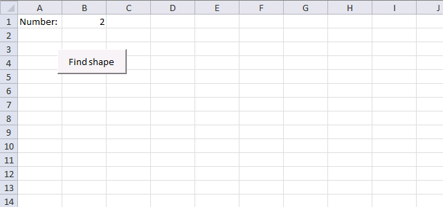
Locate a shape in a workbook
This article demonstrates how to locate a shape in Excel programmatically based on the value stored in the shape. The […]
Recommended articles
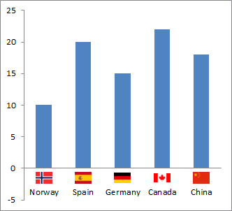
Add pictures to a chart axis
This article demonstrates how to insert pictures to a chart axis, the picture above shows a column chart with country […]
Recommended links
- VBA Code to insert, move, delete and control pictures
- Show Picture on Mouse Hover with VBA
- Showing a picture from a list of pictures
Back to top
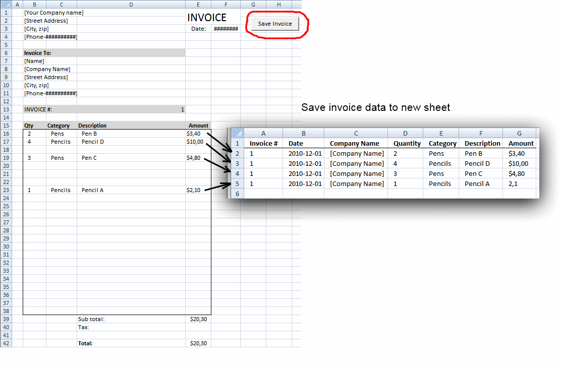
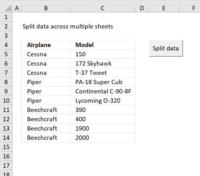
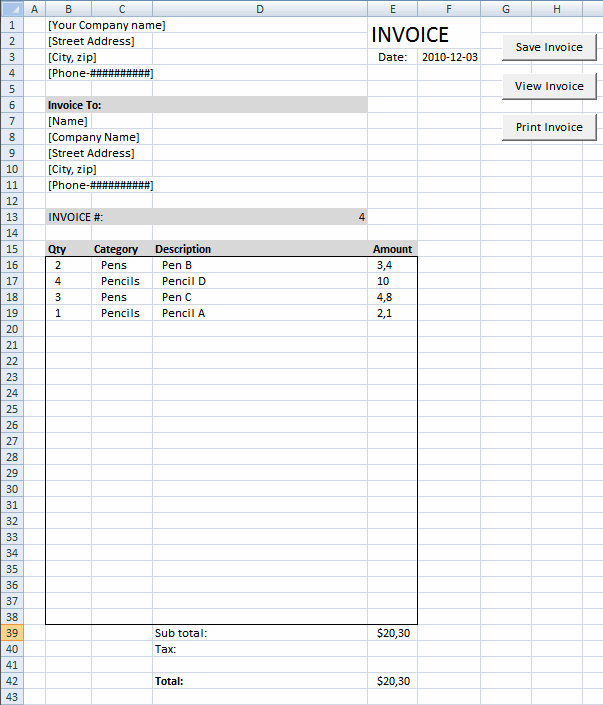
Save invoice data [VBA]
This article demonstrates a macro that copies values between sheets. I am using the invoice template workbook. This macro copies […]
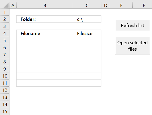
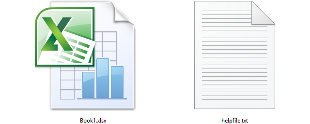
Open Excel files in a folder [VBA]
This tutorial shows you how to list excel files in a specific folder and create adjacent checkboxes, using VBA. The […]
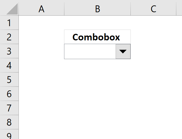
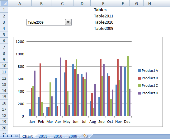
Working with COMBO BOXES [Form Controls]
This blog post demonstrates how to create, populate and change comboboxes (form control) programmatically. Form controls are not as flexible […]
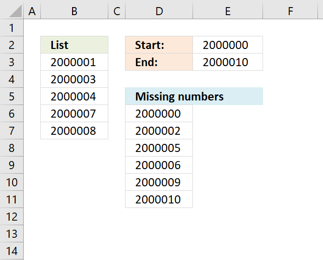
Identify missing numbers in a column
The image above shows an array formula in cell D6 that extracts missing numbers i cell range B3:B7, the lower […]
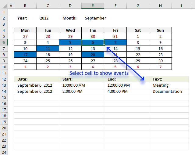
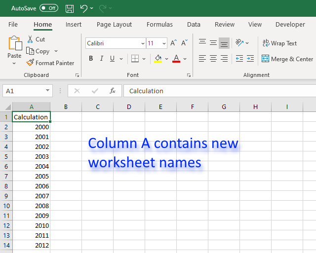
Excel calendar [VBA]
This workbook contains two worksheets, one worksheet shows a calendar and the other worksheet is used to store events. The […]
Working with FILES
In this blog article, I will demonstrate basic file copying techniques using VBA (Visual Basic for Applications). I will also […]
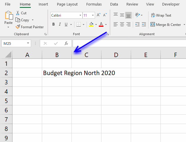
Auto resize columns as you type
Excel does not resize columns as you type by default as the image above demonstrates. You can easily resize all […]
Create a Print button [VBA]
This article describes how to create a button and place it on an Excel worksheet then assign a macro to […]
Latest updated articles.
More than 300 Excel functions with detailed information including syntax, arguments, return values, and examples for most of the functions used in Excel formulas.
More than 1300 formulas organized in subcategories.
Excel Tables simplifies your work with data, adding or removing data, filtering, totals, sorting, enhance readability using cell formatting, cell references, formulas, and more.
Allows you to filter data based on selected value , a given text, or other criteria. It also lets you filter existing data or move filtered values to a new location.
Lets you control what a user can type into a cell. It allows you to specifiy conditions and show a custom message if entered data is not valid.
Lets the user work more efficiently by showing a list that the user can select a value from. This lets you control what is shown in the list and is faster than typing into a cell.
Lets you name one or more cells, this makes it easier to find cells using the Name box, read and understand formulas containing names instead of cell references.
The Excel Solver is a free add-in that uses objective cells, constraints based on formulas on a worksheet to perform what-if analysis and other decision problems like permutations and combinations.
An Excel feature that lets you visualize data in a graph.
Format cells or cell values based a condition or criteria, there a multiple built-in Conditional Formatting tools you can use or use a custom-made conditional formatting formula.
Lets you quickly summarize vast amounts of data in a very user-friendly way. This powerful Excel feature lets you then analyze, organize and categorize important data efficiently.
VBA stands for Visual Basic for Applications and is a computer programming language developed by Microsoft, it allows you to automate time-consuming tasks and create custom functions.
A program or subroutine built in VBA that anyone can create. Use the macro-recorder to quickly create your own VBA macros.
UDF stands for User Defined Functions and is custom built functions anyone can create.
A list of all published articles.
A picture is worth a thousand words. So today we’ll learn how to insert images in Excel. You cannot directly copy an image into Excel. This is why, we will talk about the steps to insert pictures and add illustrations to your Excel sheet.
Also read: PDF in Excel: How to Insert PDFs or Save an Excel File as a PDF
Steps to Insert Images in Excel
Follow the below step-by-step tutorial to insert an image in Excel.
Step 1: Navigate to the insert tab
- Navigate to ‘Insert‘ from the top options tab
- Click on ‘Picture‘ to open an insert image dialogue box

Step 2: Click Insert Image
- From the pop-up dialogue box – click on ‘Choose File‘ to choose the image which you want to insert.

Step 3: Choose an Image from the File
- After selecting ‘Choose File’ from the pop-up dialogue box
- You will be presented with an ‘open’ pop-up window
- Navigate to the folder where your image is located and then select it
- Click ‘Open‘

- Now, click on Insert to finally insert the selected image in your Excel sheet.
Modify Inserted Image in Excel
Now, as you have inserted the image/picture in your Excel sheet, you can perform some modifications to its position, size, and format.
1. Change Position of Image
To change the position of the inserted image, simply click on the image and drag the image to any position or place inside the sheet.

2. Resize the Image
- Hover over the image to reveal resizing options at the border of the image
- You’ll be presented with all sorts of resizing – length, breadth and combined
3. Adding Alt Text
Alt text or Alternate text is a valuable addition to any image, it describes the purpose and title of the image used in text format to both users and search engine bot crawlers.
- To add Alt text, double click on the image, to reveal an option pop-up
- Select Alt Text to add, Title and Description to your image
Conclusion
That’s It! You can now easily insert images in Excel to make it look more appealing and interactive. We hope you learned and enjoyed this lesson and we’ll be back soon with another awesome Excel tutorial!
I’m creating a csv file with one of the columns containing an url of an image (e.g., www.myDomain.com/myImage.jpg).
How I can get Excel to render this image?
![]()
GSerg
75.3k17 gold badges160 silver badges340 bronze badges
asked Jun 10, 2011 at 22:32
![]()
RayLovelessRayLoveless
19.3k21 gold badges75 silver badges93 bronze badges
Dim url_column As Range
Dim image_column As Range

Set url_column = Worksheets(1).UsedRange.Columns("A")
Set image_column = Worksheets(1).UsedRange.Columns("B")

Dim i As Long
For i = 1 To url_column.Cells.Count

  With image_column.Worksheet.Pictures.Insert(url_column.Cells(i).Value)
    .Left = image_column.Cells(i).Left
    .Top = image_column.Cells(i).Top
    image_column.Cells(i).EntireRow.RowHeight = .Height
  End With

Next
As Excel behaviour has apparently changed over years, you might want to specify more parameters to the Insert call explicitly:
For people landing here. Different versions of Excel handle this request differently, Excel 2007 will insert the picture as an object, ie embed it in the workbook. Excel 2010 will insert it as a link, which is bad times if you plan on sending it to anyone. You need to change the insert to specify that it is embedded:
Insert(Filename:= <path>, LinkToFile:= False, SaveWithDocument:= True)
answered Jun 10, 2011 at 22:53
![]()
8
On Google Sheets you can add the IMAGE(url) method to your CSV file and it will be rendered (Tested on Google Sheets).
Here is an example:
=IMAGE("http://efdreams.com/data_images/dreams/lion/lion-03.jpg")
answered Apr 30, 2017 at 9:04
![]()
Sahar MenasheSahar Menashe
1,9352 gold badges17 silver badges16 bronze badges
1
I had same issue. My solution was:
- import csv to Excel,
- from excel copy table to Google Sheets
- in Google Sheets use =IMAGE(«http://example.com/01.jpg») on column you want to have images. Google Sheets load the images,
- just copy all back to Excel.
In excel images will be in original sizes but always started on apropriate row, so just select all and change width or height of all images. If you change only height by height of the row, you will have everything ordered and positioned right.
answered Sep 3, 2021 at 17:07
![]()