Show cell in excel - Word и Excel - помощь в работе с программами

Содержание

3 Methods to Use Checkbox to Show or Hide the Cell Contents in Excel
Method 1: Link Cells
Method 2: Use IF Function
Method 3: Use VBA Macro
A Comparison between the 3 Methods
Create a Backup Plan for Your Excel Files
Display Cell Contents in Another Cell in Excel
Referencing the Cell Contents in Another Cell
Referencing a specific Cell
Relative Reference in Excel
Display Text From Another cell in Excel
Display Value From Another cell in Excel
Referencing a Range (multiple cells)
Getting Values From Multiple Cells in Excel
Combine Text of Multiple Cells:
Getting Values from Multiple Cells:
Combining Values of Multiple Cells:
Referring Data from a Range of Cells
Referencing Cells from another Sheet
Referencing and Concatenating Cells
Referencing a Named Range
Showing Cell values on a Shape
Showing Cell value in Chart Title

3 Methods to Use Checkbox to Show or Hide the Cell Contents in Excel

Sometimes you need to use checkboxes to assist your work. And show certain contents in certain cells according to the values of checkboxes can show information clearer. In this article, we will show you 3 effective methods to show or hide cell contents.

In this image below, we have input the checkboxes into the worksheet. And now you need to show certain contents in certain cells.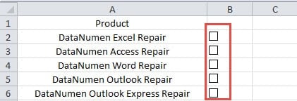

When you check one checkbox, the certain cell needs to hide or show certain contents. And below are 3 methods to achieve this task.

Method 1: Link Cells

In this method, you can link the checkboxes to certain cells.

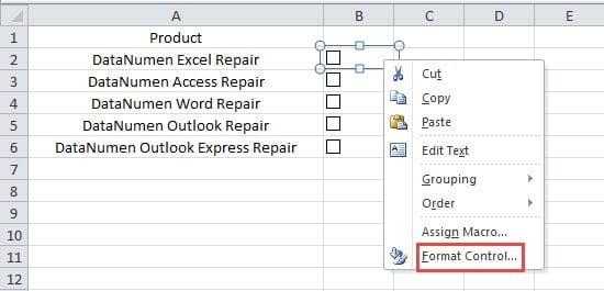
Right click one checkbox in the worksheet.
And then click the option “Format Control” in the sub menu.
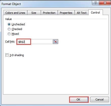
After that, input the designated cell reference into the text box of “Cell link”. Here you can also use your mouse and select the cell directly. But remember to use the absolute reference. And in this example, we use the cell B2 as the link cell.
And then click the button “OK” in the current window.

Next you will come back to the worksheet. At first, there is no content in the cell B2.

When you check the checkbox, the value “TRUE” will appear in cell B2. And then if you uncheck the checkbox, the cell will show “FALSE”.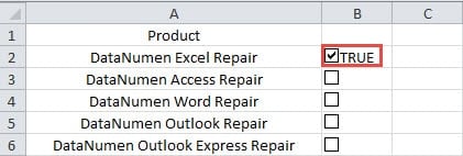

Now repeat the above steps and link other checkboxes with cells. Therefore, when the values of checkboxes change, the contents in linked cells will also change. Besides, you can also clear the contents in cells manually.

Method 2: Use IF Function

In this method, you need to make sure that the checkboxes are linked to certain cells. Thus, you can use the IF function to show certain contents.

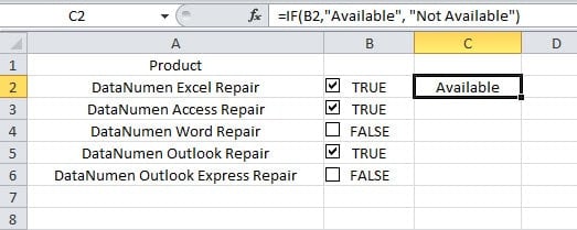
Click a cell where you need to show the contents. Here we click the cell C2 in this worksheet.
And then input the following formula into the worksheet:

=IF(B2,”Available”, “Not Available”)

Here you can see that this formula will use the result in the linked cell B2. Thus, you also need to link cells for those checkboxes. In this formula, you can also change the contents according to your need.

And then press the button “Enter” on the keyboard. Therefore, you will see the result immediately in the cell.
Now double click the fill handle of cell C2 and fill the formula in other cells.

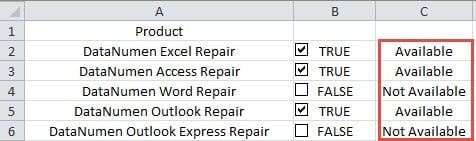
When you change the value of checkboxes, the result in cells will also change accordingly.

Method 3: Use VBA Macro

On the other hand, if you don’t want to link cells and want to show certain contents in certain cells, you can use the VBA macro. And here we will show you the steps to finish this task.

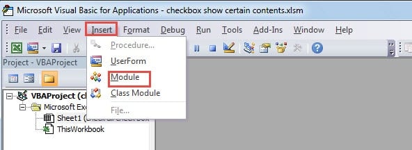
Press the shortcut keys “Alt +F11” on the keyboard.
Next click the button “Insert” in the toolbar.
And then choose the option “Module” in the drop-down menu.
Now copy the following VBA codes into the new module.

There are two procedures in the code. The first sub will show certain contents in certain cells according to the checkboxes values. And the second sub will assign the first macro to all checkboxes in batch in this worksheet. Besides, in your actual worksheet, you may also change some elements to make the VBA codes available.

And now click in the second sub.
After that, click the button “Run Sub” or press the button “F5” on the keyboard to run the second sub.
Now you can go back to the worksheet.

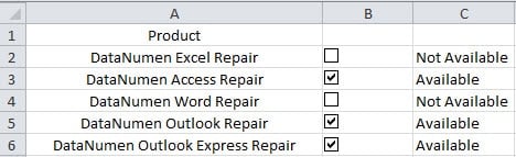
When you check or uncheck one checkbox, the contents in the certain cell will also change accordingly. And you don’t need to link cells for those checkboxes.

A Comparison between the 3 Methods

To help you choose from the 3 methods, we have listed all the possible advantages and disadvantages in the table below.

1. This method is very easy to use if you only need to show “TRUE” or “FALSE” in cells.

2. Compared with the other two methods, this is the most convenient method. 1. You can input special contents into the formula according to your need.

2. If you are not familiar with VBA macros, you can use this function to show contents. 1. All the checkboxes are assigned with macros. And you can see the contents when you check or uncheck the checkboxes.

2. You can show certain contents in cells according to your need.

1. Link cells one by one can cost you a lot of time and energy.

2. Cells can only display “TRUE” or “FALSE”, which can be inconvenient in certain situation. 1. In using this function, you also need to link cells to checkboxes one by one.

2. Showing “TRUE” or “FALSE” together with your designated contents at the same time will mess up your worksheet. 1. If you are not familiar with Excel VBA, you probably meet with problems when you run the macro.

2. Using VBA codes will make the task more complex.

From the above analysis, now you have a clear understanding about those different methods. Thus, the next time if you need to show certain contents in cells according to checkboxes values, you can choose a method according to your actual need.

Create a Backup Plan for Your Excel Files

To avoid the bad result from data disaster, one of the most effective methods is take backups for your files. Thus, whenever you meet with Excel file corruption, you will not suffer from the result. And for all your files, you need to create an effective backup plan. But condition also may exist that even the backup files are also damaged. At this moment, you can use a third party tool to repair Excel file corruption. With this recovery tool and backup files at hand, you will not loss data in a data disaster any more.

Источник

Display Cell Contents in Another Cell in Excel

Very often we reference the data of a Cell in another Cell in Excel. We can use equals to sign (=) then enter the cell address to display Cell contents in another Cell. Let us see how to display cell contents in another cell in Excel in this topic.

Referencing the Cell Contents in Another Cell

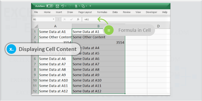
Double click on any Cell in Excel Sheet to make the Cell editable. Then enter the equals to sign (=) and enter the address of Cell which you wants to refer. You can refer a single Cell or a Range using this approach. Here are the examples on referencing the content of a Cell and displaying in another cell in Excel. Let us see the detailed examples on referencing the cells in the following scenarios.

Referencing a specific Cell
Relative Reference
Absolute Reference
Referencing a Range (multiple cells)
Referencing and Concatenating Cells
Referencing Cells from another Sheet
Referencing a Named Range
Showing Cell values on a Shape
Showing Cell value in Chart Title

It is very important to know the types of cell references we can use while referencing the cells in Excel. There are two types of references in Excel, Relative and Absolute References.

Referencing a specific Cell

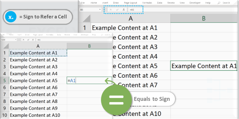
We can enter ‘=’ sign and specify the cell address in any cell in the Excel Sheet. For example, you can enter ‘=A1’ at Range B1 to refer the Cell content of A1 in B1, you can enter ‘=AB25’ at C5 to refer the content of range AB25 in Range C5.

Begin with = Sign to Refer a Cell

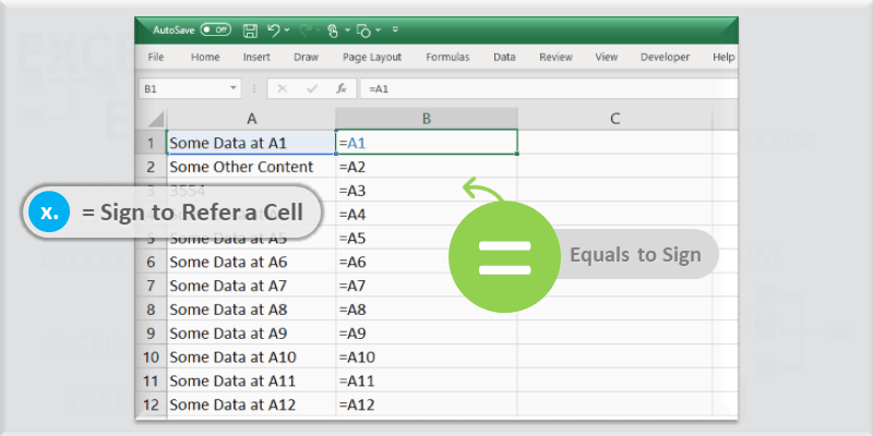
Equals to sign (=) is used to refer Cell in Another Cell

Referencing a Cell in Excel

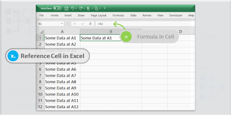
Formula Bar Showing a Cell Content in another Cell

Displaying Cell Content in Excel

Showing a Cell Content in another Cell in Excel

Fill down the Formula in Excel

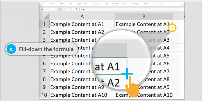
Double Click or Drag down with mouse

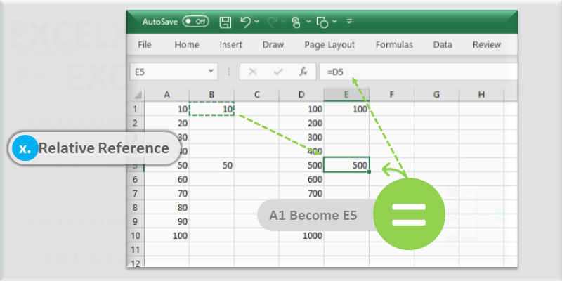
Relative Reference in Excel

Relative reference is used to change the Cell Column or Row relatively while copying the cells with formula to another range. Row number and Column Names will changes relatively when we use relative cell reference.

For example, when you have =A1 reference in Cell B1, it will change to A2 while copying down to the next row (i.e; A2), it will chnage to B1 when copying to the next Column (i.e; C1). The change in number of columns and rows depending to the relative number of columns and rows which you are pasting the cells.

For example, if you copy the same ‘=A1’ reference in Cell B1, it will change to A5 when you paste at cell B1, it will become D5 when you paste in E5.

Relative Reference in Excel

Do not use $ to create Relative Cell References

Relative Reference – Formula in Excel

Cell Formula will changes relatively in Relative Reference

Display Text From Another cell in Excel

We can display the text of another cell using Excel Formula. We can use ‘=’ assignment operator to pull the text from another cell in Excel.

For example, the following formula will get the text from Cell D5 and display in Cell B2.

You can enter =D5 in Range B2. You can use ‘$’ symbol to make the cell reference as absolute (=$D$5).

Display Value From Another cell in Excel

We can display the Value of another cell using Excel Formula. We can use ‘=’ assignment operator to pull the value of another cell in Excel.

For example, the following formula will get the value from Cell C6 and display in Cell A3.

You can enter =C6 in Range A3. You can use ‘$’ symbol to make the cell reference as absolute (=$C$6).

Referencing a Range (multiple cells)

We can refer multiple Cells in Excel using Excel Formula. We can get the cell contents and display in a cell or refer the range to perform calculations.

Getting Values From Multiple Cells in Excel

Often we refer the multiple cells in put into once Cell. We can refer the multiple Cells and Ranges in Excel to combine the text or to perform the calculations.

Getting Text from Multiple Cells

The following formula will refer the text from multiple cells and combine them to display in one Cell. This will get the contents form Cell E2 and F2 and display the combined text in another Cell.

Combine Text of Multiple Cells:

We can use & operator to concatenate the text from multiple cells. We can provide a space or – to separate the text to form multiple words. The following Example shows you how to get the data from multiple cells and display the combined text in one cell.

Getting Values from Multiple Cells:

Sometimes, we need to pull the values of another cell and perform some calculations in a cell. For example, We have Cost and Quantity values in two different cells (B2,C2) and we can find the total cost in another Cell (A2).

Combining Values of Multiple Cells:

We can also combine the numerical data of multiple cells using & operator. We can concatenate both Text and numerical data and display in required Cell. The following example shows you how to get the different formats of data from multiple cells and display the combined information in a cell.

Referring Data from a Range of Cells

The following example shows you referring a range and perform mathematical calculations. It will reference Range D1 to E5 and put the Sum of the data in Range A1

Referencing Cells from another Sheet

Referencing the Cells from one sheet is very easy in Excel. We need to pass the Sheet Name in the Formula followed by ‘!’ symbol. Exclamation symbol is used to refer the Worksheet in the Excel Formula.

The following example will refer the Cell content form another worksheet (Data) and display in a Cell.

We need to put the sheet name between single quotes when the Sheet name is having multiple words. For example the following formula will refer the Cell form another sheet named with multiple words (Data Sheet)

Referencing and Concatenating Cells

We can concatenate the Cells using Concatenate operator or using CONCATENATE Function in Excel. Let us see the both the methods to concatenate Cells in Excel.

Using Concatenate Operator: You can refer the cells using the Cell address and use the & (ampersand) operator to concatenate the Cells. For example, the following formula will concatenate cells (D1 and E1).

Using CONCATENATE Function: We can use the Excel Function to refer and concatenate multiple cells and ranges in Excel. You use the , (comma) t0 specify the reference of each Cell in the formula.

Referencing a Named Range

We can refer the Named Ranges in Excel using Formula. Name of Range should follow the = operator to refer a named range in Excel. The following Formula refer the named range called ‘TotalSales’.

The will display the Cell value which is named as ‘TotalSales’.

The following examples shows you, how to refer the range of cells in Excel. The Range (‘Sales Column’) is referred in SUM function to return the total value of ‘Sales Column’ Named Range.

Showing Cell values on a Shape

Follow the below instructions to display the cell contents on a Shape.

Select the Shape
Click on the Formula bar
Enter the = (assignment) operator
And put required Cell Address (For example: =$A$3)

Showing Cell value in Chart Title

Follow the below instructions to display the cell contents in Chart Title.

Select the Chart which you want to display the Cell Value
Go to ‘Chart Design’ Tab in the Ribbon
And Show the Chart Title from Chart Elements
Click on Chart Title of the Selected Chart
Click on the Formula bar
Enter the = (assignment) operator
And put required Cell Address (for example: =Sheet2!$K$8)

Источник

Does your Excel cell content not visible but show in formula bar? Don’t have any idea why is the text not showing in Excel cells?

Want to know how you can solve this Excel text disappears in cell mystery?

In that case, this particular post is very important to read. As it contains complete detail on how to fix Excel cell contents not visible issues.

User’s Query:

Let’s understand this issue more clearly with these user complaints.

Issue: Content of Excel cells invisible while typing

If I’m typing text or numbers into an Excel cell, while I can see what I’m writing in the formula bar above the chart, the cell shows nothing but the vertical stroke of a cursor, and no text or numbers at all until I tab out of the cell. I find this very annoying, though not a stopper to doing work. It’s unlike any Excel I’ve used in the past.

Source: https://answers.microsoft.com/en-us/msoffice/forum/all/content-of-excel-cells-invisible-while-typing/7937a331-4b27-4790-adda-9341d2010f10?auth=1

To recover lost Excel cell contents, we recommend this tool:

This software will prevent Excel workbook data such as BI data, financial reports & other analytical information from corruption and data loss. With this software you can rebuild corrupt Excel files and restore every single visual representation & dataset to its original, intact state in 3 easy steps:

Download Excel File Repair Tool rated Excellent by Softpedia, Softonic & CNET.
Select the corrupt Excel file (XLS, XLSX) & click Repair to initiate the repair process.
Preview the repaired files and click Save File to save the files at desired location.

These are the fixes that you all must try to get rid of the issue Excel cell contents not visible but show in formula bar.

1# Set The Cell Format To Text
2# Display Hidden Excel Cell Values
3# Using The Autofit Column Width Function
4# Display Cell Contents With Wrap Text Function
5# Adjust Row Height For Cell Content Visibility
6# Reposition Cell Content By Modifying The Alignment Or Rotating Text
7# Retrieve Missing Excel Cell Content

Let’s discuss all these fixes in detail….!

Fix 1# Set The Cell Format To Text

If you are facing this Excel cell contents not visible issue with a particular formula. Even after checking the formula, you haven’t found any error but still, it not showing the result.

In that case, immediately check whether the cell format is set to text or not.
You can also set the format of the cell to another suitable number format.
Now you need to get into the “cell edit mode” so that Excel can easily identify the format modification. For this just make a tap on the formula bar and hit enter.

Fix 2# Display Hidden Excel Cell Values

Choose either the range of the cell or the cells having hidden values.

Tip: you can easily cancel the cell selection, by tapping any cell present on the Excel worksheet.

Go to the Home tab and hit the Dialog Box Launcher which is present next to the Number.

Now from the Category box, tap to the General for application of the default number format.

Just tap on the number, date, or time, a format that you require.

Fix 3 # Using The Autofit Column Width Function

To display all the text not showing in Excel cell you can use the function Autofit Column Width.

It’s a very helpful feature to make easy adjustments in the column width of the cells. So this feature will, ultimately going to help in displaying all the hidden Excel cells content.

Here are the steps which you need to perform.

Choose the cell having hidden excel cell content and follow this path Home> Format > AutoFit Column Width.

After this, you will see all the cells of your worksheet will adjust their respective column width. This ultimately shows all the hidden Excel cell text.

Fix 4# Display Cell Contents With Wrap Text Function

With the Excel wrap text feature you can apply such cell formatting in which text will get wrap automatically or put a line break. After using the wrap text function your hidden excel cell content will start appearing in multiple lines.

Choose that cell whose content is not visible and tap to the Home> Wrap Text

After that, you will see your selected cell will be expanded with all the hidden content. Like this:

Note:

If still your Excel cell content not visible completely then maybe it’s because of the row size which is set to some specific height.

So follow the next solution of changing the row height to perfect content visibility.

Fix 5# Adjust Row Height For Cell Content Visibility

You can choose single or multiple rows in which you want to make a row height changes.
Go to the Home tab. Now from the Cells group choose the Format option.
Within the Cell Size, tap to the AutoFit Row Height.

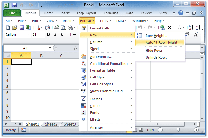
Note: for quick autofit row height of the entire worksheet cells. Just tap to the Select All button. After that make double-tap on the boundary present just below the row heading.

Fix 6# Reposition Cell Content By Modifying The Alignment Or Rotating Text

For the perfect display of data in the worksheet, you must try repositioning the text present within the cell. For this, you can make modifications in the alignment of the cell content or you can use the indentation for correct spacing. Or else display the cell content at various angles by rotating it.

1. Select the range of the cells having the data which you wish to reposition.

2. Now make a right-click over the selected rows, you will get a list of options. From which you have to choose format cells.

3. In the opened dialog box of Format Cells choose the Alignment tab and perform any of the following operations:

Change the horizontal alignment of the cell contents
Change the vertical alignment of the cell contents
Indent the cell contents
Display the cell contents vertically from top to bottom
Rotate the text in a cell
Restore the default alignment of selected cells

Fix 7# Retrieve Missing Excel Cell Content

Another very high possibility of having this Excel cell content not visible issue is worksheet corruption. As it is found that data from Excel sheet goes missing when Excel file or worksheet got corrupted.

So either you can try the manual fixes to recover corrupt Excel file data. Or else go with experts recommended solution for recovery i.e Excel repair software.

Have a look over some catchy features of this software:

This supports the entire Excel version and the demo version is free.
This is a unique tool to repair multiple Excel files at one repair cycle and recovers the entire data in a preferred location.
This is unique software to repair multiple files at once and recover everything in the preferred location.
It is easy to use and compatible with both Windows as well as Mac operating systems.
With the help of this, you can fix all sorts of issues, corruption, errors in Excel workbooks.

Wrap Up:

By trying the above-mentioned fixes you can easily fix Excel cell contents not visible but show in formula bar issue. But even if the fixes fail to display hidden Excel cell content then immediately approach the software solution.

Don’t do unnecessary delay as this will lessen the possibility of complete Excel worksheet data recovery.

Priyanka is an entrepreneur & content marketing expert. She writes tech blogs and has expertise in MS Office, Excel, and other tech subjects. Her distinctive art of presenting tech information in the easy-to-understand language is very impressive. When not writing, she loves unplanned travels.

Источник

Display Cell Contents in Another Cell in Excel

Home›Formula›Display Cell Contents in Another Cell in Excel

Display Cell Content in Another Cell in Excel

Referencing the Cell Contents in Another Cell

Referencing a specific Cell
Relative Reference
Absolute Reference
Referencing a Range (multiple cells)
Referencing and Concatenating Cells
Referencing Cells from another Sheet
Referencing a Named Range
Showing Cell values on a Shape
Showing Cell value in Chart Title

It is very important to know the types of cell references we can use while referencing the cells in Excel. There are two types of references in Excel, Relative and Absolute References.

Referencing a specific Cell

Begin with = Sign to Refer a Cell

Equals to sign (=) is used to refer Cell in Another Cell

Referencing a Cell in Excel

Formula Bar Showing a Cell Content in another Cell

Displaying Cell Content in Excel

Showing a Cell Content in another Cell in Excel

Fill down the Formula in Excel

Double Click or Drag down with mouse

Relative Reference in Excel

For example, if you copy the same ‘=A1’ reference in Cell B1, it will change to A5 when you paste at cell B1, it will become D5 when you paste in E5.

Relative Reference in Excel

Do not use $ to create Relative Cell References

Relative Reference – Formula in Excel

Cell Formula will changes relatively in Relative Reference

Display Text From Another cell in Excel

We can display the text of another cell using Excel Formula. We can use ‘=’ assignment operator to pull the text from another cell in Excel.

For example, the following formula will get the text from Cell D5 and display in Cell B2.

You can enter =D5 in Range B2. You can use ‘$’ symbol to make the cell reference as absolute (=$D$5).

Display Value From Another cell in Excel

We can display the Value of another cell using Excel Formula. We can use ‘=’ assignment operator to pull the value of another cell in Excel.

For example, the following formula will get the value from Cell C6 and display in Cell A3.

You can enter =C6 in Range A3. You can use ‘$’ symbol to make the cell reference as absolute (=$C$6).

Referencing a Range (multiple cells)

We can refer multiple Cells in Excel using Excel Formula. We can get the cell contents and display in a cell or refer the range to perform calculations.

Getting Values From Multiple Cells in Excel

Often we refer the multiple cells in put into once Cell. We can refer the multiple Cells and Ranges in Excel to combine the text or to perform the calculations.

Getting Text from Multiple Cells

The following formula will refer the text from multiple cells and combine them to display in one Cell. This will get the contents form Cell E2 and F2 and display the combined text in another Cell.

Combine Text of Multiple Cells:

Getting Values from Multiple Cells:

Combining Values of Multiple Cells:

=” Total Cost is ” &B2*C2

Referring Data from a Range of Cells

The following example shows you referring a range and perform mathematical calculations. It will reference Range D1 to E5 and put the Sum of the data in Range A1

Referencing Cells from another Sheet

The following example will refer the Cell content form another worksheet (Data) and display in a Cell.

Referencing and Concatenating Cells

We can concatenate the Cells using Concatenate operator or using CONCATENATE Function in Excel. Let us see the both the methods to concatenate Cells in Excel.

Using CONCATENATE Function: We can use the Excel Function to refer and concatenate multiple cells and ranges in Excel. You use the , (comma) t0 specify the reference of each Cell in the formula.

Referencing a Named Range

We can refer the Named Ranges in Excel using Formula. Name of Range should follow the = operator to refer a named range in Excel. The following Formula refer the named range called ‘TotalSales’.

The will display the Cell value which is named as ‘TotalSales’.

The following examples shows you, how to refer the range of cells in Excel. The Range (‘Sales Column’) is referred in SUM function to return the total value of ‘Sales Column’ Named Range.

Showing Cell values on a Shape

Follow the below instructions to display the cell contents on a Shape.

Select the Shape
Click on the Formula bar
Enter the = (assignment) operator
And put required Cell Address (For example: =$A$3)

Showing Cell value in Chart Title

Follow the below instructions to display the cell contents in Chart Title.

Select the Chart which you want to display the Cell Value
Go to ‘Chart Design’ Tab in the Ribbon
And Show the Chart Title from Chart Elements
Click on Chart Title of the Selected Chart
Click on the Formula bar
Enter the = (assignment) operator
And put required Cell Address (for example: =Sheet2!$K$8)

Share This Story, Choose Your Platform!

5 Comments

Ray
July 29, 2022 at 10:47 pm — Reply

I’d like to learn a formula that will identify a character, for example “_”, and return the contents of the next cell. The results are pulled from a data sheet and compiled into a list/column.

For example, if d:d contains “_” show contents of f:f

Any help would nmbe appreciate!
- PNRao
  September 11, 2022 at 6:51 am — Reply
```
=IF(COUNTIF(D1,"*_*"),F1,"")
```
Ian
October 5, 2022 at 4:17 am — Reply

How would you format a cell to show the content of another selected cell in the same sheet?

I’m thinking of a text search function that actively translates the content of a selected cell in a column, maybe using the Googletranslate function, but I’m currently stuck on the first part of getting the content.
Miki
February 22, 2023 at 7:20 pm — Reply

Hello!
I have a cell that contains the address of another cell. How can I get the value of this cell?
- PNRao
  February 27, 2023 at 3:13 am — Reply
  Let’s say your Cell B1 contains the address of Cell A1, and you want to get the value of Cell A1?
```
=INDIRECT(B1)
```

Page load link

Источник

In Microsoft Excel, we can easily copy the range of cells and paste it to some destination.

This can simply be done using the following steps.

Select the range of the cell
Copy the selected range using Ctrl + C command
Paste the copied cell to the destination using Ctrl + V command

But imagine a situation where we have some cells that are hidden in the range (like in the below example).

In the above data, rows 4 to 7 are hidden.

Now, if I copy this data that has hidden rows and paste it a few rows below it, something weird happens.

The hidden rows are also copied and pasted (as shown below)

By default, Excel copies the visible and hidden cells as shown in the above screenshot. So how to overcome this and only select the visible cell?

This tutorial will guide you through all the methods using which you can select the visible cell only in Excel.

Method 1: Keyboard Shortcut to Select Visible Cells Only

This is the easiest method to copy and paste the visible cell only in Excel.

Below is the keyboard shortcut to select the visible cells only:

ALT + ; (for windows)

Cmd + Shift + Z (for mac)

Let me explain it with the help of an example in which I am going to use the below dataset, where we have some Employee records with rows 4-7 hidden.

Let’s see how we can select the visible cell only. To achieve this, follow the below steps

Select the range of data that you want to copy.

Press the shortcut ALT + ; from the keyboard (hold the ALT key and then press the semicolon key). Remember the command for Mac users is Cmd + Shift + Z.

keyboard shortcut to only select visible sense

To copy the visible range, press Ctrl + C from the keyboard. Some dotted lines appear around the selection, as shown below.

Paste the cell to the destination using Ctrl + V command

copy and pasting when only visible cells are selected

This will paste only the visible cells and exclude the hidden cells, as you can see from the above screenshot.

There are other methods to perform this, which are discussed in the below sections.

Also read: How to Select Every Other Row (Alternate Row) in Excel?

Method 2: Select Visible Cells Only Using the Go to Special Dialog Box

Using the shortcut key (Alt + 😉 is a simple and easy way to copy only visible cells in Excel, but if you don’t want to remember the keyboard shortcut, you can do so by using the Go To Special option that is available in the Home tab of the ribbon.

Let me show you with the help of an example where I am going to use the same employee record data where rows 4-7 are hidden, as shown below.

Select the range of cells you want to copy.

Click on the Home tab in the ribbon

In the Home tab, click on the Find & Select option.

click the find and select option in the home tab

From the dropdown that gets open select the Go To Special option

This will open the Go To Special dialog box as shown below

Click on the option Visible cells only

select the visible cells only option in the go to special dialog box

Click on OK.

In this way, Excel will not follow the default copy-paste mechanism but only copy the visible cell.

To copy the selected range press Ctrl + C

Select the cell where you want to paste the range and press Ctrl + V

copy and pasting men only visible cells are selected

In this method, I showed you in great detail how you can use the Go To Special option to copy only visible cells.

There is another way you can do so, which is discussed in the below section.

Method 3: By Adding Select Visible Cells Option to Quick Access Toolbar

The above-discussed methods work perfectly for copying visible cells to the destination, but if you like to make it simpler, you can add the Select Visible Cells option to your Quick Access toolbar.

By doing so, you don’t have to remember the shortcut or the long process discussed in method 2.

In this method, first, I will explain how you can add a Select Visible Cells option to the toolbar, and then I will show you how you can quickly copy only visible cells using this option.

So follow all the steps to get a complete insight into the whole process.

a) Add the Select Visible Cells option to Quick Access Toolbar

Click on the Customizable Quick Access Toolbar option

click on the customizable quick access toolbar icon

From the dropdown that gets open, choose More Commands option

This will open Excel Options as shown below

Click on the ‘Choose commands from’ option

From the drop-down that gets opens, choose the “All Commands” option

select the all commands option from the drop down

This will show all the commands in Excel

Scroll down the command’s list and choose the Select Visible Cells option.

select the select visible cells only option

Click on Add

click on the add button to add the select visible sales icon to the quick access toolbar

Then click on OK

This will add the Select Visible Cells option to the toolbar as shown below

select visible sales icon is added to the quick access toolbar

b) Copy Visible Cell using the Select Visible Cells option

In the first part of this method, I showed you how you could add the Select Visible Cells option to your Quick Access Toolbar.

Now I will show you how you can employ this option to copy only visible cells just in a single click.

I am going to use the same dataset that is used in method 1 and method 2, where rows 4-7 are hidden.

Select the data that you want to copy.

Click on the Select Visible Cells icon in the Quick Access Toolbar (QAT)

click on the select visible sales icon in the quick access toolbar

Copy the data using Ctrl + C

Paste the data to the destination using Ctrl + V

copy and paste when visible cells are selected

This will only paste only the visible cell and exclude the hidden ones as shown in the above screenshot.

Tip: In the first part of this method, I also showed you how you could add the Select Visible Cells command to this Quick Access Toolbar. Similarly, you can also add any other command using the same process. Just look for the required command in the command’s list and add it using the procedure discussed in the above method.

If you’re a heavy Excel user, I am sure you will soon encounter this situation where you only need to select the visible cells (and not the hidden ones).

In this tutorial, I have discussed all the methods you can use to copy visible cells only.

I am personally a big fan of the keyboard shortcut, but in case you don’t want to burden yourself with yet another shortcut, you can add the select visible cells only icon in the Quick Access Toolbar and get this done with a single click.

Other Excel articles you may also like:

How to Select Non-adjacent Cells in Excel?
Select Row (or Rows) in Excel (Shortcut)
How to Select Rows with Specific Text in Excel
How to Select Multiple Items from a Drop Down in Excel?
How to Select Multiple Rows in Excel
How to Select Alternate Columns in Excel (or every Nth Column)
How to Select Every Other Cell in Excel (Or Every Nth Cell)
How to Paste in a Filtered Column Skipping the Hidden Cells

Источник

Sometimes, when you open an Excel spreadsheet, you can’t see the text you have typed in a cell.

The text may be visible on the formula bar but not in the cell itself. For instance, in the image below, the data in cell C2 is not visible but you can see it in the formula bar.

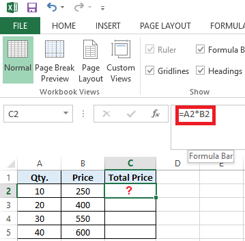
Figure 1 — Excel Not Showing Data in Cells

Also Read: Data Disappears in Excel – How to Get it Back?

Workarounds to Fix ‘Excel Not Showing Data in Cells’

Note: Before trying these workarounds, make sure that your Office program is updated.

Workaround 1 – Check for Hidden Cell Values

If cell values are hidden, you won’t be able to see data when a cell is selected. But the data will be visible in the formula bar. To display hidden cell values in a worksheet, follow these steps:

Select a single cell or range of cells that doesn’t show the text.
Right-click on the selected cell or range of cells and choose Format Cells.

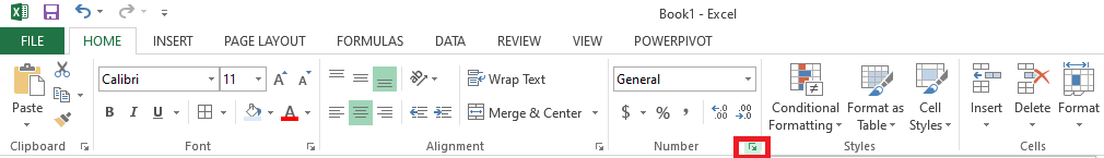
Figure 2 — Select Format Cells

A ‘Format Cells’ window opens. On the Number tab, choose Custom and check if 3 semi-colons (;;;) appear in the Type textbox.

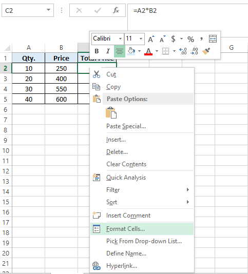
Figure 3 — Check for Semi-Colons in Type Box

If you can see the 3 semi-colons, delete them and then click OK. If you cannot see semi-colons in the ‘Type’ textbox, skip to the next workaround.

Workaround 2 – Change the Default Font

The font of cells in your Excel worksheet may be creating the problem. So, try changing the default font of cells or ranges:

Select a cell or cell range where the text is not showing up.
Right-click on the selected cell or cell range and click Format Cells.
From the pop-up window, click on the Font tab and then change the default font (usually Calibri) to any other font, like ‘Arial’ or ‘Times New Roman’. Press the OK button.

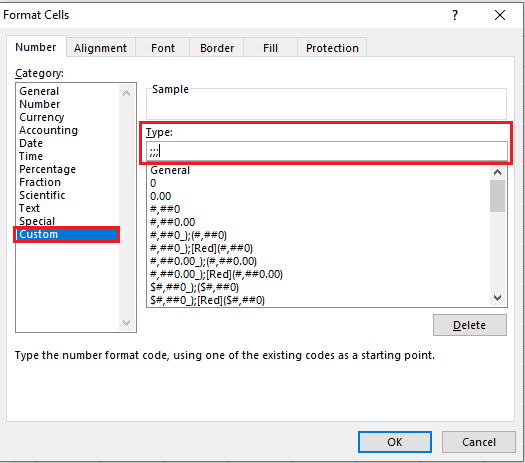
Figure 4 – Format Cells Window

If changing the default font doesn’t fix the ‘Excel data not showing in cell’ problem, proceed with the next workaround.

Workaround 3 – Disable Allow Editing Directly in Cell Option

Some users have reported that they were able to resolve the ‘Excel data not showing in cells’ issue by unchecking the ‘Allow editing directly in cells’ option. To do so, follow these steps:

In Excel, click on the File menu and then click on Options.

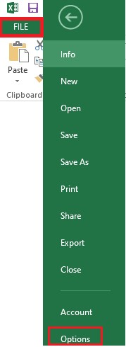
Figure 5 — Excel Options

From the Excel Options window, choose Advanced in the left pane and then uncheck ‘Allow editing directly in cells’.

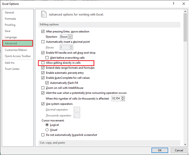
Figure 6 — Uncheck Allow Editing Directly in Cells

Click OK.

If you are unable to view the text in Excel cells, try the next workaround.

Workaround 4 – Adjust Row Height to Make the Cell Data Visible

If you have cells with wrapped text, then try adjusting the row height of the cell or range to make the data visible. Here are the steps:

Select a specific cell or range for adjusting the row height.
On the Home tab, click Format from the Cells group.

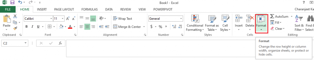
Figure 7 — Format Option in Cells Group

Under Cell Size, perform any of these actions:
Click AutoFit Row Height to automatically adjust the row height of your cell or cell range.
Click Row Height to manually enter a cell’s row height. This will open a ‘Row Height’ box. In the box, enter the row height that you want.

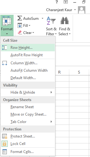
Figure 8 – Cell Size Options

Tip: You can also adjust a cell’s row height by dragging the bottom border of the row till the height when the wrapped text is visible.

Workaround 5 – Recover Missing Cell Content

Your Excel worksheet won’t display data in cells if it is corrupted. In other words, the cell values won’t display any result if the data in your Excel worksheet is damaged or corrupted. In that case, you can manually fix and recover corrupt Excel files or use an Excel repair tool, such as Stellar Repair for Excel.

Read this: How to Recover Corrupted Excel File?

Using the Excel file repair tool can help you retrieve all your worksheet data, including cell content, tables, numbers, text, rules, etc.

Wrapping Up

Oftentimes, when opening an Excel worksheet or while working on one, clicking on a cell or cell range doesn’t show any data. You may be able to see the data in the formula bar of your worksheet but not within the cells. This may prevent you from doing anything constructive in Excel. Try troubleshooting the issue by using the workarounds discussed in this article. If nothing works, chances are that corruption in the Excel file is causing it to behave oddly. Try repairing corrupt Excel file by using the built-in ‘Open and Repair’ feature or use Excel file repair software by Stellar to quickly restore your worksheet with all its data intact.

You might also be interested in reading:

[Fix] Excel formula not showing result

Easy Steps to Make Excel Hyperlinks Working

Источник