
This post will explain 7 keyboard shortcuts for the filter drop down menus. This includes my new favorite shortcut, and it’s one that I think you will really like!
This post will explain 7 keyboard shortcuts for the filter drop-down menus. This includes my new favorite shortcut, and it’s one that I think you will really like!
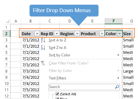
The Filter drop-down menus (formerly known as Auto Filters in Excel 2003) are an extremely useful tool for sorting and filtering your data. When the Filters are applied you will see small drop-down icon images in the header (top) row of your data range.
These menus can be accessed with keyboard shortcuts, which makes it really fast to apply filters and sorting to different columns in your table. So let’s take a look at these shortcuts.
#1 – Turn Filters On or Off
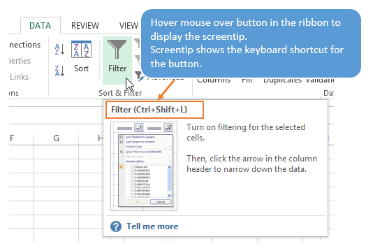
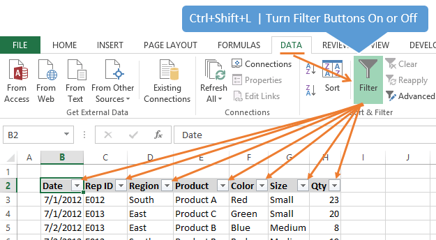
Ctrl+Shift+L is the keyboard shortcut to turn the filters on/off. You can see this shortcut by going to the Data tab on the Ribbon and hovering over the Filter button with the mouse. The screen tip will appear below the button and it displays the keyboard shortcut in the top line. This works with a lot of buttons in the ribbon and is a great way to learn keyboard shortcuts. See the image below.
To apply the drop down filters you will first need to select a cell in your data range. If your data range contains any blank columns or rows then it is best to select the entire range of cells.
Once the data cell(s) are selected, press Ctrl+Shift+L to apply the filters. The drop down filter menus should appear in the header row of your data, as shown in the image below.
#2 Display the Filter Drop Down Menu
Alt+Down Arrow is the keyboard shortcut to open the drop down menu. To use this shortcut:
- Select a cell in the header row. The cell must contain the filter drop down icon.

- Press and hold the Alt key, then press the Down Arrow key on the keyboard to open the filter menu.
Once the drop down menu is open, there are a lot of keyboard shortcuts that apply to this menu. These shortcuts are explained next.
Bonus Tip: If you are using Excel Tables, and I highly recommend you do, you can press Shift+Alt+ Down Arrow from any cell inside the table to open the filter drop-down menu for that column.
This shortcut was introduced in Excel 2010 for Windows, and works in all newer versions as well.
#3 Underlined Letters & Arrow Keys
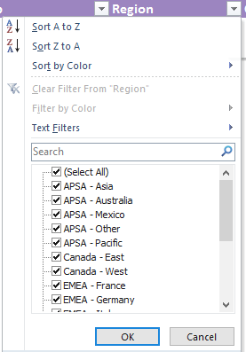
The underlined letters in the drop-down menu are the shortcut keys for each command. For example, pressing the letter “S” on the keyboard will Sort the column A to Z. You must first press Alt+Down Arrow to display the drop down menu. So here are the full keyboard shortcuts for the filter drop down menu:
- Alt+Down Arrow+S – Sort A to Z
- Alt+Down Arrow+O – Sort Z to A
- Alt+Down Arrow+T – Sort by Color sub menu
- Alt+Down Arrow+I – Filter by Color sub menu
- Alt+Down Arrow+F – Text or Date Filter sub menu

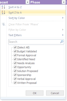
#4 Check/Uncheck Filter Items
The up and down arrow keys will move through the items in the drop down menu. You can press the Enter key to perform that action. This requires the drop down menu to be open by first pressing Alt+Down Arrow. See the image in #3 above for details.
Starting in Excel 2007, a list of unique items appears at the bottom of the filter drop down menu with check boxes next to each item. You can use the up/down arrow keys to select these items in the list. When an item is selected, pressing the space bar will check/uncheck the check box. Then press Enter to apply the filter.

#5 Search Box – My New FAVORITE
Starting in Excel 2010 a Search box was added to the filter drop-down menu. Excel 2011 for Mac users also get this feature.
This search box allows you to type a search and narrow down the results of the filter items in the list below it.

When the filter drop down menu is open, you can press the letter “E” on the keyboard to jump to the search box. This places the cursor in the search box and you can begin typing your search.
Alt+Down+Arrow+E is the shortcut to open the filter drop down menu and jump directly to the search box.
I just learned this shortcut and it is my new favorite because it makes it so fast to type and filter exactly what you are looking for in the list. Prior to learning this I was using the down arrow key to get to the search box. This required me to press the down arrow key 7 times to get to the search box. Now I can do the same thing in one step by pressing the letter “E”. What a time saver!
Bonus – Jump to the Checkbox List
If you want to jump down to the checkbox list below the Search box, you can just press Tab after Alt+Down Arrow, E.
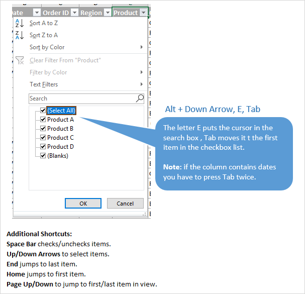
So the full keyboard shortcut is: Alt+Down Arrow, E, Tab (or Down Arrow)
You can use either the Down Arrow or Tab keys. Down Arrow will probably be easier since you just pressed Down Arrow to open the filter menu.
However, if the column contains dates then you need to press Tab twice. There is an additional drop-down menu to search by Year, Month, Date. Down Arrow opens that menu and selects each item.
Therefore, it’s probably best to get used to using Tab to get there since it works in all situations.
Once you press the shortcut, focus will be set to the (Select All) checkbox in the list box. You can then use the following shortcuts to navigate and select the checkboxes.
- Space Bar checks/unchecks items.
- Up/Down Arrows to select items.
- End jumps to last item.
- Home jumps to first item.
- Page Up/Down to jump to first/last item in view.
#6 Clear Filters in Column
Alt+Down Arrow+C will clear the filters in the selected column. Again, this is a combination of the Alt+Down Arrow to open the filter menu, then the letter “C” to clear the filter.

This would be the same as pressing the (Select All) checkbox in the item list. The next shortcut will explain how to clear all the filters in all columns.
#7 Clear All Filters
Alt+A+C is the keyboard shortcut to clear all the filters in the current filtered range. This means that all the filters in all the columns will be cleared, and all rows of your data will be displayed.
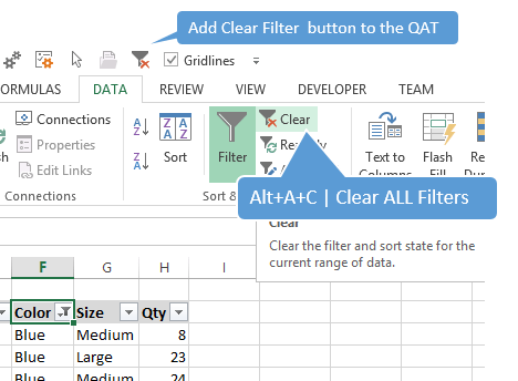
I add the Clear Filter button to the Quick Access Toolbar (QAT) and would highly recommend that you do this. It serves two purposes that are very helpful.
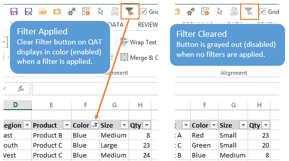
- You can quickly press the button in the QAT to clear the filters. If you are a mouse user this means you don’t have to navigate to the Data menu to access the button. You can also use keyboard shortcuts to press the buttons in the QAT. See my articles on how to setup the Quick Access Toolbar and how to use the QAT’s keyboard shortcuts for instructions on this.
_ - Use the button to visually see if any filters are applied. This is the most important benefit to me. If any filters are applied to the filter range, then the Clear Filter button in the QAT will show color (enabled). If no filters are applied then the button is grayed out (disabled). See the image below for details.
_
Debra Dalgleish has a great post and video with a few additional tips to Clear Excel Fitlers with a Single Click over at the Contextures blog.
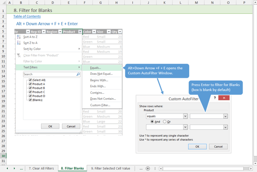
#8 Filter for Blank or Non-blank Cells or Rows
Alt+Down Arrow+F+E+Enter will filter for blanks cells in the column.
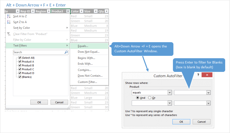
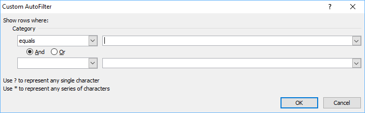
The F,E combo opens the Custom AutoFilter menu where you can type a search term. The box is blank by default. So if you just hit Enter when the Custom AutoFilter menu opens, the column will be filtered for blanks.
This is another one of my new favorites! It’s much faster than unchecking the Select All box, then scrolling to the bottom of the item list.
You can also filter for Non-blanks using the shortcut Alt+Down Arrow+F+N+Enter. This opens the Custom AutoFilter menu and sets the comparison operator to does not equal. The criteria is blank by default, so this applies a filter for non-blank cells. Thanks to Nilesh for leaving a comment and inspiring this one!
Bonus Tip
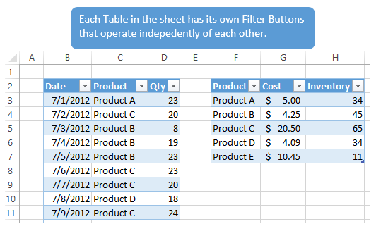
Typically you can only have one range filtered on a sheet at a time. This means that if you have more than one range of data on a sheet, you can not apply the Filters menus to both ranges.
If you use the new Excel Tables feature (introduced in Excel 2007 and available for 2011 for Mac) then you can apply Filters to each table in the same worksheet.
Checkout my video tutorial on Tables to learn more about all the great time saving benefits they have to offer.
Want More? – Download the Workbook
I hope you’ve learned some new tricks that will save you time when working with Filters. In my opinion, the keyboard shortcuts are the fastest way to work with these menus. I encourage you to practice these techniques, and also share them with a friend that might benefit.
I have also created a free workbook that contains over 25 keyboard shortcuts for the Filter Menus. The workbook is organized by topic and contains images that will help you learn the shortcuts. It also includes a data table where you can practice the shortcuts.
![]() Filter Drop-down Shortcuts Workbook.xlsx
Filter Drop-down Shortcuts Workbook.xlsx
Please click the link above and the Excel file that contains the shortcuts will be emailed to you immediately.
You will also have the option to subscribe to my free email newsletter to stay updated with new articles and videos that will help you learn Excel. After confirming your subscription you will be able to download my “10 Excel Pro Tips” eBook. It’s all free!
Challenge Question
What does the following keyboard shortcut sequence do? The selected cell must be in the header of a filtered range.
Alt+Down Arrow+E, Down Arrow, Space Bar, Shift+End, Space Bar, Enter
Please leave a comment below with your answer. Thanks!
Excel Filter Keyboard Shortcut
In Excel, sorting and filtering data is an important and common task. With the help of this, we can see the data category-wise. So, for example, if we want to see the data/record of a class subject-wise or sales data from the dozen stores that we need to keep track of, we can find the data quickly.
We can easily navigate through “Menu” or click through a mouse in less time by filtering data quickly. This article discusses keyboard excel shortcutsAn Excel shortcut is a technique of performing a manual task in a quicker way.read more used for the “Filter”.
Table of contents
- Excel Filter Keyboard Shortcut
- How to Use Keyboard Shortcut For Filter in Excel?
- Example #1 – Turn Filters ON or OFF in Excel
- Example #2 – Opening the Drop-down Filter Menu in Excel
- Example #3 – Select Menu Items Using Arrow keys
- Example #4 – Drop Down Menu Keyboard Shortcut for Filter in Excel
- Example #5 – Clear All Filters in the Current Filtered Range in Excel
- Example #6 – Clear Filter in a Column
- Example #7 – Display the Custom Filter Dialog Box
- Things to Remember About Filter Shortcut in Excel
- Recommended Articles
- How to Use Keyboard Shortcut For Filter in Excel?
How to Use Keyboard Shortcut For Filter in Excel?
Let us understand the “Filter” shortcut in Excel with examples below.
You can download this Filter Shortcut Excel Template here – Filter Shortcut Excel Template
Example #1 – Turn Filters ON or OFF in Excel
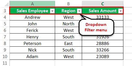
We have given below sales data region-wise.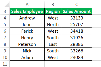
For this, follow the below steps:
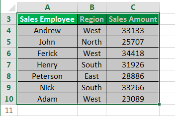
- First, we must select a cell in the data range. Then, if the data range contains any blank columns or rows, choose the entire range of cells.

- Next, we must go to the “Data” tab. Then, click on the “Filter” option under the “Sort & Filter” section. You may refer to the below screenshot.

We can also use the keyboard shortcut “CTRL+SHIFT+L” to turn on/off the filters.

- On applying the filter, the drop-down filter menus may appear in the header row of the data. For example, refer to the below screenshot.


Once the filter has been enabled on the data, we can use the drop-down menus on each column header. Follow the below steps for doing the same:
- We must first select a cell in the header row. As we can see, every cell contains a drop-down icon like the image. Then, press the “ALT + down arrow key” on the keyboard to open the “Filter” menu like the below screenshot.
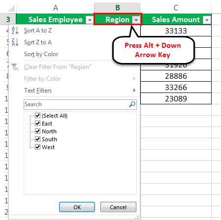
- We can see in the above image that there are many keyboard shortcuts available in the “Text Filters” menu.
Once the excel filter is enabled, we can use arrow keys to navigate the “Filter” menu. First, we must use the “Enter” and “Spacebar” keys to select and apply to the filter. Remember the below points:
- We must press the “Up and Down arrow” keys to select a command.
- Next, we must press the “Enter” key to apply the command.
- Finally, we must press the “Spacebar” key to check and uncheck the checkbox.
It would help if we first press the “ALT+ Down arrow” key to display the drop-down menu. With this, we can use any one of the following:
- S – Sort A to Z
- O – Sort Z to A
- T – Sort by ColorWhen a column or a data range in excel is formatted with colors either by using the conditional formatting or manually, when we use filter on the data excel provides us with an option to sort the data by color, there is also an option for advanced sort where user can enter different levels of color for sorting.read more submenu
- C – Clear filter
- I – Filter by Color submenu
- F – Text Filters
- E-Text Box
Example #5 – Clear All Filters in the Current Filtered Range in Excel
We can press the “ALT+Down Arrow+C” shortcut key to clear all the filters in the current filtered range. Moreover, it may remove all the filters in all the columns. After that, it will display all rows of the data.

For this, we also can use the Excel ribbonThe ribbon is an element of the UI (User Interface) which is seen as a strip that consists of buttons or tabs; it is available at the top of the excel sheet. This option was first introduced in the Microsoft Excel 2007.read more option.
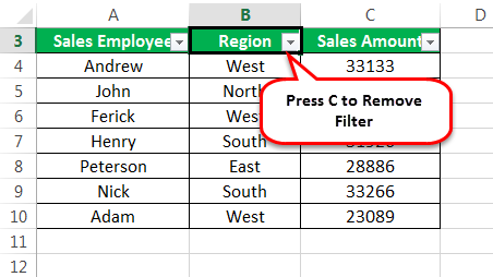
Example #6 – Clear Filter in a Column
To clear filter in a column, follow the below steps:
- First, select a cell in the header row and press “Alt+Down Arrow” to display the “Filter” menu for the column.

- Then, press the letter “C” to clear the filter.
Example #7 – Display the Custom AutoFilter Dialog Box
We can use a “Custom AutoFilter” dialog box when we want to filter the data by using the custom criteria. For this, we can follow the below steps:
- First, we must select a cell in the header row.
- Then, press the “ALT+Down Arrow” key to display the “Filter” menu for the column.
- Next, type the letter “F.”
- Finally, type the letter” E.”
- As a result, a “Custom AutoFilter” dialog box may appear, setting the comparison operator to equal. See the below screenshot.

- After that, select the option from the list (such as not equal, etc.) and insert the criteria.
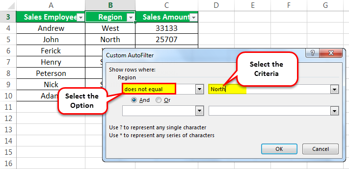
- Select “And” or “Or,” then press “OK” to apply the filter.

Consequently, it may display the filtered data.

Things to Remember About Filter Shortcut in Excel
- Using the Excel tables featureIn excel, tables are a range with data in rows and columns, and they expand when new data is inserted in the range in any new row or column in the table. To use a table, click on the table and select the data range.read more, we can apply the filters on more than one table range in the same worksheet.
- Using the filters keyboard shortcut in Excel, we can save a lot of time.
- This article explains that keyboard shortcuts are the fastest to work with filter menus.
Recommended Articles
This article is a guide to Filter Shortcut in Excel. Here, we discuss how to use keyboard shortcuts for a filter in Excel in different ways, practical examples, and downloadable Excel templates. You may learn more about Excel from the following articles: –
- How to Add and Use Filter in Excel?
- Advanced Filter in Excel
- Auto Filter In Excel
- AutoFill in Excel
Reader Interactions
How to Filter Microsoft Excel Data Quickly using Keyboard Shortcuts
by Avantix Learning Team | Updated October 20, 2021
Applies to: Microsoft® Excel® 2010, 2013, 2016, 2019 and 365 (Windows)
You can turn on filtering (formerly known as auto filtering) for Microsoft Excel lists and tables and easily filter and sort data using a mouse. When you first turn on filtering, arrows appear in the header row for each field with a drop-down menu.
Although most users will use the mouse to apply and remove filtering, you can also use your keyboard. The shortcuts are available in Excel 2010 and later versions but some will also work in 2007.
Recommended article: How to Enter Data in an Excel Filtered List into Visible Cells (2 Ways)
Do you want to learn more about Excel? Check out our virtual classroom or live classroom Excel courses >
The following are 10 useful keyboard shortcuts for filtering.
1. Turning filtering on or off
To turn filtering on or off, ensure a cell in the range is selected and then press Ctrl + Shift + L.
Down arrows will appear beside field names in the header row as follows:
![]()
If your data range contains any blank columns or rows, select the entire range of cells first.
If you have converted a list to a table, the Filter menus should automatically appear.
2. Displaying the Filter menu
To display the Filter menu for a column:
- Select a cell in the header row that contains a Filter arrow.
- Press Alt + down arrow to display the Filter menu for the column.
If your data has been converted to a table, you can press Alt + Shift + down arrow in any cell in the table to display the Filter menu for that column.
3. Selecting menu items using arrow keys
Once the Filter menu is displayed, you can use your arrow keys to navigate the menu and use Enter and the Spacebar to select and apply filtering:
- Press the up or down arrow keys to select a command.
- Press Enter to apply the command.
- Press the Spacebar to check or uncheck a checkbox.
4. Clearing all filters
To clear all filters for all fields in the current filtered range, select a cell in the range and press Alt > A > C.
Don’t press Shift and don’t press these keys at the same time as they access the Ribbon. Simply press Alt, then A, then C.
You can also press Ctrl + Shift + L t turn filtering off which will remove the filters. Press Ctrl + Shift + L to turn filtering on again.
5. Clearing filters in a column
To clear the filters in a column:
- Select a cell in the header row and press Alt + down arrow to display the Filter menu for the column.
- Type the letter «C» to clear the filter.
6. Filtering by typing underlined characters
Once the Filter menu is displayed, you can type underlined letters to select a filter option. The underlined letters that appear in the menu are the shortcut keys for each command. For example, typing the letter «F» would display the Text, Number or Date Filters sub-menu. Don’t press Shift while typing these characters.
Note the underlined characters in the menu below:
7. Sorting by typing underlined characters
Once the Filter menu is displayed, you can type characters to sort (do not hold down Shift):
- Type «S» to sort in ascending order.
- Type «O» to sort in descending order.
- Type «T» to sort by color.
8. Filtering using the Search box
Starting in Excel 2010, a Search box was added to the Filter menu. You can enter search criteria in the Search box and Excel will automatically filter in the column.
To use the Search box:
- Select a cell in the header row and press Alt + down arrow to display the Filter menu for the selected column.
- Type the letter «E» to jump to the Search box where you can type your criteria.
Note the Search box in the menu below:
9. Displaying the Custom Filter dialog box
When you want to filter using custom criteria, you can display the Custom Filter dialog box:
- Select a cell in the header row and press Alt + down arrow to display the Filter menu for the column.
- Type the letter «F».
- Type the letter «E» (this displays the Custom Filter dialog box which sets the comparison operator to Equal).
- Select options from the menus (such as Equal, Not Equal, etc.) and enter criteria.
- Select And or Or.
- Press Enter to apply the filter.
Enter criteria in criteria boxes in the Custom Filter (AutoFilter) dialog box below:
In the Custom Filter dialog box, you can keep pressing Tab to select different options in the dialog.
10. Filtering blanks or non-blanks
To filter to display blank cells in the selected column:
- Press Alt + down arrow to display the Filter menu for the column.
- Type the letter «F».
- Type the letter «E» (this displays the Custom Filter dialog box which sets the comparison operator to Equal).
- Press Enter.
To filter to display non-blank cells in the selected column:
- Press Alt + down arrow to display the Filter menu for the column.
- Type the letter «F».
- Type the letter «N» (this displays the Custom Filter dialog box which sets the comparison operator to Does Not Equal).
- Press Enter.
If you use filtering a lot, these keyboard shortcuts can save you quite a bit of time.
Subscribe to get more articles like this one
Did you find this article helpful? If you would like to receive new articles, JOIN our email list.
More resources
How to Convert Seconds to Minutes and Seconds in Excel
3 Excel Strikethrough Shortcuts to Cross Out Text or Values in Cells
How to Delete Blank Rows in Excel (5 Fast Ways to Remove Empty Rows)
How to Change Commas to Decimal Points in Excel and Vice Versa (5 Ways)
How to Replace Blank Cells in Excel with Zeros (0), Dashes (-) or Other Values
Related courses
Microsoft Excel: Intermediate / Advanced
Microsoft Excel: Data Analysis with Functions, Dashboards and What-If Analysis Tools
Microsoft Excel: Introduction to Visual Basic for Applications (VBA)
VIEW MORE COURSES >
Our instructor-led courses are delivered in virtual classroom format or at our downtown Toronto location at 18 King Street East, Suite 1400, Toronto, Ontario, Canada (some in-person classroom courses may also be delivered at an alternate downtown Toronto location). Contact us at info@avantixlearning.ca if you’d like to arrange custom instructor-led virtual classroom or onsite training on a date that’s convenient for you.
Copyright 2023 Avantix® Learning
Microsoft, the Microsoft logo, Microsoft Office and related Microsoft applications and logos are registered trademarks of Microsoft Corporation in Canada, US and other countries. All other trademarks are the property of the registered owners.
Avantix Learning |18 King Street East, Suite 1400, Toronto, Ontario, Canada M5C 1C4 | Contact us at info@avantixlearning.ca
Many users find that using an external keyboard with keyboard shortcuts for Excel helps them work more efficiently. For users with mobility or vision disabilities, keyboard shortcuts can be easier than using the touchscreen and are an essential alternative to using a mouse.
Notes:
-
The shortcuts in this topic refer to the US keyboard layout. Keys for other layouts might not correspond exactly to the keys on a US keyboard.
-
A plus sign (+) in a shortcut means that you need to press multiple keys at the same time.
-
A comma sign (,) in a shortcut means that you need to press multiple keys in order.
This article describes the keyboard shortcuts, function keys, and some other common shortcut keys in Excel for Windows.
Notes:
-
To quickly find a shortcut in this article, you can use the Search. Press Ctrl+F, and then type your search words.
-
If an action that you use often does not have a shortcut key, you can record a macro to create one. For instructions, go to Automate tasks with the Macro Recorder.
-
Download our 50 time-saving Excel shortcuts quick tips guide.
-
Get the Excel 2016 keyboard shortcuts in a Word document: Excel keyboard shortcuts and function keys.
In this topic
-
Frequently used shortcuts
-
Ribbon keyboard shortcuts
-
Use the Access keys for ribbon tabs
-
Work in the ribbon with the keyboard
-
-
Keyboard shortcuts for navigating in cells
-
Keyboard shortcuts for formatting cells
-
Keyboard shortcuts in the Paste Special dialog box in Excel 2013
-
-
Keyboard shortcuts for making selections and performing actions
-
Keyboard shortcuts for working with data, functions, and the formula bar
-
Keyboard shortcuts for refreshing external data
-
Power Pivot keyboard shortcuts
-
Function keys
-
Other useful shortcut keys
Frequently used shortcuts
This table lists the most frequently used shortcuts in Excel.
|
To do this |
Press |
|---|---|
|
Close a workbook. |
Ctrl+W |
|
Open a workbook. |
Ctrl+O |
|
Go to the Home tab. |
Alt+H |
|
Save a workbook. |
Ctrl+S |
|
Copy selection. |
Ctrl+C |
|
Paste selection. |
Ctrl+V |
|
Undo recent action. |
Ctrl+Z |
|
Remove cell contents. |
Delete |
|
Choose a fill color. |
Alt+H, H |
|
Cut selection. |
Ctrl+X |
|
Go to the Insert tab. |
Alt+N |
|
Apply bold formatting. |
Ctrl+B |
|
Center align cell contents. |
Alt+H, A, C |
|
Go to the Page Layout tab. |
Alt+P |
|
Go to the Data tab. |
Alt+A |
|
Go to the View tab. |
Alt+W |
|
Open the context menu. |
Shift+F10 or Windows Menu key |
|
Add borders. |
Alt+H, B |
|
Delete column. |
Alt+H, D, C |
|
Go to the Formula tab. |
Alt+M |
|
Hide the selected rows. |
Ctrl+9 |
|
Hide the selected columns. |
Ctrl+0 |
Top of Page
Ribbon keyboard shortcuts
The ribbon groups related options on tabs. For example, on the Home tab, the Number group includes the Number Format option. Press the Alt key to display the ribbon shortcuts, called Key Tips, as letters in small images next to the tabs and options as shown in the image below.
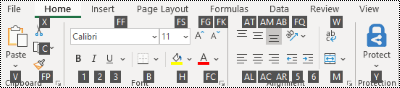
You can combine the Key Tips letters with the Alt key to make shortcuts called Access Keys for the ribbon options. For example, press Alt+H to open the Home tab, and Alt+Q to move to the Tell me or Search field. Press Alt again to see KeyTips for the options for the selected tab.
Depending on the version of Microsoft 365 you are using, the Search text field at the top of the app window might be called Tell Me instead. Both offer a largely similar experience, but some options and search results can vary.
In Office 2013 and Office 2010, most of the old Alt key menu shortcuts still work, too. However, you need to know the full shortcut. For example, press Alt, and then press one of the old menu keys, for example, E (Edit), V (View), I (Insert), and so on. A notification pops up saying you’re using an access key from an earlier version of Microsoft 365. If you know the entire key sequence, go ahead, and use it. If you don’t know the sequence, press Esc and use Key Tips instead.
Use the Access keys for ribbon tabs
To go directly to a tab on the ribbon, press one of the following access keys. Additional tabs might appear depending on your selection in the worksheet.
|
To do this |
Press |
|---|---|
|
Move to the Tell me or Search field on the ribbon and type a search term for assistance or Help content. |
Alt+Q, then enter the search term. |
|
Open the File menu. |
Alt+F |
|
Open the Home tab and format text and numbers and use the Find tool. |
Alt+H |
|
Open the Insert tab and insert PivotTables, charts, add-ins, Sparklines, pictures, shapes, headers, or text boxes. |
Alt+N |
|
Open the Page Layout tab and work with themes, page setup, scale, and alignment. |
Alt+P |
|
Open the Formulas tab and insert, trace, and customize functions and calculations. |
Alt+M |
|
Open the Data tab and connect to, sort, filter, analyze, and work with data. |
Alt+A |
|
Open the Review tab and check spelling, add notes and threaded comments, and protect sheets and workbooks. |
Alt+R |
|
Open the View tab and preview page breaks and layouts, show and hide gridlines and headings, set zoom magnification, manage windows and panes, and view macros. |
Alt+W |
Top of Page
Work in the ribbon with the keyboard
|
To do this |
Press |
|---|---|
|
Select the active tab on the ribbon and activate the access keys. |
Alt or F10. To move to a different tab, use access keys or the arrow keys. |
|
Move the focus to commands on the ribbon. |
Tab key or Shift+Tab |
|
Move down, up, left, or right, respectively, among the items on the ribbon. |
Arrow keys |
|
Show the tooltip for the ribbon element currently in focus. |
Ctrl+Shift+F10 |
|
Activate a selected button. |
Spacebar or Enter |
|
Open the list for a selected command. |
Down arrow key |
|
Open the menu for a selected button. |
Alt+Down arrow key |
|
When a menu or submenu is open, move to the next command. |
Down arrow key |
|
Expand or collapse the ribbon. |
Ctrl+F1 |
|
Open a context menu. |
Shift+F10 Or, on a Windows keyboard, the Windows Menu key (usually between the Alt Gr and right Ctrl keys) |
|
Move to the submenu when a main menu is open or selected. |
Left arrow key |
|
Move from one group of controls to another. |
Ctrl+Left or Right arrow key |
Top of Page
Keyboard shortcuts for navigating in cells
|
To do this |
Press |
|---|---|
|
Move to the previous cell in a worksheet or the previous option in a dialog box. |
Shift+Tab |
|
Move one cell up in a worksheet. |
Up arrow key |
|
Move one cell down in a worksheet. |
Down arrow key |
|
Move one cell left in a worksheet. |
Left arrow key |
|
Move one cell right in a worksheet. |
Right arrow key |
|
Move to the edge of the current data region in a worksheet. |
Ctrl+Arrow key |
|
Enter the End mode, move to the next nonblank cell in the same column or row as the active cell, and turn off End mode. If the cells are blank, move to the last cell in the row or column. |
End, Arrow key |
|
Move to the last cell on a worksheet, to the lowest used row of the rightmost used column. |
Ctrl+End |
|
Extend the selection of cells to the last used cell on the worksheet (lower-right corner). |
Ctrl+Shift+End |
|
Move to the cell in the upper-left corner of the window when Scroll lock is turned on. |
Home+Scroll lock |
|
Move to the beginning of a worksheet. |
Ctrl+Home |
|
Move one screen down in a worksheet. |
Page down |
|
Move to the next sheet in a workbook. |
Ctrl+Page down |
|
Move one screen to the right in a worksheet. |
Alt+Page down |
|
Move one screen up in a worksheet. |
Page up |
|
Move one screen to the left in a worksheet. |
Alt+Page up |
|
Move to the previous sheet in a workbook. |
Ctrl+Page up |
|
Move one cell to the right in a worksheet. Or, in a protected worksheet, move between unlocked cells. |
Tab key |
|
Open the list of validation choices on a cell that has data validation option applied to it. |
Alt+Down arrow key |
|
Cycle through floating shapes, such as text boxes or images. |
Ctrl+Alt+5, then the Tab key repeatedly |
|
Exit the floating shape navigation and return to the normal navigation. |
Esc |
|
Scroll horizontally. |
Ctrl+Shift, then scroll your mouse wheel up to go left, down to go right |
|
Zoom in. |
Ctrl+Alt+Equal sign ( = ) |
|
Zoom out. |
Ctrl+Alt+Minus sign (-) |
Top of Page
Keyboard shortcuts for formatting cells
|
To do this |
Press |
|---|---|
|
Open the Format Cells dialog box. |
Ctrl+1 |
|
Format fonts in the Format Cells dialog box. |
Ctrl+Shift+F or Ctrl+Shift+P |
|
Edit the active cell and put the insertion point at the end of its contents. Or, if editing is turned off for the cell, move the insertion point into the formula bar. If editing a formula, toggle Point mode off or on so you can use the arrow keys to create a reference. |
F2 |
|
Insert a note. Open and edit a cell note. |
Shift+F2 Shift+F2 |
|
Insert a threaded comment. Open and reply to a threaded comment. |
Ctrl+Shift+F2 Ctrl+Shift+F2 |
|
Open the Insert dialog box to insert blank cells. |
Ctrl+Shift+Plus sign (+) |
|
Open the Delete dialog box to delete selected cells. |
Ctrl+Minus sign (-) |
|
Enter the current time. |
Ctrl+Shift+Colon (:) |
|
Enter the current date. |
Ctrl+Semicolon (;) |
|
Switch between displaying cell values or formulas in the worksheet. |
Ctrl+Grave accent (`) |
|
Copy a formula from the cell above the active cell into the cell or the formula bar. |
Ctrl+Apostrophe (‘) |
|
Move the selected cells. |
Ctrl+X |
|
Copy the selected cells. |
Ctrl+C |
|
Paste content at the insertion point, replacing any selection. |
Ctrl+V |
|
Open the Paste Special dialog box. |
Ctrl+Alt+V |
|
Italicize text or remove italic formatting. |
Ctrl+I or Ctrl+3 |
|
Bold text or remove bold formatting. |
Ctrl+B or Ctrl+2 |
|
Underline text or remove underline. |
Ctrl+U or Ctrl+4 |
|
Apply or remove strikethrough formatting. |
Ctrl+5 |
|
Switch between hiding objects, displaying objects, and displaying placeholders for objects. |
Ctrl+6 |
|
Apply an outline border to the selected cells. |
Ctrl+Shift+Ampersand sign (&) |
|
Remove the outline border from the selected cells. |
Ctrl+Shift+Underscore (_) |
|
Display or hide the outline symbols. |
Ctrl+8 |
|
Use the Fill Down command to copy the contents and format of the topmost cell of a selected range into the cells below. |
Ctrl+D |
|
Apply the General number format. |
Ctrl+Shift+Tilde sign (~) |
|
Apply the Currency format with two decimal places (negative numbers in parentheses). |
Ctrl+Shift+Dollar sign ($) |
|
Apply the Percentage format with no decimal places. |
Ctrl+Shift+Percent sign (%) |
|
Apply the Scientific number format with two decimal places. |
Ctrl+Shift+Caret sign (^) |
|
Apply the Date format with the day, month, and year. |
Ctrl+Shift+Number sign (#) |
|
Apply the Time format with the hour and minute, and AM or PM. |
Ctrl+Shift+At sign (@) |
|
Apply the Number format with two decimal places, thousands separator, and minus sign (-) for negative values. |
Ctrl+Shift+Exclamation point (!) |
|
Open the Insert hyperlink dialog box. |
Ctrl+K |
|
Check spelling in the active worksheet or selected range. |
F7 |
|
Display the Quick Analysis options for selected cells that contain data. |
Ctrl+Q |
|
Display the Create Table dialog box. |
Ctrl+L or Ctrl+T |
|
Open the Workbook Statistics dialog box. |
Ctrl+Shift+G |
Top of Page
Keyboard shortcuts in the Paste Special dialog box in Excel 2013
In Excel 2013, you can paste a specific aspect of the copied data like its formatting or value using the Paste Special options. After you’ve copied the data, press Ctrl+Alt+V, or Alt+E+S to open the Paste Special dialog box.
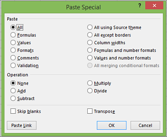
Tip: You can also select Home > Paste > Paste Special.
To pick an option in the dialog box, press the underlined letter for that option. For example, press the letter C to pick the Comments option.
|
To do this |
Press |
|---|---|
|
Paste all cell contents and formatting. |
A |
|
Paste only the formulas as entered in the formula bar. |
F |
|
Paste only the values (not the formulas). |
V |
|
Paste only the copied formatting. |
T |
|
Paste only comments and notes attached to the cell. |
C |
|
Paste only the data validation settings from copied cells. |
N |
|
Paste all cell contents and formatting from copied cells. |
H |
|
Paste all cell contents without borders. |
X |
|
Paste only column widths from copied cells. |
W |
|
Paste only formulas and number formats from copied cells. |
R |
|
Paste only the values (not formulas) and number formats from copied cells. |
U |
Top of Page
Keyboard shortcuts for making selections and performing actions
|
To do this |
Press |
|---|---|
|
Select the entire worksheet. |
Ctrl+A or Ctrl+Shift+Spacebar |
|
Select the current and next sheet in a workbook. |
Ctrl+Shift+Page down |
|
Select the current and previous sheet in a workbook. |
Ctrl+Shift+Page up |
|
Extend the selection of cells by one cell. |
Shift+Arrow key |
|
Extend the selection of cells to the last nonblank cell in the same column or row as the active cell, or if the next cell is blank, to the next nonblank cell. |
Ctrl+Shift+Arrow key |
|
Turn extend mode on and use the arrow keys to extend a selection. Press again to turn off. |
F8 |
|
Add a non-adjacent cell or range to a selection of cells by using the arrow keys. |
Shift+F8 |
|
Start a new line in the same cell. |
Alt+Enter |
|
Fill the selected cell range with the current entry. |
Ctrl+Enter |
|
Complete a cell entry and select the cell above. |
Shift+Enter |
|
Select an entire column in a worksheet. |
Ctrl+Spacebar |
|
Select an entire row in a worksheet. |
Shift+Spacebar |
|
Select all objects on a worksheet when an object is selected. |
Ctrl+Shift+Spacebar |
|
Extend the selection of cells to the beginning of the worksheet. |
Ctrl+Shift+Home |
|
Select the current region if the worksheet contains data. Press a second time to select the current region and its summary rows. Press a third time to select the entire worksheet. |
Ctrl+A or Ctrl+Shift+Spacebar |
|
Select the current region around the active cell. |
Ctrl+Shift+Asterisk sign (*) |
|
Select the first command on the menu when a menu or submenu is visible. |
Home |
|
Repeat the last command or action, if possible. |
Ctrl+Y |
|
Undo the last action. |
Ctrl+Z |
|
Expand grouped rows or columns. |
While hovering over the collapsed items, press and hold the Shift key and scroll down. |
|
Collapse grouped rows or columns. |
While hovering over the expanded items, press and hold the Shift key and scroll up. |
Top of Page
Keyboard shortcuts for working with data, functions, and the formula bar
|
To do this |
Press |
|---|---|
|
Turn on or off tooltips for checking formulas directly in the formula bar or in the cell you’re editing. |
Ctrl+Alt+P |
|
Edit the active cell and put the insertion point at the end of its contents. Or, if editing is turned off for the cell, move the insertion point into the formula bar. If editing a formula, toggle Point mode off or on so you can use the arrow keys to create a reference. |
F2 |
|
Expand or collapse the formula bar. |
Ctrl+Shift+U |
|
Cancel an entry in the cell or formula bar. |
Esc |
|
Complete an entry in the formula bar and select the cell below. |
Enter |
|
Move the cursor to the end of the text when in the formula bar. |
Ctrl+End |
|
Select all text in the formula bar from the cursor position to the end. |
Ctrl+Shift+End |
|
Calculate all worksheets in all open workbooks. |
F9 |
|
Calculate the active worksheet. |
Shift+F9 |
|
Calculate all worksheets in all open workbooks, regardless of whether they have changed since the last calculation. |
Ctrl+Alt+F9 |
|
Check dependent formulas, and then calculate all cells in all open workbooks, including cells not marked as needing to be calculated. |
Ctrl+Alt+Shift+F9 |
|
Display the menu or message for an Error Checking button. |
Alt+Shift+F10 |
|
Display the Function Arguments dialog box when the insertion point is to the right of a function name in a formula. |
Ctrl+A |
|
Insert argument names and parentheses when the insertion point is to the right of a function name in a formula. |
Ctrl+Shift+A |
|
Insert the AutoSum formula |
Alt+Equal sign ( = ) |
|
Invoke Flash Fill to automatically recognize patterns in adjacent columns and fill the current column |
Ctrl+E |
|
Cycle through all combinations of absolute and relative references in a formula if a cell reference or range is selected. |
F4 |
|
Insert a function. |
Shift+F3 |
|
Copy the value from the cell above the active cell into the cell or the formula bar. |
Ctrl+Shift+Straight quotation mark («) |
|
Create an embedded chart of the data in the current range. |
Alt+F1 |
|
Create a chart of the data in the current range in a separate Chart sheet. |
F11 |
|
Define a name to use in references. |
Alt+M, M, D |
|
Paste a name from the Paste Name dialog box (if names have been defined in the workbook). |
F3 |
|
Move to the first field in the next record of a data form. |
Enter |
|
Create, run, edit, or delete a macro. |
Alt+F8 |
|
Open the Microsoft Visual Basic For Applications Editor. |
Alt+F11 |
|
Open the Power Query Editor |
Alt+F12 |
Top of Page
Keyboard shortcuts for refreshing external data
Use the following keys to refresh data from external data sources.
|
To do this |
Press |
|---|---|
|
Stop a refresh operation. |
Esc |
|
Refresh data in the current worksheet. |
Ctrl+F5 |
|
Refresh all data in the workbook. |
Ctrl+Alt+F5 |
Top of Page
Power Pivot keyboard shortcuts
Use the following keyboard shortcuts with Power Pivot in Microsoft 365, Excel 2019, Excel 2016, and Excel 2013.
|
To do this |
Press |
|---|---|
|
Open the context menu for the selected cell, column, or row. |
Shift+F10 |
|
Select the entire table. |
Ctrl+A |
|
Copy selected data. |
Ctrl+C |
|
Delete the table. |
Ctrl+D |
|
Move the table. |
Ctrl+M |
|
Rename the table. |
Ctrl+R |
|
Save the file. |
Ctrl+S |
|
Redo the last action. |
Ctrl+Y |
|
Undo the last action. |
Ctrl+Z |
|
Select the current column. |
Ctrl+Spacebar |
|
Select the current row. |
Shift+Spacebar |
|
Select all cells from the current location to the last cell of the column. |
Shift+Page down |
|
Select all cells from the current location to the first cell of the column. |
Shift+Page up |
|
Select all cells from the current location to the last cell of the row. |
Shift+End |
|
Select all cells from the current location to the first cell of the row. |
Shift+Home |
|
Move to the previous table. |
Ctrl+Page up |
|
Move to the next table. |
Ctrl+Page down |
|
Move to the first cell in the upper-left corner of selected table. |
Ctrl+Home |
|
Move to the last cell in the lower-right corner of selected table. |
Ctrl+End |
|
Move to the first cell of the selected row. |
Ctrl+Left arrow key |
|
Move to the last cell of the selected row. |
Ctrl+Right arrow key |
|
Move to the first cell of the selected column. |
Ctrl+Up arrow key |
|
Move to the last cell of selected column. |
Ctrl+Down arrow key |
|
Close a dialog box or cancel a process, such as a paste operation. |
Ctrl+Esc |
|
Open the AutoFilter Menu dialog box. |
Alt+Down arrow key |
|
Open the Go To dialog box. |
F5 |
|
Recalculate all formulas in the Power Pivot window. For more information, see Recalculate Formulas in Power Pivot. |
F9 |
Top of Page
Function keys
|
Key |
Description |
|---|---|
|
F1 |
|
|
F2 |
|
|
F3 |
|
|
F4 |
|
|
F5 |
|
|
F6 |
|
|
F7 |
|
|
F8 |
|
|
F9 |
|
|
F10 |
|
|
F11 |
|
|
F12 |
|
Top of Page
Other useful shortcut keys
|
Key |
Description |
|---|---|
|
Alt |
For example,
|
|
Arrow keys |
|
|
Backspace |
|
|
Delete |
|
|
End |
|
|
Enter |
|
|
Esc |
|
|
Home |
|
|
Page down |
|
|
Page up |
|
|
Shift |
|
|
Spacebar |
|
|
Tab key |
|
Top of Page
See also
Excel help & learning
Basic tasks using a screen reader with Excel
Use a screen reader to explore and navigate Excel
Screen reader support for Excel
This article describes the keyboard shortcuts, function keys, and some other common shortcut keys in Excel for Mac.
Notes:
-
The settings in some versions of the Mac operating system (OS) and some utility applications might conflict with keyboard shortcuts and function key operations in Microsoft 365 for Mac.
-
If you don’t find a keyboard shortcut here that meets your needs, you can create a custom keyboard shortcut. For instructions, go to Create a custom keyboard shortcut for Office for Mac.
-
Many of the shortcuts that use the Ctrl key on a Windows keyboard also work with the Control key in Excel for Mac. However, not all do.
-
To quickly find a shortcut in this article, you can use the Search. Press
 +F, and then type your search words.
 -
Click-to-add is available but requires a setup. Select Excel> Preferences > Edit > Enable Click to Add Mode. To start a formula, type an equal sign ( = ), and then select cells to add them together. The plus sign (+) will be added automatically.
 +F, and then type your search words.
In this topic
-
Frequently used shortcuts
-
Shortcut conflicts
-
Change system preferences for keyboard shortcuts with the mouse
-
-
Work in windows and dialog boxes
-
Move and scroll in a sheet or workbook
-
Enter data on a sheet
-
Work in cells or the Formula bar
-
Format and edit data
-
Select cells, columns, or rows
-
Work with a selection
-
Use charts
-
Sort, filter, and use PivotTable reports
-
Outline data
-
Use function key shortcuts
-
Change function key preferences with the mouse
-
-
Drawing
Frequently used shortcuts
This table itemizes the most frequently used shortcuts in Excel for Mac.
|
To do this |
Press |
|---|---|
|
Paste selection. |
|
|
Copy selection. |
|
|
Clear selection. |
Delete |
|
Save workbook. |
|
|
Undo action. |
|
|
Redo action. |
|
|
Cut selection. |
|
|
Apply bold formatting. |
|
|
Print workbook. |
|
|
Open Visual Basic. |
Option+F11 |
|
Fill cells down. |
|
|
Fill cells right. |
|
|
Insert cells. |
Control+Shift+Equal sign ( = ) |
|
Delete cells. |
|
|
Calculate all open workbooks. |
|
|
Close window. |
|
|
Quit Excel. |
|
|
Display the Go To dialog box. |
Control+G |
|
Display the Format Cells dialog box. |
|
|
Display the Replace dialog box. |
Control+H |
|
Use Paste Special. |
|
|
Apply underline formatting. |
|
|
Apply italic formatting. |
|
|
Open a new blank workbook. |
|
|
Create a new workbook from template. |
|
|
Display the Save As dialog box. |
|
|
Display the Help window. |
F1 |
|
Select all. |
|
|
Add or remove a filter. |
|
|
Minimize or maximize the ribbon tabs. |
|
|
Display the Open dialog box. |
|
|
Check spelling. |
F7 |
|
Open the thesaurus. |
Shift+F7 |
|
Display the Formula Builder. |
Shift+F3 |
|
Open the Define Name dialog box. |
|
|
Insert or reply to a threaded comment. |
|
|
Open the Create names dialog box. |
|
|
Insert a new sheet. * |
Shift+F11 |
|
Print preview. |
|

Top of Page
Shortcut conflicts
Some Windows keyboard shortcuts conflict with the corresponding default macOS keyboard shortcuts. This topic flags such shortcuts with an asterisk (*). To use these shortcuts, you might have to change your Mac keyboard settings to change the Show Desktop shortcut for the key.
Change system preferences for keyboard shortcuts with the mouse
-
On the Apple menu, select System Settings.
-
Select Keyboard.
-
Select Keyboard Shortcuts.
-
Find the shortcut that you want to use in Excel and clear the checkbox for it.
Top of Page
Work in windows and dialog boxes
|
To do this |
Press |
|---|---|
|
Expand or minimize the ribbon. |
|
|
Switch to full screen view. |
|
|
Switch to the next application. |
|
|
Switch to the previous application. |
Shift+ |
|
Close the active workbook window. |
|
|
Take a screenshot and save it on your desktop. |
Shift+ |
|
Minimize the active window. |
Control+F9 |
|
Maximize or restore the active window. |
Control+F10 |
|
Hide Excel. |
|
|
Move to the next box, option, control, or command. |
Tab key |
|
Move to the previous box, option, control, or command. |
Shift+Tab |
|
Exit a dialog box or cancel an action. |
Esc |
|
Perform the action assigned to the default button (the button with the bold outline). |
Return |
|
Cancel the command and close the dialog box or menu. |
Esc |
Top of Page
Move and scroll in a sheet or workbook
|
To do this |
Press |
|---|---|
|
Move one cell up, down, left, or right. |
Arrow keys |
|
Move to the edge of the current data region. |
|
|
Move to the beginning of the row. |
Home |
|
Move to the beginning of the sheet. |
Control+Home |
|
Move to the last cell in use on the sheet. |
Control+End |
|
Move down one screen. |
Page down |
|
Move up one screen. |
Page up |
|
Move one screen to the right. |
Option+Page down |
|
Move one screen to the left. |
Option+Page up |
|
Move to the next sheet in the workbook. |
Control+Page down |
|
Move to the previous sheet in the workbook. |
Control+Page down |
|
Scroll to display the active cell. |
Control+Delete |
|
Display the Go To dialog box. |
Control+G |
|
Display the Find dialog box. |
Control+F |
|
Access search (when in a cell or when a cell is selected). |
|
|
Move between unlocked cells on a protected sheet. |
Tab key |
|
Scroll horizontally. |
Shift, then scroll the mouse wheel up for left, down for right |
Tip: To use the arrow keys to move between cells in Excel for Mac 2011, you must turn Scroll Lock off. To toggle Scroll Lock off or on, press Shift+F14. Depending on the type of your keyboard, you might need to use the Control, Option, or the Command key instead of the Shift key. If you are using a MacBook, you might need to plug in a USB keyboard to use the F14 key combination.
Top of Page
Enter data on a sheet
|
To do this |
Press |
|---|---|
|
Edit the selected cell. |
F2 |
|
Complete a cell entry and move forward in the selection. |
Return |
|
Start a new line in the same cell. |
Option+Return or Control+Option+Return |
|
Fill the selected cell range with the text that you type. |
|
|
Complete a cell entry and move up in the selection. |
Shift+Return |
|
Complete a cell entry and move to the right in the selection. |
Tab key |
|
Complete a cell entry and move to the left in the selection. |
Shift+Tab |
|
Cancel a cell entry. |
Esc |
|
Delete the character to the left of the insertion point or delete the selection. |
Delete |
|
Delete the character to the right of the insertion point or delete the selection. Note: Some smaller keyboards do not have this key. |
|
|
Delete text to the end of the line. Note: Some smaller keyboards do not have this key. |
Control+ |
|
Move one character up, down, left, or right. |
Arrow keys |
|
Move to the beginning of the line. |
Home |
|
Insert a note. |
Shift+F2 |
|
Open and edit a cell note. |
Shift+F2 |
|
Insert a threaded comment. |
|
|
Open and reply to a threaded comment. |
|
|
Fill down. |
Control+D |
|
Fill to the right. |
Control+R |
|
Invoke Flash Fill to automatically recognize patterns in adjacent columns and fill the current column. |
Control+E |
|
Define a name. |
Control+L |
Top of Page
Work in cells or the Formula bar
|
To do this |
Press |
|---|---|
|
Turn on or off tooltips for checking formulas directly in the formula bar. |
Control+Option+P |
|
Edit the selected cell. |
F2 |
|
Expand or collapse the formula bar. |
Control+Shift+U |
|
Edit the active cell and then clear it or delete the preceding character in the active cell as you edit the cell contents. |
Delete |
|
Complete a cell entry. |
Return |
|
Enter a formula as an array formula. |
Shift+ |
|
Cancel an entry in the cell or formula bar. |
Esc |
|
Display the Formula Builder after you type a valid function name in a formula |
Control+A |
|
Insert a hyperlink. |
|
|
Edit the active cell and position the insertion point at the end of the line. |
Control+U |
|
Open the Formula Builder. |
Shift+F3 |
|
Calculate the active sheet. |
Shift+F9 |
|
Display the context menu. |
Shift+F10 |
|
Start a formula. |
Equal sign ( = ) |
|
Toggle the formula reference style between absolute, relative, and mixed. |
|
|
Insert the AutoSum formula. |
Shift+ |
|
Enter the date. |
Control+Semicolon (;) |
|
Enter the time. |
|
|
Copy the value from the cell above the active cell into the cell or the formula bar. |
Control+Shift+Inch mark/Straight double quote («) |
|
Alternate between displaying cell values and displaying cell formulas. |
Control+Grave accent (`) |
|
Copy a formula from the cell above the active cell into the cell or the formula bar. |
Control+Apostrophe (‘) |
|
Display the AutoComplete list. |
Option+Down arrow key |
|
Define a name. |
Control+L |
|
Open the Smart Lookup pane. |
Control+Option+ |
Top of Page
Format and edit data
|
To do this |
Press |
|---|---|
|
Edit the selected cell. |
F2 |
|
Create a table. |
|
|
Insert a line break in a cell. |
|
|
Insert special characters like symbols, including emoji. |
Control+ |
|
Increase font size. |
Shift+ |
|
Decrease font size. |
Shift+ |
|
Align center. |
|
|
Align left. |
|
|
Display the Modify Cell Style dialog box. |
Shift+ |
|
Display the Format Cells dialog box. |
|
|
Apply the general number format. |
Control+Shift+Tilde (~) |
|
Apply the currency format with two decimal places (negative numbers appear in red with parentheses). |
Control+Shift+Dollar sign ($) |
|
Apply the percentage format with no decimal places. |
Control+Shift+Percent sign (%) |
|
Apply the exponential number format with two decimal places. |
Control+Shift+Caret (^) |
|
Apply the date format with the day, month, and year. |
Control+Shift+Number sign (#) |
|
Apply the time format with the hour and minute, and indicate AM or PM. |
Control+Shift+At symbol (@) |
|
Apply the number format with two decimal places, thousands separator, and minus sign (-) for negative values. |
Control+Shift+Exclamation point (!) |
|
Apply the outline border around the selected cells. |
|
|
Add an outline border to the right of the selection. |
|
|
Add an outline border to the left of the selection. |
|
|
Add an outline border to the top of the selection. |
|
|
Add an outline border to the bottom of the selection. |
|
|
Remove outline borders. |
|
|
Apply or remove bold formatting. |
|
|
Apply or remove italic formatting. |
|
|
Apply or remove underline formatting. |
|
|
Apply or remove strikethrough formatting. |
Shift+ |
|
Hide a column. |
|
|
Unhide a column. |
Shift+ |
|
Hide a row. |
|
|
Unhide a row. |
Shift+ |
|
Edit the active cell. |
Control+U |
|
Cancel an entry in the cell or the formula bar. |
Esc |
|
Edit the active cell and then clear it or delete the preceding character in the active cell as you edit the cell contents. |
Delete |
|
Paste text into the active cell. |
|
|
Complete a cell entry |
Return |
|
Give selected cells the current cell’s entry. |
|
|
Enter a formula as an array formula. |
Shift+ |
|
Display the Formula Builder after you type a valid function name in a formula. |
Control+A |
Top of Page
Select cells, columns, or rows
|
To do this |
Press |
|---|---|
|
Extend the selection by one cell. |
Shift+Arrow key |
|
Extend the selection to the last nonblank cell in the same column or row as the active cell. |
Shift+ |
|
Extend the selection to the beginning of the row. |
Shift+Home |
|
Extend the selection to the beginning of the sheet. |
Control+Shift+Home |
|
Extend the selection to the last cell used |
Control+Shift+End |
|
Select the entire column. * |
Control+Spacebar |
|
Select the entire row. |
Shift+Spacebar |
|
Select the current region or entire sheet. Press more than once to expand the selection. |
|
|
Select only visible cells. |
Shift+ |
|
Select only the active cell when multiple cells are selected. |
Shift+Delete |
|
Extend the selection down one screen. |
Shift+Page down |
|
Extend the selection up one screen |
Shift+Page up |
|
Alternate between hiding objects, displaying objects, |
Control+6 |
|
Turn on the capability to extend a selection |
F8 |
|
Add another range of cells to the selection. |
Shift+F8 |
|
Select the current array, which is the array that the |
Control+Forward slash (/) |
|
Select cells in a row that don’t match the value |
Control+Backward slash () |
|
Select only cells that are directly referred to by formulas in the selection. |
Control+Shift+Left bracket ([) |
|
Select all cells that are directly or indirectly referred to by formulas in the selection. |
Control+Shift+Left brace ({) |
|
Select only cells with formulas that refer directly to the active cell. |
Control+Right bracket (]) |
|
Select all cells with formulas that refer directly or indirectly to the active cell. |
Control+Shift+Right brace (}) |
Top of Page
Work with a selection
|
To do this |
Press |
|---|---|
|
Copy a selection. |
|
|
Paste a selection. |
|
|
Cut a selection. |
|
|
Clear a selection. |
Delete |
|
Delete the selection. |
Control+Hyphen |
|
Undo the last action. |
|
|
Hide a column. |
|
|
Unhide a column. |
|
|
Hide a row. |
|
|
Unhide a row. |
|
|
Move selected rows, columns, or cells. |
Hold the Shift key while you drag a selected row, column, or selected cells to move the selected cells and drop to insert them in a new location. If you don’t hold the Shift key while you drag and drop, the selected cells will be cut from the original location and pasted to the new location (not inserted). |
|
Move from top to bottom within the selection (down). * |
Return |
|
Move from bottom to top within the selection (up). * |
Shift+Return |
|
Move from left to right within the selection, |
Tab key |
|
Move from right to left within the selection, |
Shift+Tab |
|
Move clockwise to the next corner of the selection. |
Control+Period (.) |
|
Group selected cells. |
|
|
Ungroup selected cells. |
|
* These shortcuts might move in another direction other than down or up. If you’d like to change the direction of these shortcuts using the mouse, select Excel > Preferences > Edit, and then, in After pressing Return, move selection, select the direction you want to move to.
Top of Page
Use charts
|
To do this |
Press |
|---|---|
|
Insert a new chart sheet. * |
F11 |
|
Cycle through chart object selection. |
Arrow keys |
Top of Page
Sort, filter, and use PivotTable reports
|
To do this |
Press |
|---|---|
|
Open the Sort dialog box. |
|
|
Add or remove a filter. |
|
|
Display the Filter list or PivotTable page |
Option+Down arrow key |
Top of Page
Outline data
|
To do this |
Press |
|---|---|
|
Display or hide outline symbols. |
Control+8 |
|
Hide selected rows. |
Control+9 |
|
Unhide selected rows. |
Control+Shift+Left parenthesis (() |
|
Hide selected columns. |
Control+Zero (0) |
|
Unhide selected columns. |
Control+Shift+Right parenthesis ()) |
Top of Page
Use function key shortcuts
Excel for Mac uses the function keys for common commands, including Copy and Paste. For quick access to these shortcuts, you can change your Apple system preferences, so you don’t have to press the Fn key every time you use a function key shortcut.
Note: Changing system function key preferences affects how the function keys work for your Mac, not just Excel for Mac. After changing this setting, you can still perform the special features printed on a function key. Just press the Fn key. For example, to use the F12 key to change your volume, you would press Fn+F12.
If a function key doesn’t work as you expect it to, press the Fn key in addition to the function key. If you don’t want to press the Fn key each time, you can change your Apple system preferences. For instructions, go to Change function key preferences with the mouse.
The following table provides the function key shortcuts for Excel for Mac.
|
To do this |
Press |
|---|---|
|
Display the Help window. |
F1 |
|
Edit the selected cell. |
F2 |
|
Insert a note or open and edit a cell note. |
Shift+F2 |
|
Insert a threaded comment or open and reply to a threaded comment. |
|
|
Open the Save dialog box. |
Option+F2 |
|
Open the Formula Builder. |
Shift+F3 |
|
Open the Define Name dialog box. |
|
|
Close a window or a dialog box. |
|
|
Display the Go To dialog box. |
F5 |
|
Display the Find dialog box. |
Shift+F5 |
|
Move to the Search Sheet dialog box. |
Control+F5 |
|
Switch focus between the worksheet, ribbon, task pane, and status bar. |
F6 or Shift+F6 |
|
Check spelling. |
F7 |
|
Open the thesaurus. |
Shift+F7 |
|
Extend the selection. |
F8 |
|
Add to the selection. |
Shift+F8 |
|
Display the Macro dialog box. |
Option+F8 |
|
Calculate all open workbooks. |
F9 |
|
Calculate the active sheet. |
Shift+F9 |
|
Minimize the active window. |
Control+F9 |
|
Display the context menu, or «right click» menu. |
Shift+F10 |
|
Display a pop-up menu (on object button menu), such as by clicking the button after you paste into a sheet. |
Option+Shift+F10 |
|
Maximize or restore the active window. |
Control+F10 |
|
Insert a new chart sheet.* |
F11 |
|
Insert a new sheet.* |
Shift+F11 |
|
Insert an Excel 4.0 macro sheet. |
|
|
Open Visual Basic. |
Option+F11 |
|
Display the Save As dialog box. |
F12 |
|
Display the Open dialog box. |
|
|
Open the Power Query Editor |
Option+F12 |
Top of Page
Change function key preferences with the mouse
-
On the Apple menu, select System Preferences > Keyboard.
-
On the Keyboard tab, select the checkbox for Use all F1, F2, etc. keys as standard function keys.
Drawing
|
To do this |
Press |
|---|---|
|
Toggle Drawing mode on and off. |
|
Top of Page
See also
Excel help & learning
Use a screen reader to explore and navigate Excel
Basic tasks using a screen reader with Excel
Screen reader support for Excel
This article describes the keyboard shortcuts in Excel for iOS.
Notes:
-
If you’re familiar with keyboard shortcuts on your macOS computer, the same key combinations work with Excel for iOS using an external keyboard, too.
-
To quickly find a shortcut, you can use the Search. Press
+F and then type your search words.
In this topic
-
Navigate the worksheet
-
Format and edit data
-
Work in cells or the formula bar
Navigate the worksheet
|
To do this |
Press |
|---|---|
|
Move one cell to the right. |
Tab key |
|
Move one cell up, down, left, or right. |
Arrow keys |
|
Move to the next sheet in the workbook. |
Option+Right arrow key |
|
Move to the previous sheet in the workbook. |
Option+Left arrow key |
Top of Page
Format and edit data
|
To do this |
Press |
|---|---|
|
Apply outline border. |
|
|
Remove outline border. |
|
|
Hide column(s). |
|
|
Hide row(s). |
Control+9 |
|
Unhide column(s). |
Shift+ |
|
Unhide row(s). |
Shift+Control+9 or Shift+Control+Left parenthesis (() |
Top of Page
Work in cells or the formula bar
|
To do this |
Press |
|---|---|
|
Move to the cell on the right. |
Tab key |
|
Move within cell text. |
Arrow keys |
|
Copy a selection. |
|
|
Paste a selection. |
|
|
Cut a selection. |
|
|
Undo an action. |
|
|
Redo an action. |
|
|
Apply bold formatting to the selected text. |
|
|
Apply italic formatting to the selected text. |
|
|
Underline the selected text. |
|
|
Select all. |
|
|
Select a range of cells. |
Shift+Left or Right arrow key |
|
Insert a line break within a cell. |
|
|
Move the cursor to the beginning of the current line within a cell. |
|
|
Move the cursor to the end of the current line within a cell. |
|
|
Move the cursor to the beginning of the current cell. |
|
|
Move the cursor to the end of the current cell. |
|
|
Move the cursor up by one paragraph within a cell that contains a line break. |
Option+Up arrow key |
|
Move the cursor down by one paragraph within a cell that contains a line break. |
Option+Down arrow key |
|
Move the cursor right by one word. |
Option+Right arrow key |
|
Move the cursor left by one word. |
Option+Left arrow key |
|
Insert an AutoSum formula. |
Shift+ |
Top of Page
See also
Excel help & learning
Screen reader support for Excel
Basic tasks using a screen reader with Excel
Use a screen reader to explore and navigate Excel
This article describes the keyboard shortcuts in Excel for Android.
Notes:
-
If you’re familiar with keyboard shortcuts on your Windows computer, the same key combinations work with Excel for Android using an external keyboard, too.
-
To quickly find a shortcut, you can use the Search. Press Control+F and then type your search words.
In this topic
-
Navigate the worksheet
-
Work with cells
Navigate the worksheet
|
To do this |
Press |
|---|---|
|
Move one cell to the right. |
Tab key |
|
Move one cell up, down, left, or right. |
Up, Down, Left, or Right arrow key |
Top of Page
Work with cells
|
To do this |
Press |
|---|---|
|
Save a worksheet. |
Control+S |
|
Copy a selection. |
Control+C |
|
Paste a selection. |
Control+V |
|
Cut a selection. |
Control+X |
|
Undo an action. |
Control+Z |
|
Redo an action. |
Control+Y |
|
Apply bold formatting. |
Control+B |
|
Apply italic formatting. |
Control+I |
|
Apply underline formatting. |
Control+U |
|
Select all. |
Control+A |
|
Find. |
Control+F |
|
Insert a line break within a cell. |
Alt+Enter |
Top of Page
See also
Excel help & learning
Screen reader support for Excel
Basic tasks using a screen reader with Excel
Use a screen reader to explore and navigate Excel
This article describes the keyboard shortcuts in Excel for the web.
Notes:
-
If you use Narrator with the Windows 10 Fall Creators Update, you have to turn off scan mode in order to edit documents, spreadsheets, or presentations with Microsoft 365 for the web. For more information, refer to Turn off virtual or browse mode in screen readers in Windows 10 Fall Creators Update.
-
To quickly find a shortcut, you can use the Search. Press Ctrl+F and then type your search words.
-
When you use Excel for the web, we recommend that you use Microsoft Edge as your web browser. Because Excel for the web runs in your web browser, the keyboard shortcuts are different from those in the desktop program. For example, you’ll use Ctrl+F6 instead of F6 for jumping in and out of the commands. Also, common shortcuts like F1 (Help) and Ctrl+O (Open) apply to the web browser — not Excel for the web.
In this article
-
Quick tips for using keyboard shortcuts with Excel for the web
-
Frequently used shortcuts
-
Access keys: Shortcuts for using the ribbon
-
Keyboard shortcuts for editing cells
-
Keyboard shortcuts for entering data
-
Keyboard shortcuts for editing data within a cell
-
Keyboard shortcuts for formatting cells
-
Keyboard shortcuts for moving and scrolling within worksheets
-
Keyboard shortcuts for working with objects
-
Keyboard shortcuts for working with cells, rows, columns, and objects
-
Keyboard shortcuts for moving within a selected range
-
Keyboard shortcuts for calculating data
-
Accessibility Shortcuts Menu (Alt+Shift+A)
-
Control keyboard shortcuts in Excel for the web by overriding browser keyboard shortcuts
Quick tips for using keyboard shortcuts with Excel for the web
-
To find any command quickly, press Alt+Windows logo key, Q to jump to the Search or Tell Me text field. In Search or Tell Me, type a word or the name of a command you want (available only in Editing mode). Search or Tell Me searches for related options and provides a list. Use the Up and Down arrow keys to select a command, and then press Enter.
Depending on the version of Microsoft 365 you are using, the Search text field at the top of the app window might be called Tell Me instead. Both offer a largely similar experience, but some options and search results can vary.
-
To jump to a particular cell in a workbook, use the Go To option: press Ctrl+G, type the cell reference (such as B14), and then press Enter.
-
If you use a screen reader, go to Accessibility Shortcuts Menu (Alt+Shift+A).
Frequently used shortcuts
These are the most frequently used shortcuts for Excel for the web.
Tip: To quickly create a new worksheet in Excel for the web, open your browser, type Excel.new in the address bar, and then press Enter.
|
To do this |
Press |
|---|---|
|
Go to a specific cell. |
Ctrl+G |
|
Move down. |
Page down or Down arrow key |
|
Move up. |
Page up or Up arrow key |
|
Print a workbook. |
Ctrl+P |
|
Copy selection. |
Ctrl+C |
|
Paste selection. |
Ctrl+V |
|
Cut selection. |
Ctrl+X |
|
Undo action. |
Ctrl+Z |
|
Open workbook. |
Ctrl+O |
|
Close workbook. |
Ctrl+W |
|
Open the Save As dialog box. |
Alt+F2 |
|
Use Find. |
Ctrl+F or Shift+F3 |
|
Apply bold formatting. |
Ctrl+B |
|
Open the context menu. |
|
|
Jump to Search or Tell me. |
Alt+Q |
|
Repeat Find downward. |
Shift+F4 |
|
Repeat Find upward. |
Ctrl+Shift+F4 |
|
Insert a chart. |
Alt+F1 |
|
Display the access keys (ribbon commands) on the classic ribbon when using Narrator. |
Alt+Period (.) |
Top of Page
Access keys: Shortcuts for using the ribbon
Excel for the web offers access keys, keyboard shortcuts to navigate the ribbon. If you’ve used access keys to save time on Excel for desktop computers, you’ll find access keys very similar in Excel for the web.
In Excel for the web, access keys all start with Alt+Windows logo key, then add a letter for the ribbon tab. For example, to go to the Review tab, press Alt+Windows logo key, R.
Note: To learn how to override the browser’s Alt-based ribbon shortcuts, go to Control keyboard shortcuts in Excel for the web by overriding browser keyboard shortcuts.
If you’re using Excel for the web on a Mac computer, press Control+Option to start.
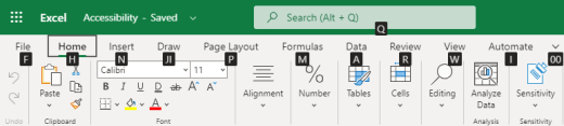
-
To get to the ribbon, press Alt+Windows logo key, or press Ctrl+F6 until you reach the Home tab.
-
To move between tabs on the ribbon, press the Tab key.
-
To hide the ribbon so you have more room to work, press Ctrl+F1. To display the ribbon again, press Ctrl+F1.
Go to the access keys for the ribbon
To go directly to a tab on the ribbon, press one of the following access keys:
|
To do this |
Press |
|---|---|
|
Go to the Search or Tell Me field on the ribbon and type a search term. |
Alt+Windows logo key, Q |
|
Open the File menu. |
Alt+Windows logo key, F |
|
Open the Home tab and format text and numbers or use other tools such as Sort & Filter. |
Alt+Windows logo key, H |
|
Open the Insert tab and insert a function, table, chart, hyperlink, or threaded comment. |
Alt+Windows logo key, N |
|
Open the Data tab and refresh connections or use data tools. |
Alt+Windows logo key, A |
|
Open the Review tab and use the Accessibility Checker or work with threaded comments and notes. |
Alt+Windows logo key, R |
|
Open the View tab to choose a view, freeze rows or columns in your worksheet, or show gridlines and headers. |
Alt+Windows logo key, W |
Top of Page
Work in the ribbon tabs and menus
The shortcuts in this table can save time when you work with the ribbon tabs and ribbon menus.
|
To do this |
Press |
|---|---|
|
Select the active tab of the ribbon and activate the access keys. |
Alt+Windows logo key. To move to a different tab, use an access key or the Tab key. |
|
Move the focus to commands on the ribbon. |
Enter, then the Tab key or Shift+Tab |
|
Activate a selected button. |
Spacebar or Enter |
|
Open the list for a selected command. |
Spacebar or Enter |
|
Open the menu for a selected button. |
Alt+Down arrow key |
|
When a menu or submenu is open, move to the next command. |
Esc |
Top of Page
Keyboard shortcuts for editing cells
Tip: If a spreadsheet opens in the Viewing mode, editing commands won’t work. To switch to Editing mode, press Alt+Windows logo key, Z, M, E.
|
To do this |
Press |
|---|---|
|
Insert a row above the current row. |
Alt+Windows logo key, H, I, R |
|
Insert a column to the left of the current column. |
Alt+Windows logo key, H, I, C |
|
Cut selection. |
Ctrl+X |
|
Copy selection. |
Ctrl+C |
|
Paste selection. |
Ctrl+V |
|
Undo an action. |
Ctrl+Z |
|
Redo an action. |
Ctrl+Y |
|
Start a new line in the same cell. |
Alt+Enter |
|
Insert a hyperlink. |
Ctrl+K |
|
Insert a table. |
Ctrl+L |
|
Insert a function. |
Shift+F3 |
|
Increase font size. |
Ctrl+Shift+Right angle bracket (>) |
|
Decrease font size. |
Ctrl+Shift+Left angle bracket (<) |
|
Apply a filter. |
Alt+Windows logo key, A, T |
|
Re-apply a filter. |
Ctrl+Alt+L |
|
Toggle AutoFilter on and off. |
Ctrl+Shift+L |
Top of Page
Keyboard shortcuts for entering data
|
To do this |
Press |
|---|---|
|
Complete cell entry and select the cell below. |
Enter |
|
Complete cell entry and select the cell above. |
Shift+Enter |
|
Complete cell entry and select the next cell in the row. |
Tab key |
|
Complete cell entry and select the previous cell in the row. |
Shift+Tab |
|
Cancel cell entry. |
Esc |
Top of Page
Keyboard shortcuts for editing data within a cell
|
To do this |
Press |
|---|---|
|
Edit the selected cell. |
F2 |
|
Cycle through all the various combinations of absolute and relative references when a cell reference or range is selected in a formula. |
F4 |
|
Clear the selected cell. |
Delete |
|
Clear the selected cell and start editing. |
Backspace |
|
Go to beginning of cell line. |
Home |
|
Go to end of cell line. |
End |
|
Select right by one character. |
Shift+Right arrow key |
|
Select to the beginning of cell data. |
Shift+Home |
|
Select to the end of cell data. |
Shift+End |
|
Select left by one character. |
Shift+Left arrow key |
|
Extend selection to the last nonblank cell in the same column or row as the active cell, or if the next cell is blank, to the next nonblank cell. |
Ctrl+Shift+Right arrow key or Ctrl+Shift+Left arrow key |
|
Insert the current date. |
Ctrl+Semicolon (;) |
|
Insert the current time. |
Ctrl+Shift+Semicolon (;) |
|
Copy a formula from the cell above. |
Ctrl+Apostrophe (‘) |
|
Copy the value from the cell above. |
Ctrl+Shift+Apostrophe (‘) |
|
Insert a formula argument. |
Ctrl+Shift+A |
Top of Page
Keyboard shortcuts for formatting cells
|
To do this |
Press |
|---|---|
|
Apply bold formatting. |
Ctrl+B |
|
Apply italic formatting. |
Ctrl+I |
|
Apply underline formatting. |
Ctrl+U |
|
Paste formatting. |
Shift+Ctrl+V |
|
Apply the outline border to the selected cells. |
Ctrl+Shift+Ampersand (&) |
|
Apply the number format. |
Ctrl+Shift+1 |
|
Apply the time format. |
Ctrl+Shift+2 |
|
Apply the date format. |
Ctrl+Shift+3 |
|
Apply the currency format. |
Ctrl+Shift+4 |
|
Apply the percentage format. |
Ctrl+Shift+5 |
|
Apply the scientific format. |
Ctrl+Shift+6 |
|
Apply outside border. |
Ctrl+Shift+7 |
|
Open the Number Format dialog box. |
Ctrl+1 |
Top of Page
Keyboard shortcuts for moving and scrolling within worksheets
|
To do this |
Press |
|---|---|
|
Move up one cell. |
Up arrow key or Shift+Enter |
|
Move down one cell. |
Down arrow key or Enter |
|
Move right one cell. |
Right arrow key or Tab key |
|
Go to the beginning of the row. |
Home |
|
Go to cell A1. |
Ctrl+Home |
|
Go to the last cell of the used range. |
Ctrl+End |
|
Move down one screen (28 rows). |
Page down |
|
Move up one screen (28 rows). |
Page up |
|
Move to the edge of the current data region. |
Ctrl+Right arrow key or Ctrl+Left arrow key |
|
Move between ribbon and workbook content. |
Ctrl+F6 |
|
Move to a different ribbon tab. |
Tab key Press Enter to go to the ribbon for the tab. |
|
Insert a new sheet. |
Shift+F11 |
|
Switch to the next sheet. |
Alt+Ctrl+Page down |
|
Switch to the next sheet (when in Microsoft Teams or a browser other than Chrome). |
Ctrl+Page down |
|
Switch to the previous sheet. |
Alt+Ctrl+Page up |
|
Switch to previous sheet (when in Microsoft Teams or a browser other than Chrome). |
Ctrl+Page up |
Top of Page
Keyboard shortcuts for working with objects
|
To do this |
Press |
|---|---|
|
Open menu or drill down. |
Alt+Down arrow key |
|
Close menu or drill up. |
Alt+Up arrow key |
|
Follow hyperlink. |
Ctrl+Enter |
|
Open a note for editing. |
Shift+F2 |
|
Open and reply to a threaded comment. |
Ctrl+Shift+F2 |
|
Rotate an object left. |
Alt+Left arrow key |
|
Rotate an object right. |
Alt+Right arrow key |
Top of Page
Keyboard shortcuts for working with cells, rows, columns, and objects
|
To do this |
Press |
|---|---|
|
Select a range of cells. |
Shift+Arrow keys |
|
Select an entire column. |
Ctrl+Spacebar |
|
Select an entire row. |
Shift+Spacebar |
|
Extend selection to the last nonblank cell in the same column or row as the active cell, or if the next cell is blank, to the next nonblank cell. |
Ctrl+Shift+Right arrow key or Ctrl+Shift+Left arrow key |
|
Add a non-adjacent cell or range to a selection. |
Shift+F8 |
|
Insert cells, rows, or columns. |
Ctrl+Plus sign (+) |
|
Delete cells, rows, or columns. |
Ctrl+Minus sign (-) |
|
Hide rows. |
Ctrl+9 |
|
Unhide rows. |
Ctrl+Shift+9 |
|
Hide columns |
Ctrl+0 |
|
Unhide columns |
Ctrl+Shift+0 |
Top of Page
Keyboard shortcuts for moving within a selected range
|
To do this |
Press |
|---|---|
|
Move from top to bottom (or forward through the selection). |
Enter |
|
Move from bottom to top (or back through the selection). |
Shift+Enter |
|
Move forward through a row (or down through a single-column selection). |
Tab key |
|
Move back through a row (or up through a single-column selection). |
Shift+Tab |
|
Move to an active cell. |
Shift+Backspace |
|
Move to an active cell and keep the selection. |
Ctrl+Backspace |
|
Rotate the active cell through the corners of the selection. |
Ctrl+Period (.) |
|
Move to the next selected range. |
Ctrl+Alt+Right arrow key |
|
Move to the previous selected range. |
Ctrl+Alt+Left arrow key |
|
Extend selection to the last used cell in the sheet. |
Ctrl+Shift+End |
|
Extend selection to the first cell in the sheet. |
Ctrl+Shift+Home |
Top of Page
Keyboard shortcuts for calculating data
|
To do this |
Press |
|---|---|
|
Calculate workbook (refresh). |
F9 |
|
Perform full calculation. |
Ctrl+Shift+Alt+F9 |
|
Refresh external data. |
Alt+F5 |
|
Refresh all external data. |
Ctrl+Alt+F5 |
|
Apply Auto Sum. |
Alt+Equal sign ( = ) |
|
Apply Flash Fill. |
Ctrl+E |
Top of Page
Accessibility Shortcuts Menu (Alt+Shift+A)
Access the common features quickly by using the following shortcuts:
|
To do this |
Press |
|---|---|
|
Cycle between landmark regions. |
Ctrl+F6 or Ctrl+Shift+F6 |
|
Move within a landmark region. |
Tab key or Shift+Tab |
|
Go to the Search or Tell Me field to run any command. |
Alt+Q |
|
Display or hide Key Tips or access the ribbon. |
Alt+Windows logo key |
|
Edit the selected cell. |
F2 |
|
Go to a specific cell. |
Ctrl+G |
|
Move to another worksheet in the workbook. |
Ctrl+Alt+Page up or Ctrl+Alt+Page down |
|
Open the context menu. |
Shift+F10 or Windows Menu key |
|
Read row header. |
Ctrl+Alt+Shift+T |
|
Read row until an active cell. |
Ctrl+Alt+Shift+Home |
|
Read row from an active cell. |
Ctrl+Alt+Shift+End |
|
Read column header. |
Ctrl+Alt+Shift+H |
|
Read column until an active cell. |
Ctrl+Alt+Shift+Page up |
|
Read column from an active cell. |
Ctrl+Alt+Shift+Page down |
|
Open a list of moving options within a dialog box. |
Ctrl+Alt+Spacebar |
Top of Page
Control keyboard shortcuts in Excel for the web by overriding browser keyboard shortcuts
Excel for the web works in a browser. Browsers have keyboard shortcuts, some of which conflict with shortcuts that work in Excel on the desktop. You can control these shortcuts, so they work the same in both versions of Excel by changing the Keyboard Shortcuts settings. Overriding browser shortcuts also enables you to open the Excel for the web Help by pressing F1.
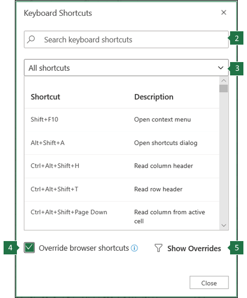
|
|
Top of Page
See also
Excel help & learning
Use a screen reader to explore and navigate Excel
Basic tasks using a screen reader with Excel
Screen reader support for Excel
Technical support for customers with disabilities
Microsoft wants to provide the best possible experience for all our customers. If you have a disability or questions related to accessibility, please contact the Microsoft Disability Answer Desk for technical assistance. The Disability Answer Desk support team is trained in using many popular assistive technologies and can offer assistance in English, Spanish, French, and American Sign Language. Please go to the Microsoft Disability Answer Desk site to find out the contact details for your region.
If you are a government, commercial, or enterprise user, please contact the enterprise Disability Answer Desk.
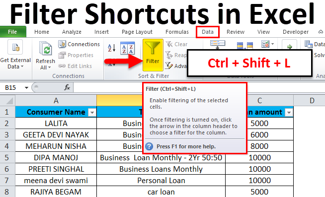
Excel Filter Shortcuts (Table of Contents)
- Filter Shortcuts in Excel
- How to Use Filter Shortcut in Excel?
Filter Shortcuts in Excel
There are different ways to access and apply Filter in Excel. In a first way, we can select the headers first, then from the Data menu tab, select Filter Option, which is under the Sort & Filter section. In a second way, we can apply the filter by pressing short cut keys Alt + D + F + F simultaneously, and another way is by pressing short cut keys Shift + Ctrl + L together to apply a filter in one go. Once the filter is applied, we can use other short cut keys such as the Alt + Down key to get into the applied filter and select an option either by pressing a shortcut key or navigation keys.
How to Use Filter Shortcut in Excel?
Filter Shortcut in Excel is very simple and easy to use. Let’s understand the working of filter shortcut in excel with some examples.
You can download this Filter Shortcuts Excel Template here – Filter Shortcuts Excel Template
#1 – Toggle Autofilter in the ribbon
Example #1
Here is a sample data on which we have to apply a filter.
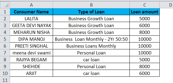
- We have to first click on the Data tab and then click on Filter, as shown below.
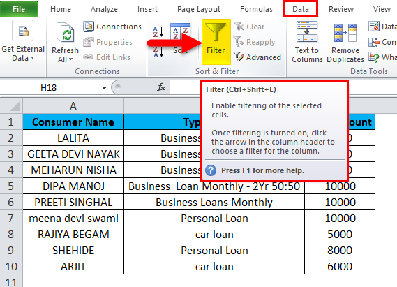
- Once we click the Filter tab on the ribbon, we will see that filter is applied to the data, that is, on all the columns.
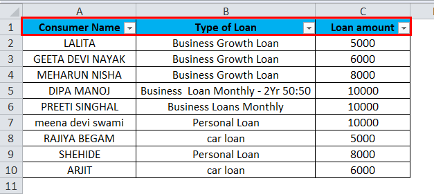
- Now, if we want to see the name of consumers who have taken Business Growth Loan, we can select Business Growth Loan in the filter drop-down and then click on OK as shown below:
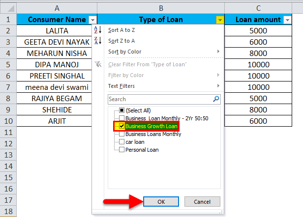
- You will see the name of the consumers who have taken Business Growth Loan.
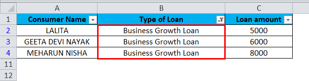
- To disable Filter, you just need to again click on the Filter in Ribbon in MS Excel.
Example #2
- Now, if we want to see how many consumers have taken a loan of 10000, we can apply the filter as shown below:
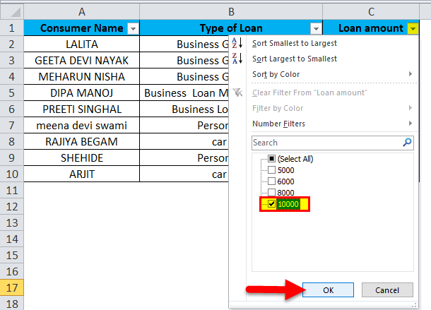
- On clicking Ok. You will then be able to filter the data as per your requirement.
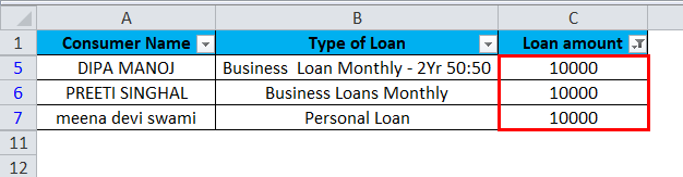
#2 – Applying filter using “Sort and Filter” option on the Home tab in the Editing Group
It can be found on the right side of the Ribbon in MS Excel.
Using the above data, here is how we can apply the filter:
- To apply a filter, click on Sort & Filter, then click on the Filter option, which is the fourth option in the dropdown.
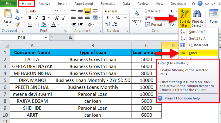
Example #3
- To filter the consumers who have taken a car loan.
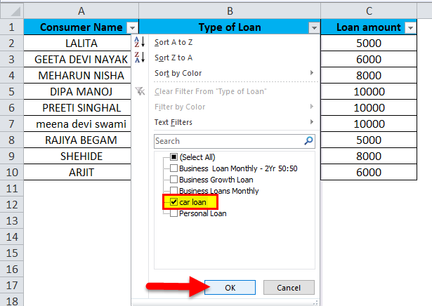
- On clicking Ok. You will see the consumers who have taken a car loan.
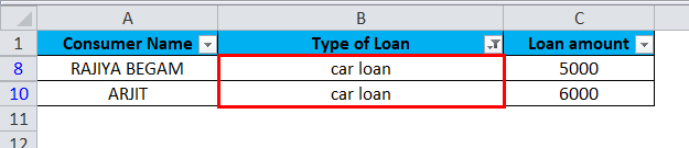
Example #4
Now, if we need to filter some particular consumers, like their loan amount and their loan type, suppose we want to know the above details for Arjit and Dipa; we will apply the filter as below:
- Now select Arjit and Dipa Manoj in the filter dropdown and then click on Ok.
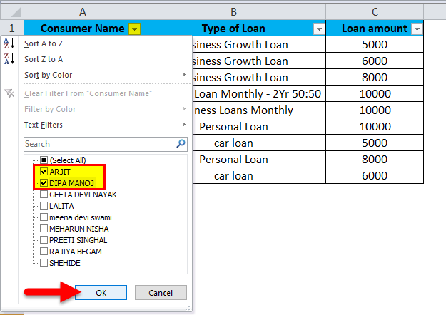
- We will then be able to see the relevant details.
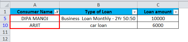
- You can disable the filter on the data by clicking on the Sort and Filter option.
#3 – Filter the Excel data by shortcut key
We can rapidly press a shortcut key to apply the filter in our data. Together, we have to press Ctrl+shift+L.
Example #5
Here is a sample data on which we have applied the filter using the shortcut key.
- Select the data and then press the shortcut key to apply the filter, i.e. Ctrl+shift+L.
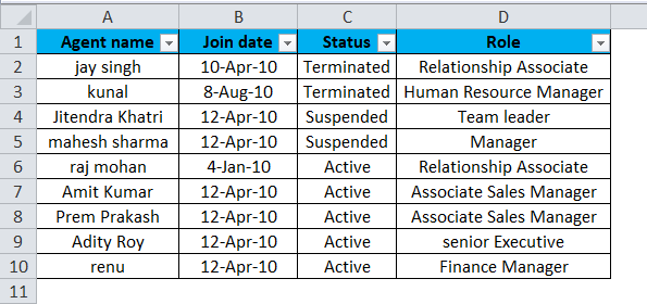
- If we want to filter the status of the Agents, like Active and Terminated, from the complete data, we will proceed as below:
- Press OK, and we will see the Active and Terminated agents.
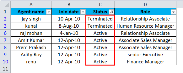
While applying filters on the selected criteria, we see other options as well as shown below:
On top of the filter drop-down, we see an option Sort A to Z; then we have Sort Z to A, Sort by color and Text filters.
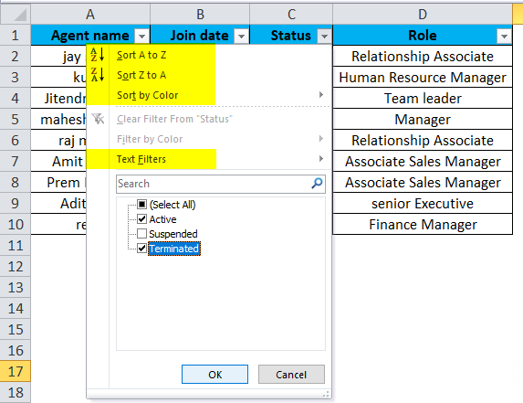
Let’s look into these options. If we click on Sort A to Z, this is how we see the data:
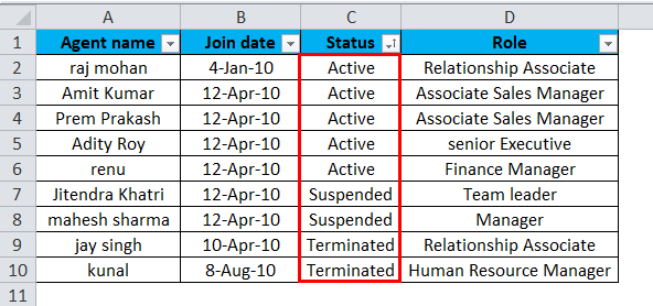
The data is filtered and got sorted in order of A to Z. Likewise, if we click Sort Z to A, we will see the data as below:
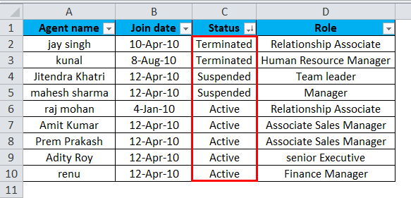
The data is filtered and also got sorted in order of Z to A.
By clicking Sort by color, the data will be filtered as per our criteria and will also be sorted as per color of that cell, like if you select a cell colored red that will be on the top.
And, if we click Text Filter:
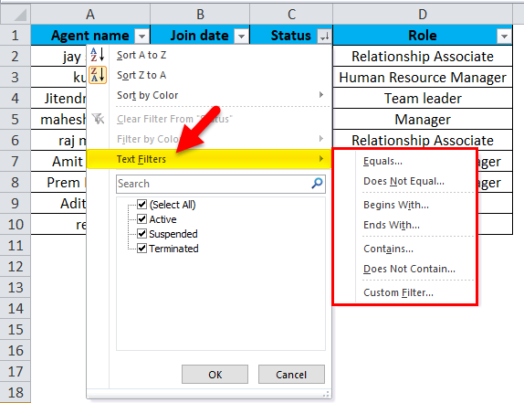
We get an option for an advanced filter for text, such as:
- Filter cells that Begin with or End with a specific text or character.
- Filter cells that Contain or Does not Contain a specific text or character.
- Filter cells that are either Equals to or Does not equal to a specific text or characters.
When we click on Does not equal to option and write Suspended in the dialogue box as shown below:
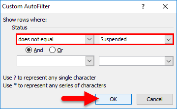
After we click “Ok”, we will see the data filtered as:
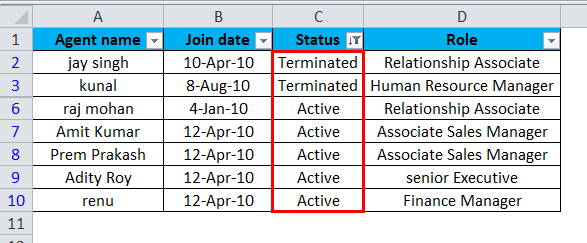
The data shows only Active and terminated status and not suspended.
Once you have applied the filter, you can disable it from that column as shown:
- Once we click Clear Filter from “Status”, the filter will be cleared from the Status column of the data.
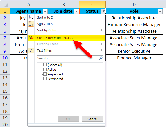
To remove a filter from the whole data, again press Ctrl+Shift+L.
Once you have filtered the data, you can copy it to any other worksheet or workbook. You can do this by selecting the filtered data or filtered cells by pressing Ctrl + A . Then Press Ctrl+C to copy the filtered data and go to another worksheet/workbook and paste the filtered data by pressing Ctrl+V.
Things to Remember about Filter Shortcuts in Excel
- Some Excel filters can be used one at a time. For Example, you can filter a column by either value or color at a time and not with both the options simultaneously.
- For better results, avoid using different value types in a column as for one column, one filter type is available. If a column contains different types of values, the filter will be applied for the data that has a high frequency. For example, if the data is in number in a column but is formatted as text, then the text filter will be applied and not the number filter.
- Once you have filtered a column and pasted the data, remove a filter from that column because the next filter in a different column will not take into account that filter, and hence the filtered data will be correct.
Recommended Articles
This has been a guide to Filter Shortcuts in Excel. Here we discuss how to use filter shortcuts in Excel along with practical examples and a downloadable excel template. You can also go through our other suggested articles –
- Advanced Filter in Excel
- AutoFilter in Excel
- Adding Data Filter in Excel
- VBA Filter