Shortcuts and formulas of excel - Word и Excel - помощь в работе с программами

Many users find that using an external keyboard with keyboard shortcuts for Excel helps them work more efficiently. For users with mobility or vision disabilities, keyboard shortcuts can be easier than using the touchscreen and are an essential alternative to using a mouse.

Notes:

The shortcuts in this topic refer to the US keyboard layout. Keys for other layouts might not correspond exactly to the keys on a US keyboard.
A plus sign (+) in a shortcut means that you need to press multiple keys at the same time.
A comma sign (,) in a shortcut means that you need to press multiple keys in order.

This article describes the keyboard shortcuts, function keys, and some other common shortcut keys in Excel for Windows.

Notes:

To quickly find a shortcut in this article, you can use the Search. Press Ctrl+F, and then type your search words.
If an action that you use often does not have a shortcut key, you can record a macro to create one. For instructions, go to Automate tasks with the Macro Recorder.
Download our 50 time-saving Excel shortcuts quick tips guide.
Get the Excel 2016 keyboard shortcuts in a Word document: Excel keyboard shortcuts and function keys.

In this topic

Frequently used shortcuts
Ribbon keyboard shortcuts
- Use the Access keys for ribbon tabs
- Work in the ribbon with the keyboard
Keyboard shortcuts for navigating in cells
Keyboard shortcuts for formatting cells
- Keyboard shortcuts in the Paste Special dialog box in Excel 2013
Keyboard shortcuts for making selections and performing actions
Keyboard shortcuts for working with data, functions, and the formula bar
Keyboard shortcuts for refreshing external data
Power Pivot keyboard shortcuts
Function keys
Other useful shortcut keys

Frequently used shortcuts

This table lists the most frequently used shortcuts in Excel.

To do this	Press
Close a workbook.	Ctrl+W
Open a workbook.	Ctrl+O
Go to the Home tab.	Alt+H
Save a workbook.	Ctrl+S
Copy selection.	Ctrl+C
Paste selection.	Ctrl+V
Undo recent action.	Ctrl+Z
Remove cell contents.	Delete
Choose a fill color.	Alt+H, H
Cut selection.	Ctrl+X
Go to the Insert tab.	Alt+N
Apply bold formatting.	Ctrl+B
Center align cell contents.	Alt+H, A, C
Go to the Page Layout tab.	Alt+P
Go to the Data tab.	Alt+A
Go to the View tab.	Alt+W
Open the context menu.	Shift+F10 or Windows Menu key
Add borders.	Alt+H, B
Delete column.	Alt+H, D, C
Go to the Formula tab.	Alt+M
Hide the selected rows.	Ctrl+9
Hide the selected columns.	Ctrl+0

Top of Page

Ribbon keyboard shortcuts

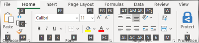
The ribbon groups related options on tabs. For example, on the Home tab, the Number group includes the Number Format option. Press the Alt key to display the ribbon shortcuts, called Key Tips, as letters in small images next to the tabs and options as shown in the image below.

You can combine the Key Tips letters with the Alt key to make shortcuts called Access Keys for the ribbon options. For example, press Alt+H to open the Home tab, and Alt+Q to move to the Tell me or Search field. Press Alt again to see KeyTips for the options for the selected tab.

Depending on the version of Microsoft 365 you are using, the Search text field at the top of the app window might be called Tell Me instead. Both offer a largely similar experience, but some options and search results can vary.

In Office 2013 and Office 2010, most of the old Alt key menu shortcuts still work, too. However, you need to know the full shortcut. For example, press Alt, and then press one of the old menu keys, for example, E (Edit), V (View), I (Insert), and so on. A notification pops up saying you’re using an access key from an earlier version of Microsoft 365. If you know the entire key sequence, go ahead, and use it. If you don’t know the sequence, press Esc and use Key Tips instead.

Use the Access keys for ribbon tabs

To go directly to a tab on the ribbon, press one of the following access keys. Additional tabs might appear depending on your selection in the worksheet.

To do this	Press
Move to the Tell me or Search field on the ribbon and type a search term for assistance or Help content.	Alt+Q, then enter the search term.
Open the File menu.	Alt+F
Open the Home tab and format text and numbers and use the Find tool.	Alt+H
Open the Insert tab and insert PivotTables, charts, add-ins, Sparklines, pictures, shapes, headers, or text boxes.	Alt+N
Open the Page Layout tab and work with themes, page setup, scale, and alignment.	Alt+P
Open the Formulas tab and insert, trace, and customize functions and calculations.	Alt+M
Open the Data tab and connect to, sort, filter, analyze, and work with data.	Alt+A
Open the Review tab and check spelling, add notes and threaded comments, and protect sheets and workbooks.	Alt+R
Open the View tab and preview page breaks and layouts, show and hide gridlines and headings, set zoom magnification, manage windows and panes, and view macros.	Alt+W

Top of Page

Work in the ribbon with the keyboard

To do this	Press
Select the active tab on the ribbon and activate the access keys.	Alt or F10. To move to a different tab, use access keys or the arrow keys.
Move the focus to commands on the ribbon.	Tab key or Shift+Tab
Move down, up, left, or right, respectively, among the items on the ribbon.	Arrow keys
Show the tooltip for the ribbon element currently in focus.	Ctrl+Shift+F10
Activate a selected button.	Spacebar or Enter
Open the list for a selected command.	Down arrow key
Open the menu for a selected button.	Alt+Down arrow key
When a menu or submenu is open, move to the next command.	Down arrow key
Expand or collapse the ribbon.	Ctrl+F1
Open a context menu.	Shift+F10 Or, on a Windows keyboard, the Windows Menu key (usually between the Alt Gr and right Ctrl keys)
Move to the submenu when a main menu is open or selected.	Left arrow key
Move from one group of controls to another.	Ctrl+Left or Right arrow key

Top of Page

Keyboard shortcuts for navigating in cells

To do this	Press
Move to the previous cell in a worksheet or the previous option in a dialog box.	Shift+Tab
Move one cell up in a worksheet.	Up arrow key
Move one cell down in a worksheet.	Down arrow key
Move one cell left in a worksheet.	Left arrow key
Move one cell right in a worksheet.	Right arrow key
Move to the edge of the current data region in a worksheet.	Ctrl+Arrow key
Enter the End mode, move to the next nonblank cell in the same column or row as the active cell, and turn off End mode. If the cells are blank, move to the last cell in the row or column.	End, Arrow key
Move to the last cell on a worksheet, to the lowest used row of the rightmost used column.	Ctrl+End
Extend the selection of cells to the last used cell on the worksheet (lower-right corner).	Ctrl+Shift+End
Move to the cell in the upper-left corner of the window when Scroll lock is turned on.	Home+Scroll lock
Move to the beginning of a worksheet.	Ctrl+Home
Move one screen down in a worksheet.	Page down
Move to the next sheet in a workbook.	Ctrl+Page down
Move one screen to the right in a worksheet.	Alt+Page down
Move one screen up in a worksheet.	Page up
Move one screen to the left in a worksheet.	Alt+Page up
Move to the previous sheet in a workbook.	Ctrl+Page up
Move one cell to the right in a worksheet. Or, in a protected worksheet, move between unlocked cells.	Tab key
Open the list of validation choices on a cell that has data validation option applied to it.	Alt+Down arrow key
Cycle through floating shapes, such as text boxes or images.	Ctrl+Alt+5, then the Tab key repeatedly
Exit the floating shape navigation and return to the normal navigation.	Esc
Scroll horizontally.	Ctrl+Shift, then scroll your mouse wheel up to go left, down to go right
Zoom in.	Ctrl+Alt+Equal sign ( = )
Zoom out.	Ctrl+Alt+Minus sign (-)

Top of Page

Keyboard shortcuts for formatting cells

To do this	Press
Open the Format Cells dialog box.	Ctrl+1
Format fonts in the Format Cells dialog box.	Ctrl+Shift+F or Ctrl+Shift+P
Edit the active cell and put the insertion point at the end of its contents. Or, if editing is turned off for the cell, move the insertion point into the formula bar. If editing a formula, toggle Point mode off or on so you can use the arrow keys to create a reference.	F2
Insert a note. Open and edit a cell note.	Shift+F2 Shift+F2
Insert a threaded comment. Open and reply to a threaded comment.	Ctrl+Shift+F2 Ctrl+Shift+F2
Open the Insert dialog box to insert blank cells.	Ctrl+Shift+Plus sign (+)
Open the Delete dialog box to delete selected cells.	Ctrl+Minus sign (-)
Enter the current time.	Ctrl+Shift+Colon (:)
Enter the current date.	Ctrl+Semicolon (;)
Switch between displaying cell values or formulas in the worksheet.	Ctrl+Grave accent (`)
Copy a formula from the cell above the active cell into the cell or the formula bar.	Ctrl+Apostrophe (‘)
Move the selected cells.	Ctrl+X
Copy the selected cells.	Ctrl+C
Paste content at the insertion point, replacing any selection.	Ctrl+V
Open the Paste Special dialog box.	Ctrl+Alt+V
Italicize text or remove italic formatting.	Ctrl+I or Ctrl+3
Bold text or remove bold formatting.	Ctrl+B or Ctrl+2
Underline text or remove underline.	Ctrl+U or Ctrl+4
Apply or remove strikethrough formatting.	Ctrl+5
Switch between hiding objects, displaying objects, and displaying placeholders for objects.	Ctrl+6
Apply an outline border to the selected cells.	Ctrl+Shift+Ampersand sign (&)
Remove the outline border from the selected cells.	Ctrl+Shift+Underscore (_)
Display or hide the outline symbols.	Ctrl+8
Use the Fill Down command to copy the contents and format of the topmost cell of a selected range into the cells below.	Ctrl+D
Apply the General number format.	Ctrl+Shift+Tilde sign (~)
Apply the Currency format with two decimal places (negative numbers in parentheses).	Ctrl+Shift+Dollar sign ($)
Apply the Percentage format with no decimal places.	Ctrl+Shift+Percent sign (%)
Apply the Scientific number format with two decimal places.	Ctrl+Shift+Caret sign (^)
Apply the Date format with the day, month, and year.	Ctrl+Shift+Number sign (#)
Apply the Time format with the hour and minute, and AM or PM.	Ctrl+Shift+At sign (@)
Apply the Number format with two decimal places, thousands separator, and minus sign (-) for negative values.	Ctrl+Shift+Exclamation point (!)
Open the Insert hyperlink dialog box.	Ctrl+K
Check spelling in the active worksheet or selected range.	F7
Display the Quick Analysis options for selected cells that contain data.	Ctrl+Q
Display the Create Table dialog box.	Ctrl+L or Ctrl+T
Open the Workbook Statistics dialog box.	Ctrl+Shift+G

Top of Page

Keyboard shortcuts in the Paste Special dialog box in Excel 2013

In Excel 2013, you can paste a specific aspect of the copied data like its formatting or value using the Paste Special options. After you’ve copied the data, press Ctrl+Alt+V, or Alt+E+S to open the Paste Special dialog box.

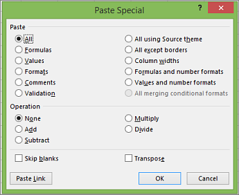
Tip: You can also select Home > Paste > Paste Special.

To pick an option in the dialog box, press the underlined letter for that option. For example, press the letter C to pick the Comments option.

To do this	Press
Paste all cell contents and formatting.	A
Paste only the formulas as entered in the formula bar.	F
Paste only the values (not the formulas).	V
Paste only the copied formatting.	T
Paste only comments and notes attached to the cell.	C
Paste only the data validation settings from copied cells.	N
Paste all cell contents and formatting from copied cells.	H
Paste all cell contents without borders.	X
Paste only column widths from copied cells.	W
Paste only formulas and number formats from copied cells.	R
Paste only the values (not formulas) and number formats from copied cells.	U

Top of Page

Keyboard shortcuts for making selections and performing actions

To do this	Press
Select the entire worksheet.	Ctrl+A or Ctrl+Shift+Spacebar
Select the current and next sheet in a workbook.	Ctrl+Shift+Page down
Select the current and previous sheet in a workbook.	Ctrl+Shift+Page up
Extend the selection of cells by one cell.	Shift+Arrow key
Extend the selection of cells to the last nonblank cell in the same column or row as the active cell, or if the next cell is blank, to the next nonblank cell.	Ctrl+Shift+Arrow key
Turn extend mode on and use the arrow keys to extend a selection. Press again to turn off.	F8
Add a non-adjacent cell or range to a selection of cells by using the arrow keys.	Shift+F8
Start a new line in the same cell.	Alt+Enter
Fill the selected cell range with the current entry.	Ctrl+Enter
Complete a cell entry and select the cell above.	Shift+Enter
Select an entire column in a worksheet.	Ctrl+Spacebar
Select an entire row in a worksheet.	Shift+Spacebar
Select all objects on a worksheet when an object is selected.	Ctrl+Shift+Spacebar
Extend the selection of cells to the beginning of the worksheet.	Ctrl+Shift+Home
Select the current region if the worksheet contains data. Press a second time to select the current region and its summary rows. Press a third time to select the entire worksheet.	Ctrl+A or Ctrl+Shift+Spacebar
Select the current region around the active cell.	Ctrl+Shift+Asterisk sign (*)
Select the first command on the menu when a menu or submenu is visible.	Home
Repeat the last command or action, if possible.	Ctrl+Y
Undo the last action.	Ctrl+Z
Expand grouped rows or columns.	While hovering over the collapsed items, press and hold the Shift key and scroll down.
Collapse grouped rows or columns.	While hovering over the expanded items, press and hold the Shift key and scroll up.

Top of Page

Keyboard shortcuts for working with data, functions, and the formula bar

To do this	Press
Turn on or off tooltips for checking formulas directly in the formula bar or in the cell you’re editing.	Ctrl+Alt+P
Edit the active cell and put the insertion point at the end of its contents. Or, if editing is turned off for the cell, move the insertion point into the formula bar. If editing a formula, toggle Point mode off or on so you can use the arrow keys to create a reference.	F2
Expand or collapse the formula bar.	Ctrl+Shift+U
Cancel an entry in the cell or formula bar.	Esc
Complete an entry in the formula bar and select the cell below.	Enter
Move the cursor to the end of the text when in the formula bar.	Ctrl+End
Select all text in the formula bar from the cursor position to the end.	Ctrl+Shift+End
Calculate all worksheets in all open workbooks.	F9
Calculate the active worksheet.	Shift+F9
Calculate all worksheets in all open workbooks, regardless of whether they have changed since the last calculation.	Ctrl+Alt+F9
Check dependent formulas, and then calculate all cells in all open workbooks, including cells not marked as needing to be calculated.	Ctrl+Alt+Shift+F9
Display the menu or message for an Error Checking button.	Alt+Shift+F10
Display the Function Arguments dialog box when the insertion point is to the right of a function name in a formula.	Ctrl+A
Insert argument names and parentheses when the insertion point is to the right of a function name in a formula.	Ctrl+Shift+A
Insert the AutoSum formula	Alt+Equal sign ( = )
Invoke Flash Fill to automatically recognize patterns in adjacent columns and fill the current column	Ctrl+E
Cycle through all combinations of absolute and relative references in a formula if a cell reference or range is selected.	F4
Insert a function.	Shift+F3
Copy the value from the cell above the active cell into the cell or the formula bar.	Ctrl+Shift+Straight quotation mark («)
Create an embedded chart of the data in the current range.	Alt+F1
Create a chart of the data in the current range in a separate Chart sheet.	F11
Define a name to use in references.	Alt+M, M, D
Paste a name from the Paste Name dialog box (if names have been defined in the workbook).	F3
Move to the first field in the next record of a data form.	Enter
Create, run, edit, or delete a macro.	Alt+F8
Open the Microsoft Visual Basic For Applications Editor.	Alt+F11
Open the Power Query Editor	Alt+F12

Top of Page

Keyboard shortcuts for refreshing external data

Use the following keys to refresh data from external data sources.

To do this	Press
Stop a refresh operation.	Esc
Refresh data in the current worksheet.	Ctrl+F5
Refresh all data in the workbook.	Ctrl+Alt+F5

Top of Page

Power Pivot keyboard shortcuts

Use the following keyboard shortcuts with Power Pivot in Microsoft 365, Excel 2019, Excel 2016, and Excel 2013.

To do this	Press
Open the context menu for the selected cell, column, or row.	Shift+F10
Select the entire table.	Ctrl+A
Copy selected data.	Ctrl+C
Delete the table.	Ctrl+D
Move the table.	Ctrl+M
Rename the table.	Ctrl+R
Save the file.	Ctrl+S
Redo the last action.	Ctrl+Y
Undo the last action.	Ctrl+Z
Select the current column.	Ctrl+Spacebar
Select the current row.	Shift+Spacebar
Select all cells from the current location to the last cell of the column.	Shift+Page down
Select all cells from the current location to the first cell of the column.	Shift+Page up
Select all cells from the current location to the last cell of the row.	Shift+End
Select all cells from the current location to the first cell of the row.	Shift+Home
Move to the previous table.	Ctrl+Page up
Move to the next table.	Ctrl+Page down
Move to the first cell in the upper-left corner of selected table.	Ctrl+Home
Move to the last cell in the lower-right corner of selected table.	Ctrl+End
Move to the first cell of the selected row.	Ctrl+Left arrow key
Move to the last cell of the selected row.	Ctrl+Right arrow key
Move to the first cell of the selected column.	Ctrl+Up arrow key
Move to the last cell of selected column.	Ctrl+Down arrow key
Close a dialog box or cancel a process, such as a paste operation.	Ctrl+Esc
Open the AutoFilter Menu dialog box.	Alt+Down arrow key
Open the Go To dialog box.	F5
Recalculate all formulas in the Power Pivot window. For more information, see Recalculate Formulas in Power Pivot.	F9

Top of Page

Function keys

Key	Description
F1	F1 alone: displays the Excel Help task pane. Ctrl+F1: displays or hides the ribbon. Alt+F1: creates an embedded chart of the data in the current range. Alt+Shift+F1: inserts a new worksheet. Ctrl+Shift+F1: toggles full screen mode
F2	F2 alone: edit the active cell and put the insertion point at the end of its contents. Or, if editing is turned off for the cell, move the insertion point into the formula bar. If editing a formula, toggle Point mode off or on so you can use the arrow keys to create a reference. Shift+F2: adds or edits a cell note. Ctrl+F2: displays the print preview area on the Print tab in the Backstage view.
F3	F3 alone: displays the Paste Name dialog box. Available only if names have been defined in the workbook. Shift+F3: displays the Insert Function dialog box.
F4	F4 alone: repeats the last command or action, if possible. When a cell reference or range is selected in a formula, F4 cycles through all the various combinations of absolute and relative references. Ctrl+F4: closes the selected workbook window. Alt+F4: closes Excel.
F5	F5 alone: displays the Go To dialog box. Ctrl+F5: restores the window size of the selected workbook window.
F6	F6 alone: switches between the worksheet, ribbon, task pane, and Zoom controls. In a worksheet that has been split, F6 includes the split panes when switching between panes and the ribbon area. Shift+F6: switches between the worksheet, Zoom controls, task pane, and ribbon. Ctrl+F6: switches between two Excel windows. Ctrl+Shift+F6: switches between all Excel windows.
F7	F7 alone: Opens the Spelling dialog box to check spelling in the active worksheet or selected range. Ctrl+F7: performs the Move command on the workbook window when it is not maximized. Use the arrow keys to move the window, and when finished press Enter, or Esc to cancel.
F8	F8 alone: turns extend mode on or off. In extend mode, Extended Selection appears in the status line, and the arrow keys extend the selection. Shift+F8: enables you to add a non-adjacent cell or range to a selection of cells by using the arrow keys. Ctrl+F8: performs the Size command when a workbook is not maximized. Alt+F8: displays the Macro dialog box to create, run, edit, or delete a macro.
F9	F9 alone: calculates all worksheets in all open workbooks. Shift+F9: calculates the active worksheet. Ctrl+Alt+F9: calculates all worksheets in all open workbooks, regardless of whether they have changed since the last calculation. Ctrl+Alt+Shift+F9: rechecks dependent formulas, and then calculates all cells in all open workbooks, including cells not marked as needing to be calculated. Ctrl+F9: minimizes a workbook window to an icon.
F10	F10 alone: turns key tips on or off. (Pressing Alt does the same thing.) Shift+F10: displays the context menu for a selected item. Alt+Shift+F10: displays the menu or message for an Error Checking button. Ctrl+F10: maximizes or restores the selected workbook window.
F11	F11 alone: creates a chart of the data in the current range in a separate Chart sheet. Shift+F11: inserts a new worksheet. Alt+F11: opens the Microsoft Visual Basic For Applications Editor, in which you can create a macro by using Visual Basic for Applications (VBA).
F12	F12 alone: displays the Save As dialog box.

Top of Page

Other useful shortcut keys

Key	Description
Alt	Displays the Key Tips (new shortcuts) on the ribbon. For example, Alt, W, P switches the worksheet to Page Layout view. Alt, W, L switches the worksheet to Normal view. Alt, W, I switches the worksheet to Page Break Preview view.
Arrow keys	Move one cell up, down, left, or right in a worksheet. Ctrl+Arrow key moves to the edge of the current data region in a worksheet. Shift+Arrow key extends the selection of cells by one cell. Ctrl+Shift+Arrow key extends the selection of cells to the last nonblank cell in the same column or row as the active cell, or if the next cell is blank, extends the selection to the next nonblank cell. Left or Right arrow key selects the tab to the left or right when the ribbon is selected. When a submenu is open or selected, these arrow keys switch between the main menu and the submenu. When a ribbon tab is selected, these keys navigate the tab buttons. Down or Up arrow key selects the next or previous command when a menu or submenu is open. When a ribbon tab is selected, these keys navigate up or down the tab group. In a dialog box, arrow keys move between options in an open drop-down list, or between options in a group of options. Down or Alt+Down arrow key opens a selected drop-down list.
Backspace	Deletes one character to the left in the formula bar. Clears the content of the active cell. In cell editing mode, it deletes the character to the left of the insertion point.
Delete	Removes the cell contents (data and formulas) from selected cells without affecting cell formats, threaded comments, or notes. In cell editing mode, it deletes the character to the right of the insertion point.
End	End turns End mode on or off. In End mode, you can press an arrow key to move to the next nonblank cell in the same column or row as the active cell. End mode turns off automatically after pressing the arrow key. Make sure to press End again before pressing the next arrow key. End mode is shown in the status bar when it is on. If the cells are blank, pressing End followed by an arrow key moves to the last cell in the row or column. End also selects the last command on the menu when a menu or submenu is visible. Ctrl+End moves to the last cell on a worksheet, to the lowest used row of the rightmost used column. If the cursor is in the formula bar, Ctrl+End moves the cursor to the end of the text. Ctrl+Shift+End extends the selection of cells to the last used cell on the worksheet (lower-right corner). If the cursor is in the formula bar, Ctrl+Shift+End selects all text in the formula bar from the cursor position to the end—this does not affect the height of the formula bar.
Enter	Completes a cell entry from the cell or the formula bar and selects the cell below (by default). In a data form, it moves to the first field in the next record. Opens a selected menu (press F10 to activate the menu bar) or performs the action for a selected command. In a dialog box, it performs the action for the default command button in the dialog box (the button with the bold outline, often the OK button). Alt+Enter starts a new line in the same cell. Ctrl+Enter fills the selected cell range with the current entry. Shift+Enter completes a cell entry and selects the cell above.
Esc	Cancels an entry in the cell or formula bar. Closes an open menu or submenu, dialog box, or message window.
Home	Moves to the beginning of a row in a worksheet. Moves to the cell in the upper-left corner of the window when Scroll lock is turned on. Selects the first command on the menu when a menu or submenu is visible. Ctrl+Home moves to the beginning of a worksheet. Ctrl+Shift+Home extends the selection of cells to the beginning of the worksheet.
Page down	Moves one screen down in a worksheet. Alt+Page down moves one screen to the right in a worksheet. Ctrl+Page down moves to the next sheet in a workbook. Ctrl+Shift+Page down selects the current and next sheet in a workbook.
Page up	Moves one screen up in a worksheet. Alt+Page up moves one screen to the left in a worksheet. Ctrl+Page up moves to the previous sheet in a workbook. Ctrl+Shift+Page up selects the current and previous sheet in a workbook.
Shift	Hold the Shift key while you drag a selected row, column, or selected cells to move the selected cells and drop to insert them in a new location.
Spacebar	In a dialog box, performs the action for the selected button, or selects or clears a checkbox. Ctrl+Spacebar selects an entire column in a worksheet. Shift+Spacebar selects an entire row in a worksheet. Ctrl+Shift+Spacebar selects the entire worksheet. If the worksheet contains data, Ctrl+Shift+Spacebar selects the current region. Pressing Ctrl+Shift+Spacebar a second time selects the current region and its summary rows. Pressing Ctrl+Shift+Spacebar a third time selects the entire worksheet. When an object is selected, Ctrl+Shift+Spacebar selects all objects on a worksheet. Alt+Spacebar displays the Control menu for the Excel window.
Tab key	Moves one cell to the right in a worksheet. Moves between unlocked cells in a protected worksheet. Moves to the next option or option group in a dialog box. Shift+Tab moves to the previous cell in a worksheet or the previous option in a dialog box. Ctrl+Tab switches to the next tab in a dialog box, or (if no dialog box is open) switches between two Excel windows. Ctrl+Shift+Tab switches to the previous tab in a dialog box, or (if no dialog box is open) switches between all Excel windows.

Top of Page

In this topic

Frequently used shortcuts
Shortcut conflicts
- Change system preferences for keyboard shortcuts with the mouse
Work in windows and dialog boxes
Move and scroll in a sheet or workbook
Enter data on a sheet
Work in cells or the Formula bar
Format and edit data
Select cells, columns, or rows
Work with a selection
Use charts
Sort, filter, and use PivotTable reports
Outline data
Use function key shortcuts
- Change function key preferences with the mouse
Drawing

Frequently used shortcuts

This table itemizes the most frequently used shortcuts in Excel for Mac.

To do this	Press
Paste selection.	+V or Control+V
Copy selection.	+C or Control+C
Clear selection.	Delete
Save workbook.	+S or Control+S
Undo action.	+Z or Control+Z
Redo action.	+Y or Control+Y or +Shift+Z
Cut selection.	+X or Control+X or Shift+
Apply bold formatting.	+B or Control+B
Print workbook.	+P or Control+P
Open Visual Basic.	Option+F11
Fill cells down.	+D or Control+D
Fill cells right.	+R or Control+R
Insert cells.	Control+Shift+Equal sign ( = )
Delete cells.	+Hyphen (-) or Control+Hyphen (-)
Calculate all open workbooks.	+Equal sign ( = ) or F9
Close window.	+W or Control+W
Quit Excel.	+Q
Display the Go To dialog box.	Control+G or F5
Display the Format Cells dialog box.	+1 or Control+1
Display the Replace dialog box.	Control+H or +Shift+H
Use Paste Special.	+Control+V or Control+Option+V or +Option+V
Apply underline formatting.	+U
Apply italic formatting.	+I or Control+I
Open a new blank workbook.	+N or Control+N
Create a new workbook from template.	+Shift+P
Display the Save As dialog box.	+Shift+S or F12
Display the Help window.	F1 or +Forward slash (/)
Select all.	+A or +Shift+Spacebar
Add or remove a filter.	+Shift+F or Control+Shift+L
Minimize or maximize the ribbon tabs.	+Option+R
Display the Open dialog box.	+O or Control+O
Check spelling.	F7
Open the thesaurus.	Shift+F7
Display the Formula Builder.	Shift+F3
Open the Define Name dialog box.	+F3
Insert or reply to a threaded comment.	+Return
Open the Create names dialog box.	+Shift+F3
Insert a new sheet. *	Shift+F11
Print preview.	+P or Control+P

Top of Page

Shortcut conflicts

Some Windows keyboard shortcuts conflict with the corresponding default macOS keyboard shortcuts. This topic flags such shortcuts with an asterisk (*). To use these shortcuts, you might have to change your Mac keyboard settings to change the Show Desktop shortcut for the key.

Change system preferences for keyboard shortcuts with the mouse

On the Apple menu, select System Settings.
Select Keyboard.
Select Keyboard Shortcuts.
Find the shortcut that you want to use in Excel and clear the checkbox for it.

Top of Page

Work in windows and dialog boxes

To do this	Press
Expand or minimize the ribbon.	+Option+R
Switch to full screen view.	+Control+F
Switch to the next application.	+Tab
Switch to the previous application.	Shift++Tab
Close the active workbook window.	+W
Take a screenshot and save it on your desktop.	Shift++3
Minimize the active window.	Control+F9
Maximize or restore the active window.	Control+F10 or +F10
Hide Excel.	+H
Move to the next box, option, control, or command.	Tab key
Move to the previous box, option, control, or command.	Shift+Tab
Exit a dialog box or cancel an action.	Esc
Perform the action assigned to the default button (the button with the bold outline).	Return
Cancel the command and close the dialog box or menu.	Esc

Top of Page

Move and scroll in a sheet or workbook

To do this	Press
Move one cell up, down, left, or right.	Arrow keys
Move to the edge of the current data region.	+Arrow key
Move to the beginning of the row.	Home On a MacBook, Fn+Left arrow key
Move to the beginning of the sheet.	Control+Home On a MacBook, Control+Fn+Left arrow key
Move to the last cell in use on the sheet.	Control+End On a MacBook, Control+Fn+Right arrow key
Move down one screen.	Page down On a MacBook, Fn+Down arrow key
Move up one screen.	Page up On a MacBook, Fn+Up arrow key
Move one screen to the right.	Option+Page down On a MacBook, Fn+Option+Down arrow key
Move one screen to the left.	Option+Page up On a MacBook, Fn+Option+Up arrow key
Move to the next sheet in the workbook.	Control+Page down or Option+Right arrow key
Move to the previous sheet in the workbook.	Control+Page down or Option+Left arrow key
Scroll to display the active cell.	Control+Delete
Display the Go To dialog box.	Control+G
Display the Find dialog box.	Control+F or Shift+F5
Access search (when in a cell or when a cell is selected).	+F
Move between unlocked cells on a protected sheet.	Tab key
Scroll horizontally.	Shift, then scroll the mouse wheel up for left, down for right

Tip: To use the arrow keys to move between cells in Excel for Mac 2011, you must turn Scroll Lock off. To toggle Scroll Lock off or on, press Shift+F14. Depending on the type of your keyboard, you might need to use the Control, Option, or the Command key instead of the Shift key. If you are using a MacBook, you might need to plug in a USB keyboard to use the F14 key combination.

Top of Page

Enter data on a sheet

To do this	Press
Edit the selected cell.	F2
Complete a cell entry and move forward in the selection.	Return
Start a new line in the same cell.	Option+Return or Control+Option+Return
Fill the selected cell range with the text that you type.	+Return or Control+Return
Complete a cell entry and move up in the selection.	Shift+Return
Complete a cell entry and move to the right in the selection.	Tab key
Complete a cell entry and move to the left in the selection.	Shift+Tab
Cancel a cell entry.	Esc
Delete the character to the left of the insertion point or delete the selection.	Delete
Delete the character to the right of the insertion point or delete the selection. Note: Some smaller keyboards do not have this key.	On a MacBook, Fn+Delete
Delete text to the end of the line. Note: Some smaller keyboards do not have this key.	Control+ On a MacBook, Control+Fn+Delete
Move one character up, down, left, or right.	Arrow keys
Move to the beginning of the line.	Home On a MacBook, Fn+Left arrow key
Insert a note.	Shift+F2
Open and edit a cell note.	Shift+F2
Insert a threaded comment.	+Shift+F2
Open and reply to a threaded comment.	+Shift+F2
Fill down.	Control+D or +D
Fill to the right.	Control+R or +R
Invoke Flash Fill to automatically recognize patterns in adjacent columns and fill the current column.	Control+E
Define a name.	Control+L

Top of Page

Work in cells or the Formula bar

To do this	Press
Turn on or off tooltips for checking formulas directly in the formula bar.	Control+Option+P
Edit the selected cell.	F2
Expand or collapse the formula bar.	Control+Shift+U
Edit the active cell and then clear it or delete the preceding character in the active cell as you edit the cell contents.	Delete
Complete a cell entry.	Return
Enter a formula as an array formula.	Shift++Return or Control+Shift+Return
Cancel an entry in the cell or formula bar.	Esc
Display the Formula Builder after you type a valid function name in a formula	Control+A
Insert a hyperlink.	+K or Control+K
Edit the active cell and position the insertion point at the end of the line.	Control+U
Open the Formula Builder.	Shift+F3
Calculate the active sheet.	Shift+F9
Display the context menu.	Shift+F10
Start a formula.	Equal sign ( = )
Toggle the formula reference style between absolute, relative, and mixed.	+T or F4
Insert the AutoSum formula.	Shift++T
Enter the date.	Control+Semicolon (;)
Enter the time.	+Semicolon (;)
Copy the value from the cell above the active cell into the cell or the formula bar.	Control+Shift+Inch mark/Straight double quote («)
Alternate between displaying cell values and displaying cell formulas.	Control+Grave accent (`)
Copy a formula from the cell above the active cell into the cell or the formula bar.	Control+Apostrophe (‘)
Display the AutoComplete list.	Option+Down arrow key
Define a name.	Control+L
Open the Smart Lookup pane.	Control+Option++L

Top of Page

Format and edit data

To do this	Press
Edit the selected cell.	F2
Create a table.	+T or Control+T
Insert a line break in a cell.	+Option+Return or Control+Option+Return
Insert special characters like symbols, including emoji.	Control++Spacebar
Increase font size.	Shift++Right angle bracket (>)
Decrease font size.	Shift++Left angle bracket (<)
Align center.	+E
Align left.	+L
Display the Modify Cell Style dialog box.	Shift++L
Display the Format Cells dialog box.	+1
Apply the general number format.	Control+Shift+Tilde (~)
Apply the currency format with two decimal places (negative numbers appear in red with parentheses).	Control+Shift+Dollar sign ($)
Apply the percentage format with no decimal places.	Control+Shift+Percent sign (%)
Apply the exponential number format with two decimal places.	Control+Shift+Caret (^)
Apply the date format with the day, month, and year.	Control+Shift+Number sign (#)
Apply the time format with the hour and minute, and indicate AM or PM.	Control+Shift+At symbol (@)
Apply the number format with two decimal places, thousands separator, and minus sign (-) for negative values.	Control+Shift+Exclamation point (!)
Apply the outline border around the selected cells.	+Option+Zero (0)
Add an outline border to the right of the selection.	+Option+Right arrow key
Add an outline border to the left of the selection.	+Option+Left arrow key
Add an outline border to the top of the selection.	+Option+Up arrow key
Add an outline border to the bottom of the selection.	+Option+Down arrow key
Remove outline borders.	+Option+Hyphen
Apply or remove bold formatting.	+B
Apply or remove italic formatting.	+I
Apply or remove underline formatting.	+U
Apply or remove strikethrough formatting.	Shift++X
Hide a column.	+Right parenthesis ()) or Control+Right parenthesis ())
Unhide a column.	Shift++Right parenthesis ()) or Control+Shift+Right parenthesis ())
Hide a row.	+Left parenthesis (() or Control+Left parenthesis (()
Unhide a row.	Shift++Left parenthesis (() or Control+Shift+Left parenthesis (()
Edit the active cell.	Control+U
Cancel an entry in the cell or the formula bar.	Esc
Edit the active cell and then clear it or delete the preceding character in the active cell as you edit the cell contents.	Delete
Paste text into the active cell.	+V
Complete a cell entry	Return
Give selected cells the current cell’s entry.	+Return or Control+Return
Enter a formula as an array formula.	Shift++Return or Control+Shift+Return
Display the Formula Builder after you type a valid function name in a formula.	Control+A

Top of Page

Select cells, columns, or rows

To do this	Press
Extend the selection by one cell.	Shift+Arrow key
Extend the selection to the last nonblank cell in the same column or row as the active cell.	Shift++Arrow key
Extend the selection to the beginning of the row.	Shift+Home On a MacBook, Shift+Fn+Left arrow key
Extend the selection to the beginning of the sheet.	Control+Shift+Home On a MacBook, Control+Shift+Fn+Left arrow key
Extend the selection to the last cell used on the sheet (lower-right corner).	Control+Shift+End On a MacBook, Control+Shift+Fn+Right arrow key
Select the entire column. *	Control+Spacebar
Select the entire row.	Shift+Spacebar
Select the current region or entire sheet. Press more than once to expand the selection.	+A
Select only visible cells.	Shift++Asterisk (*)
Select only the active cell when multiple cells are selected.	Shift+Delete (not the forward delete key found on full keyboards)
Extend the selection down one screen.	Shift+Page down On a MacBook, Shift+Fn+Down arrow key
Extend the selection up one screen	Shift+Page up On a MacBook, Shift+Fn+Up arrow key
Alternate between hiding objects, displaying objects, and displaying placeholders for objects.	Control+6
Turn on the capability to extend a selection by using the arrow keys.	F8
Add another range of cells to the selection.	Shift+F8
Select the current array, which is the array that the active cell belongs to.	Control+Forward slash (/)
Select cells in a row that don’t match the value in the active cell in that row. You must select the row starting with the active cell.	Control+Backward slash ()
Select only cells that are directly referred to by formulas in the selection.	Control+Shift+Left bracket ([)
Select all cells that are directly or indirectly referred to by formulas in the selection.	Control+Shift+Left brace ({)
Select only cells with formulas that refer directly to the active cell.	Control+Right bracket (])
Select all cells with formulas that refer directly or indirectly to the active cell.	Control+Shift+Right brace (})

Top of Page

Work with a selection

To do this	Press
Copy a selection.	+C or Control+V
Paste a selection.	+V or Control+V
Cut a selection.	+X or Control+X
Clear a selection.	Delete
Delete the selection.	Control+Hyphen
Undo the last action.	+Z
Hide a column.	+Right parenthesis ()) or Control+Right parenthesis ())
Unhide a column.	+Shift+Right parenthesis ()) or Control+Shift+Right parenthesis ())
Hide a row.	+Left parenthesis (() or Control+Left parenthesis (()
Unhide a row.	+Shift+Left parenthesis (() or Control+Shift+Left parenthesis (()
Move selected rows, columns, or cells.	Hold the Shift key while you drag a selected row, column, or selected cells to move the selected cells and drop to insert them in a new location. If you don’t hold the Shift key while you drag and drop, the selected cells will be cut from the original location and pasted to the new location (not inserted).
Move from top to bottom within the selection (down). *	Return
Move from bottom to top within the selection (up). *	Shift+Return
Move from left to right within the selection, or move down one cell if only one column is selected.	Tab key
Move from right to left within the selection, or move up one cell if only one column is selected.	Shift+Tab
Move clockwise to the next corner of the selection.	Control+Period (.)
Group selected cells.	+Shift+K
Ungroup selected cells.	+Shift+J

* These shortcuts might move in another direction other than down or up. If you’d like to change the direction of these shortcuts using the mouse, select Excel > Preferences > Edit, and then, in After pressing Return, move selection, select the direction you want to move to.

Top of Page

Use charts

To do this	Press
Insert a new chart sheet. *	F11
Cycle through chart object selection.	Arrow keys

Top of Page

Sort, filter, and use PivotTable reports

To do this	Press
Open the Sort dialog box.	+Shift+R
Add or remove a filter.	+Shift+F or Control+Shift+L
Display the Filter list or PivotTable page field pop-up menu for the selected cell.	Option+Down arrow key

Top of Page

Outline data

To do this	Press
Display or hide outline symbols.	Control+8
Hide selected rows.	Control+9
Unhide selected rows.	Control+Shift+Left parenthesis (()
Hide selected columns.	Control+Zero (0)
Unhide selected columns.	Control+Shift+Right parenthesis ())

Top of Page

Use function key shortcuts

Excel for Mac uses the function keys for common commands, including Copy and Paste. For quick access to these shortcuts, you can change your Apple system preferences, so you don’t have to press the Fn key every time you use a function key shortcut.

Note: Changing system function key preferences affects how the function keys work for your Mac, not just Excel for Mac. After changing this setting, you can still perform the special features printed on a function key. Just press the Fn key. For example, to use the F12 key to change your volume, you would press Fn+F12.

If a function key doesn’t work as you expect it to, press the Fn key in addition to the function key. If you don’t want to press the Fn key each time, you can change your Apple system preferences. For instructions, go to Change function key preferences with the mouse.

The following table provides the function key shortcuts for Excel for Mac.

To do this	Press
Display the Help window.	F1
Edit the selected cell.	F2
Insert a note or open and edit a cell note.	Shift+F2
Insert a threaded comment or open and reply to a threaded comment.	+Shift+F2
Open the Save dialog box.	Option+F2
Open the Formula Builder.	Shift+F3
Open the Define Name dialog box.	+F3
Close a window or a dialog box.	+F4
Display the Go To dialog box.	F5
Display the Find dialog box.	Shift+F5
Move to the Search Sheet dialog box.	Control+F5
Switch focus between the worksheet, ribbon, task pane, and status bar.	F6 or Shift+F6
Check spelling.	F7
Open the thesaurus.	Shift+F7 or Control+Option++R
Extend the selection.	F8
Add to the selection.	Shift+F8
Display the Macro dialog box.	Option+F8
Calculate all open workbooks.	F9
Calculate the active sheet.	Shift+F9
Minimize the active window.	Control+F9
Display the context menu, or «right click» menu.	Shift+F10
Display a pop-up menu (on object button menu), such as by clicking the button after you paste into a sheet.	Option+Shift+F10
Maximize or restore the active window.	Control+F10 or +F10
Insert a new chart sheet.*	F11
Insert a new sheet.*	Shift+F11
Insert an Excel 4.0 macro sheet.	+F11
Open Visual Basic.	Option+F11
Display the Save As dialog box.	F12
Display the Open dialog box.	+F12
Open the Power Query Editor	Option+F12

Top of Page

Change function key preferences with the mouse

On the Apple menu, select System Preferences > Keyboard.
On the Keyboard tab, select the checkbox for Use all F1, F2, etc. keys as standard function keys.

Drawing

To do this	Press
Toggle Drawing mode on and off.	+Control+Z

Top of Page

In this topic

Navigate the worksheet
Format and edit data
Work in cells or the formula bar

Navigate the worksheet

To do this	Press
Move one cell to the right.	Tab key
Move one cell up, down, left, or right.	Arrow keys
Move to the next sheet in the workbook.	Option+Right arrow key
Move to the previous sheet in the workbook.	Option+Left arrow key

Top of Page

Format and edit data

To do this	Press
Apply outline border.	+Option+0
Remove outline border.	+Option+Hyphen (-)
Hide column(s).	+0
Hide row(s).	Control+9
Unhide column(s).	Shift++0 or Shift+Control+Right parenthesis ())
Unhide row(s).	Shift+Control+9 or Shift+Control+Left parenthesis (()

Top of Page

Work in cells or the formula bar

To do this	Press
Move to the cell on the right.	Tab key
Move within cell text.	Arrow keys
Copy a selection.	+C
Paste a selection.	+V
Cut a selection.	+X
Undo an action.	+Z
Redo an action.	+Y or +Shift+Z
Apply bold formatting to the selected text.	+B
Apply italic formatting to the selected text.	+I
Underline the selected text.	+U
Select all.	+A
Select a range of cells.	Shift+Left or Right arrow key
Insert a line break within a cell.	+Option+Return or Control+Option+Return
Move the cursor to the beginning of the current line within a cell.	+Left arrow key
Move the cursor to the end of the current line within a cell.	+Right arrow key
Move the cursor to the beginning of the current cell.	+Up arrow key
Move the cursor to the end of the current cell.	+Down arrow key
Move the cursor up by one paragraph within a cell that contains a line break.	Option+Up arrow key
Move the cursor down by one paragraph within a cell that contains a line break.	Option+Down arrow key
Move the cursor right by one word.	Option+Right arrow key
Move the cursor left by one word.	Option+Left arrow key
Insert an AutoSum formula.	Shift++T

Top of Page

In this topic

Navigate the worksheet
Work with cells

Navigate the worksheet

To do this	Press
Move one cell to the right.	Tab key
Move one cell up, down, left, or right.	Up, Down, Left, or Right arrow key

Top of Page

Work with cells

To do this	Press
Save a worksheet.	Control+S
Copy a selection.	Control+C
Paste a selection.	Control+V
Cut a selection.	Control+X
Undo an action.	Control+Z
Redo an action.	Control+Y
Apply bold formatting.	Control+B
Apply italic formatting.	Control+I
Apply underline formatting.	Control+U
Select all.	Control+A
Find.	Control+F
Insert a line break within a cell.	Alt+Enter

Top of Page

Quick tips for using keyboard shortcuts with Excel for the web
Frequently used shortcuts
Access keys: Shortcuts for using the ribbon
Keyboard shortcuts for editing cells
Keyboard shortcuts for entering data
Keyboard shortcuts for editing data within a cell
Keyboard shortcuts for formatting cells
Keyboard shortcuts for moving and scrolling within worksheets
Keyboard shortcuts for working with objects
Keyboard shortcuts for working with cells, rows, columns, and objects
Keyboard shortcuts for moving within a selected range
Keyboard shortcuts for calculating data
Accessibility Shortcuts Menu (Alt+Shift+A)
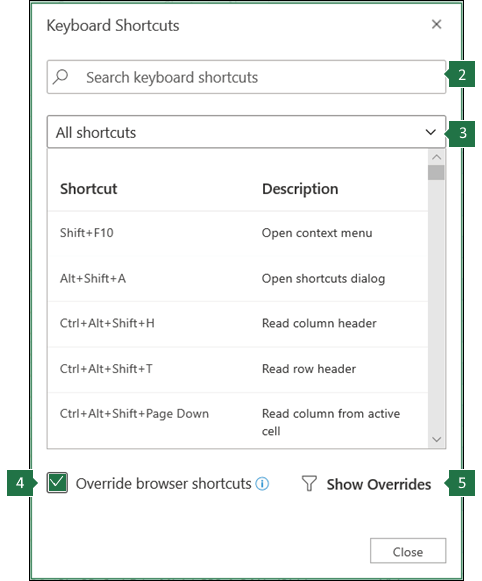
Control keyboard shortcuts in Excel for the web by overriding browser keyboard shortcuts

Quick tips for using keyboard shortcuts with Excel for the web

To find any command quickly, press Alt+Windows logo key, Q to jump to the Search or Tell Me text field. In Search or Tell Me, type a word or the name of a command you want (available only in Editing mode). Search or Tell Me searches for related options and provides a list. Use the Up and Down arrow keys to select a command, and then press Enter.

Depending on the version of Microsoft 365 you are using, the Search text field at the top of the app window might be called Tell Me instead. Both offer a largely similar experience, but some options and search results can vary.
To jump to a particular cell in a workbook, use the Go To option: press Ctrl+G, type the cell reference (such as B14), and then press Enter.
If you use a screen reader, go to Accessibility Shortcuts Menu (Alt+Shift+A).

Frequently used shortcuts

These are the most frequently used shortcuts for Excel for the web.

Tip: To quickly create a new worksheet in Excel for the web, open your browser, type Excel.new in the address bar, and then press Enter.

To do this	Press
Go to a specific cell.	Ctrl+G
Move down.	Page down or Down arrow key
Move up.	Page up or Up arrow key
Print a workbook.	Ctrl+P
Copy selection.	Ctrl+C
Paste selection.	Ctrl+V
Cut selection.	Ctrl+X
Undo action.	Ctrl+Z
Open workbook.	Ctrl+O
Close workbook.	Ctrl+W
Open the Save As dialog box.	Alt+F2
Use Find.	Ctrl+F or Shift+F3
Apply bold formatting.	Ctrl+B
Open the context menu.	Windows keyboards: Shift+F10 or Windows Menu key Other keyboards: Shift+F10
Jump to Search or Tell me.	Alt+Q
Repeat Find downward.	Shift+F4
Repeat Find upward.	Ctrl+Shift+F4
Insert a chart.	Alt+F1
Display the access keys (ribbon commands) on the classic ribbon when using Narrator.	Alt+Period (.)

Top of Page

Access keys: Shortcuts for using the ribbon

Excel for the web offers access keys, keyboard shortcuts to navigate the ribbon. If you’ve used access keys to save time on Excel for desktop computers, you’ll find access keys very similar in Excel for the web.

In Excel for the web, access keys all start with Alt+Windows logo key, then add a letter for the ribbon tab. For example, to go to the Review tab, press Alt+Windows logo key, R.

Note: To learn how to override the browser’s Alt-based ribbon shortcuts, go to Control keyboard shortcuts in Excel for the web by overriding browser keyboard shortcuts.

If you’re using Excel for the web on a Mac computer, press Control+Option to start.

To get to the ribbon, press Alt+Windows logo key, or press Ctrl+F6 until you reach the Home tab.
To move between tabs on the ribbon, press the Tab key.
To hide the ribbon so you have more room to work, press Ctrl+F1. To display the ribbon again, press Ctrl+F1.

Go to the access keys for the ribbon

To go directly to a tab on the ribbon, press one of the following access keys:

To do this	Press
Go to the Search or Tell Me field on the ribbon and type a search term.	Alt+Windows logo key, Q
Open the File menu.	Alt+Windows logo key, F
Open the Home tab and format text and numbers or use other tools such as Sort & Filter.	Alt+Windows logo key, H
Open the Insert tab and insert a function, table, chart, hyperlink, or threaded comment.	Alt+Windows logo key, N
Open the Data tab and refresh connections or use data tools.	Alt+Windows logo key, A
Open the Review tab and use the Accessibility Checker or work with threaded comments and notes.	Alt+Windows logo key, R
Open the View tab to choose a view, freeze rows or columns in your worksheet, or show gridlines and headers.	Alt+Windows logo key, W

Top of Page

Work in the ribbon tabs and menus

The shortcuts in this table can save time when you work with the ribbon tabs and ribbon menus.

To do this	Press
Select the active tab of the ribbon and activate the access keys.	Alt+Windows logo key. To move to a different tab, use an access key or the Tab key.
Move the focus to commands on the ribbon.	Enter, then the Tab key or Shift+Tab
Activate a selected button.	Spacebar or Enter
Open the list for a selected command.	Spacebar or Enter
Open the menu for a selected button.	Alt+Down arrow key
When a menu or submenu is open, move to the next command.	Esc

Top of Page

Keyboard shortcuts for editing cells

Tip: If a spreadsheet opens in the Viewing mode, editing commands won’t work. To switch to Editing mode, press Alt+Windows logo key, Z, M, E.

To do this	Press
Insert a row above the current row.	Alt+Windows logo key, H, I, R
Insert a column to the left of the current column.	Alt+Windows logo key, H, I, C
Cut selection.	Ctrl+X
Copy selection.	Ctrl+C
Paste selection.	Ctrl+V
Undo an action.	Ctrl+Z
Redo an action.	Ctrl+Y
Start a new line in the same cell.	Alt+Enter
Insert a hyperlink.	Ctrl+K
Insert a table.	Ctrl+L
Insert a function.	Shift+F3
Increase font size.	Ctrl+Shift+Right angle bracket (>)
Decrease font size.	Ctrl+Shift+Left angle bracket (<)
Apply a filter.	Alt+Windows logo key, A, T
Re-apply a filter.	Ctrl+Alt+L
Toggle AutoFilter on and off.	Ctrl+Shift+L

Top of Page

Keyboard shortcuts for entering data

To do this	Press
Complete cell entry and select the cell below.	Enter
Complete cell entry and select the cell above.	Shift+Enter
Complete cell entry and select the next cell in the row.	Tab key
Complete cell entry and select the previous cell in the row.	Shift+Tab
Cancel cell entry.	Esc

Top of Page

Keyboard shortcuts for editing data within a cell

To do this	Press
Edit the selected cell.	F2
Cycle through all the various combinations of absolute and relative references when a cell reference or range is selected in a formula.	F4
Clear the selected cell.	Delete
Clear the selected cell and start editing.	Backspace
Go to beginning of cell line.	Home
Go to end of cell line.	End
Select right by one character.	Shift+Right arrow key
Select to the beginning of cell data.	Shift+Home
Select to the end of cell data.	Shift+End
Select left by one character.	Shift+Left arrow key
Extend selection to the last nonblank cell in the same column or row as the active cell, or if the next cell is blank, to the next nonblank cell.	Ctrl+Shift+Right arrow key or Ctrl+Shift+Left arrow key
Insert the current date.	Ctrl+Semicolon (;)
Insert the current time.	Ctrl+Shift+Semicolon (;)
Copy a formula from the cell above.	Ctrl+Apostrophe (‘)
Copy the value from the cell above.	Ctrl+Shift+Apostrophe (‘)
Insert a formula argument.	Ctrl+Shift+A

Top of Page

Keyboard shortcuts for formatting cells

To do this	Press
Apply bold formatting.	Ctrl+B
Apply italic formatting.	Ctrl+I
Apply underline formatting.	Ctrl+U
Paste formatting.	Shift+Ctrl+V
Apply the outline border to the selected cells.	Ctrl+Shift+Ampersand (&)
Apply the number format.	Ctrl+Shift+1
Apply the time format.	Ctrl+Shift+2
Apply the date format.	Ctrl+Shift+3
Apply the currency format.	Ctrl+Shift+4
Apply the percentage format.	Ctrl+Shift+5
Apply the scientific format.	Ctrl+Shift+6
Apply outside border.	Ctrl+Shift+7
Open the Number Format dialog box.	Ctrl+1

Top of Page

Keyboard shortcuts for moving and scrolling within worksheets

To do this	Press
Move up one cell.	Up arrow key or Shift+Enter
Move down one cell.	Down arrow key or Enter
Move right one cell.	Right arrow key or Tab key
Go to the beginning of the row.	Home
Go to cell A1.	Ctrl+Home
Go to the last cell of the used range.	Ctrl+End
Move down one screen (28 rows).	Page down
Move up one screen (28 rows).	Page up
Move to the edge of the current data region.	Ctrl+Right arrow key or Ctrl+Left arrow key
Move between ribbon and workbook content.	Ctrl+F6
Move to a different ribbon tab.	Tab key Press Enter to go to the ribbon for the tab.
Insert a new sheet.	Shift+F11
Switch to the next sheet.	Alt+Ctrl+Page down
Switch to the next sheet (when in Microsoft Teams or a browser other than Chrome).	Ctrl+Page down
Switch to the previous sheet.	Alt+Ctrl+Page up
Switch to previous sheet (when in Microsoft Teams or a browser other than Chrome).	Ctrl+Page up

Top of Page

Keyboard shortcuts for working with objects

To do this	Press
Open menu or drill down.	Alt+Down arrow key
Close menu or drill up.	Alt+Up arrow key
Follow hyperlink.	Ctrl+Enter
Open a note for editing.	Shift+F2
Open and reply to a threaded comment.	Ctrl+Shift+F2
Rotate an object left.	Alt+Left arrow key
Rotate an object right.	Alt+Right arrow key

Top of Page

Keyboard shortcuts for working with cells, rows, columns, and objects

To do this	Press
Select a range of cells.	Shift+Arrow keys
Select an entire column.	Ctrl+Spacebar
Select an entire row.	Shift+Spacebar
Extend selection to the last nonblank cell in the same column or row as the active cell, or if the next cell is blank, to the next nonblank cell.	Ctrl+Shift+Right arrow key or Ctrl+Shift+Left arrow key
Add a non-adjacent cell or range to a selection.	Shift+F8
Insert cells, rows, or columns.	Ctrl+Plus sign (+)
Delete cells, rows, or columns.	Ctrl+Minus sign (-)
Hide rows.	Ctrl+9
Unhide rows.	Ctrl+Shift+9
Hide columns	Ctrl+0
Unhide columns	Ctrl+Shift+0

Top of Page

Keyboard shortcuts for moving within a selected range

To do this	Press
Move from top to bottom (or forward through the selection).	Enter
Move from bottom to top (or back through the selection).	Shift+Enter
Move forward through a row (or down through a single-column selection).	Tab key
Move back through a row (or up through a single-column selection).	Shift+Tab
Move to an active cell.	Shift+Backspace
Move to an active cell and keep the selection.	Ctrl+Backspace
Rotate the active cell through the corners of the selection.	Ctrl+Period (.)
Move to the next selected range.	Ctrl+Alt+Right arrow key
Move to the previous selected range.	Ctrl+Alt+Left arrow key
Extend selection to the last used cell in the sheet.	Ctrl+Shift+End
Extend selection to the first cell in the sheet.	Ctrl+Shift+Home

Top of Page

Keyboard shortcuts for calculating data

To do this	Press
Calculate workbook (refresh).	F9
Perform full calculation.	Ctrl+Shift+Alt+F9
Refresh external data.	Alt+F5
Refresh all external data.	Ctrl+Alt+F5
Apply Auto Sum.	Alt+Equal sign ( = )
Apply Flash Fill.	Ctrl+E

Top of Page

Accessibility Shortcuts Menu (Alt+Shift+A)

Access the common features quickly by using the following shortcuts:

To do this	Press
Cycle between landmark regions.	Ctrl+F6 or Ctrl+Shift+F6
Move within a landmark region.	Tab key or Shift+Tab
Go to the Search or Tell Me field to run any command.	Alt+Q
Display or hide Key Tips or access the ribbon.	Alt+Windows logo key
Edit the selected cell.	F2
Go to a specific cell.	Ctrl+G
Move to another worksheet in the workbook.	Ctrl+Alt+Page up or Ctrl+Alt+Page down
Open the context menu.	Shift+F10 or Windows Menu key
Read row header.	Ctrl+Alt+Shift+T
Read row until an active cell.	Ctrl+Alt+Shift+Home
Read row from an active cell.	Ctrl+Alt+Shift+End
Read column header.	Ctrl+Alt+Shift+H
Read column until an active cell.	Ctrl+Alt+Shift+Page up
Read column from an active cell.	Ctrl+Alt+Shift+Page down
Open a list of moving options within a dialog box.	Ctrl+Alt+Spacebar

Top of Page

Control keyboard shortcuts in Excel for the web by overriding browser keyboard shortcuts

Excel for the web works in a browser. Browsers have keyboard shortcuts, some of which conflict with shortcuts that work in Excel on the desktop. You can control these shortcuts, so they work the same in both versions of Excel by changing the Keyboard Shortcuts settings. Overriding browser shortcuts also enables you to open the Excel for the web Help by pressing F1.

Override browser shortcuts in Excel for the web dialog box.

In Excel for the web, select Help > Keyboard Shortcuts.
Search for any keyboard shortcut.
Choose the category of shortcuts to display in the list.
Select Override browser shortcuts.
Select Show Overrides to show shortcut overrides in the dialog box.
Select Close.

Top of Page

Technical support for customers with disabilities

Microsoft wants to provide the best possible experience for all our customers. If you have a disability or questions related to accessibility, please contact the Microsoft Disability Answer Desk for technical assistance. The Disability Answer Desk support team is trained in using many popular assistive technologies and can offer assistance in English, Spanish, French, and American Sign Language. Please go to the Microsoft Disability Answer Desk site to find out the contact details for your region.

If you are a government, commercial, or enterprise user, please contact the enterprise Disability Answer Desk.

Источник

For most marketers, trying to organize and analyze spreadsheets in Microsoft Excel can feel like walking into a brick wall repeatedly if you’e unfamiliar with Excel formulas. You’re manually replicating columns and scribbling down long-form math on a scrap of paper, all while thinking to yourself, «There has to be a better way to do this.»

Truth be told, there is — you just don’t know it yet.

Excel can be tricky that way. On the one hand, it’s an exceptionally powerful tool for reporting and analyzing marketing data. It can even help you visualize data with charts and pivot tables. On the other, without the proper training, it’s easy to feel like it’s working against you. For starters, there are more than a dozen critical formulas Excel can automatically run for you so you’re not combing through hundreds of cells with a calculator on your desk.

What are excel formulas?

Excel formulas help you identify relationships between values in the cells of your spreadsheet, perform mathematical calculations using those values, and return the resulting value in the cell of your choice. Formulas you can automatically perform include sum, subtraction, percentage, division, average, and even dates/times.

We’ll go over all of these, and many more, in this blog post.

How to Insert Formulas in Excel

You might wonder what the «Formulas» tab on the top navigation toolbar in Excel means. In more recent versions of Excel, this horizontal menu — shown below — allows you to find and insert Excel formulas into specific cells of your spreadsheet.

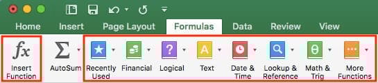
The more you use various formulas in Excel, the easier it’ll be to remember them and perform them manually. Nonetheless, the suite of icons above is a handy catalog of formulas you can browse and refer back to as you hone your spreadsheet skills.

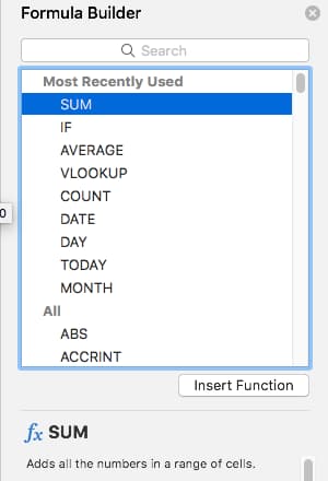
Excel formulas are also called «functions.» To insert one into your spreadsheet, highlight a cell in which you want to run a formula, then click the far-left icon, «Insert Function,» to browse popular formulas and what they do. That browsing window will look like this:

Want a more sorted browsing experience? Use any of the icons we’ve highlighted (inside the long red rectangle in the first screenshot above) to find formulas related to a variety of common subjects — such as finance, logic, and more. Once you’ve found the formula that suits your needs, click «Insert Function,» as shown in the window above.

Now, let’s do a deeper dive into some of the most crucial Excel formulas and how to perform each one in typical situations.

SUM
IF
Percentage
Subtraction
Multiplication
Division
DATE
Array
COUNT
AVERAGE
SUMIF
TRIM
LEFT, MID, and RIGHT
VLOOKUP
RANDOMIZE

To help you use Excel more effectively (and save a ton of time), we’ve compiled a list of essential formulas, keyboard shortcuts, and other small tricks and functions you should know.

NOTE: The following formulas apply to the latest version of Excel. If you’re using a slightly older version of Excel, the location of each feature mentioned below might be slightly different.

1. SUM

All Excel formulas begin with the equals sign, =, followed by a specific text tag denoting the formula you’d like Excel to perform.

The SUM formula in Excel is one of the most basic formulas you can enter into a spreadsheet, allowing you to find the sum (or total) of two or more values. To perform the SUM formula, enter the values you’d like to add together using the format, =SUM(value 1, value 2, etc).

The values you enter into the SUM formula can either be actual numbers or equal to the number in a specific cell of your spreadsheet.

To find the SUM of 30 and 80, for example, type the following formula into a cell of your spreadsheet: =SUM(30, 80). Press «Enter,» and the cell will produce the total of both numbers: 110.
To find the SUM of the values in cells B2 and B11, for example, type the following formula into a cell of your spreadsheet: =SUM(B2, B11). Press «Enter,» and the cell will produce the total of the numbers currently filled in cells B2 and B11. If there are no numbers in either cell, the formula will return 0.

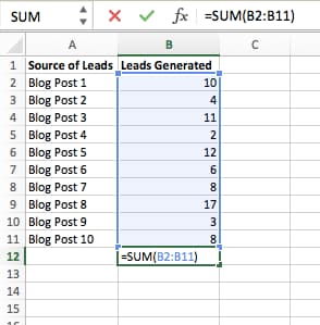
Keep in mind you can also find the total value of a list of numbers in Excel. To find the SUM of the values in cells B2 through B11, type the following formula into a cell of your spreadsheet: =SUM(B2:B11). Note the colon between both cells, rather than a comma. See how this might look in an Excel spreadsheet for a content marketer, below:

2. IF

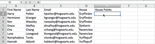
The IF formula in Excel is denoted =IF(logical_test, value_if_true, value_if_false). This allows you to enter a text value into the cell «if» something else in your spreadsheet is true or false. For example, =IF(D2=»Gryffindor»,»10″,»0″) would award 10 points to cell D2 if that cell contained the word «Gryffindor.»

There are times when we want to know how many times a value appears in our spreadsheets. But there are also those times when we want to find the cells that contain those values, and input specific data next to it.

We’ll go back to Sprung’s example for this one. If we want to award 10 points to everyone who belongs in the Gryffindor house, instead of manually typing in 10’s next to each Gryffindor student’s name, we’ll use the IF-THEN formula to say: If the student is in Gryffindor, then he or she should get ten points.

The formula: IF(logical_test, value_if_true, value_if_false)
- Logical_Test: The logical test is the «IF» part of the statement. In this case, the logic is D2=»Gryffindor.» Make sure your Logical_Test value is in quotation marks.
- Value_if_True: If the value is true — that is, if the student lives in Gryffindor — this value is the one that we want to be displayed. In this case, we want it to be the number 10, to indicate that the student was awarded the 10 points. Note: Only use quotation marks if you want the result to be text instead of a number.
- Value_if_False: If the value is false — and the student does not live in Gryffindor — we want the cell to show «0,» for 0 points.
Formula in below example: =IF(D2=»Gryffindor»,»10″,»0″)

3. Percentage

To perform the percentage formula in Excel, enter the cells you’re finding a percentage for in the format, =A1/B1. To convert the resulting decimal value to a percentage, highlight the cell, click the Home tab, and select «Percentage» from the numbers dropdown.

There isn’t an Excel «formula» for percentages per se, but Excel makes it easy to convert the value of any cell into a percentage so you’re not stuck calculating and reentering the numbers yourself.

The basic setting to convert a cell’s value into a percentage is under Excel’s Home tab. Select this tab, highlight the cell(s) you’d like to convert to a percentage, and click into the dropdown menu next to Conditional Formatting (this menu button might say «General» at first). Then, select «Percentage» from the list of options that appears. This will convert the value of each cell you’ve highlighted into a percentage. See this feature below.

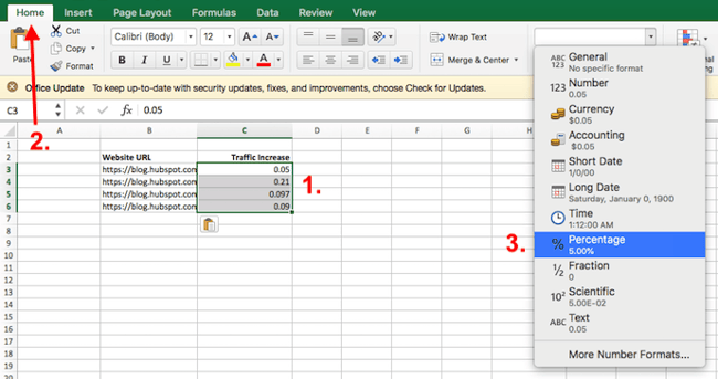
Keep in mind if you’re using other formulas, such as the division formula (denoted =A1/B1), to return new values, your values might show up as decimals by default. Simply highlight your cells before or after you perform this formula, and set these cells’ format to «Percentage» from the Home tab — as shown above.

4. Subtraction

To perform the subtraction formula in Excel, enter the cells you’re subtracting in the format, =SUM(A1, -B1). This will subtract a cell using the SUM formula by adding a negative sign before the cell you’re subtracting. For example, if A1 was 10 and B1 was 6, =SUM(A1, -B1) would perform 10 + -6, returning a value of 4.

Like percentages, subtracting doesn’t have its own formula in Excel either, but that doesn’t mean it can’t be done. You can subtract any values (or those values inside cells) two different ways.

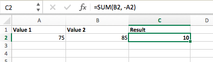
Using the =SUM formula. To subtract multiple values from one another, enter the cells you’d like to subtract in the format =SUM(A1, -B1), with a negative sign (denoted with a hyphen) before the cell whose value you’re subtracting. Press enter to return the difference between both cells included in the parentheses. See how this looks in the screenshot above.
Using the format, =A1-B1. To subtract multiple values from one another, simply type an equals sign followed by your first value or cell, a hyphen, and the value or cell you’re subtracting. Press Enter to return the difference between both values.

5. Multiplication

To perform the multiplication formula in Excel, enter the cells you’re multiplying in the format, =A1*B1. This formula uses an asterisk to multiply cell A1 by cell B1. For example, if A1 was 10 and B1 was 6, =A1*B1 would return a value of 60.

You might think multiplying values in Excel has its own formula or uses the «x» character to denote multiplication between multiple values. Actually, it’s as easy as an asterisk — *.

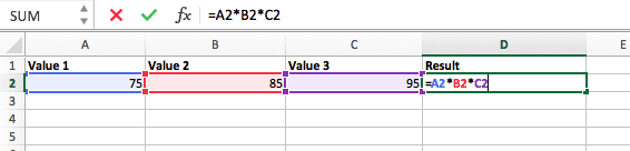
To multiply two or more values in an Excel spreadsheet, highlight an empty cell. Then, enter the values or cells you want to multiply together in the format, =A1*B1*C1 … etc. The asterisk will effectively multiply each value included in the formula.

Press Enter to return your desired product. See how this looks in the screenshot above.

6. Division

To perform the division formula in Excel, enter the cells you’re dividing in the format, =A1/B1. This formula uses a forward slash, «/,» to divide cell A1 by cell B1. For example, if A1 was 5 and B1 was 10, =A1/B1 would return a decimal value of 0.5.

Division in Excel is one of the simplest functions you can perform. To do so, highlight an empty cell, enter an equals sign, «=,» and follow it up with the two (or more) values you’d like to divide with a forward slash, «/,» in between. The result should be in the following format: =B2/A2, as shown in the screenshot below.

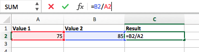
Hit Enter, and your desired quotient should appear in the cell you initially highlighted.

7. DATE

The Excel DATE formula is denoted =DATE(year, month, day). This formula will return a date that corresponds to the values entered in the parentheses — even values referred from other cells. For example, if A1 was 2018, B1 was 7, and C1 was 11, =DATE(A1,B1,C1) would return 7/11/2018.

Creating dates in the cells of an Excel spreadsheet can be a fickle task every now and then. Luckily, there’s a handy formula to make formatting your dates easy. There are two ways to use this formula:

Create dates from a series of cell values. To do this, highlight an empty cell, enter «=DATE,» and in parentheses, enter the cells whose values create your desired date — starting with the year, then the month number, then the day. The final format should look like this: =DATE(year, month, day). See how this looks in the screenshot below.
Automatically set today’s date. To do this, highlight an empty cell and enter the following string of text: =DATE(YEAR(TODAY()), MONTH(TODAY()), DAY(TODAY())). Pressing enter will return the current date you’re working in your Excel spreadsheet.

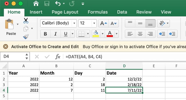
In either usage of Excel’s date formula, your returned date should be in the form of «mm/dd/yy» — unless your Excel program is formatted differently.

8. Array

An array formula in Excel surrounds a simple formula in brace characters using the format, {=(Start Value 1:End Value 1)*(Start Value 2:End Value 2)}. By pressing ctrl+shift+center, this will calculate and return value from multiple ranges, rather than just individual cells added to or multiplied by one another.

Calculating the sum, product, or quotient of individual cells is easy — just use the =SUM formula and enter the cells, values, or range of cells you want to perform that arithmetic on. But what about multiple ranges? How do you find the combined value of a large group of cells?

Numerical arrays are a useful way to perform more than one formula at the same time in a single cell so you can see one final sum, difference, product, or quotient. If you’re looking to find total sales revenue from several sold units, for example, the array formula in Excel is perfect for you. Here’s how you’d do it:

To start using the array formula, type «=SUM,» and in parentheses, enter the first of two (or three, or four) ranges of cells you’d like to multiply together. Here’s what your progress might look like: =SUM(C2:C5
Next, add an asterisk after the last cell of the first range you included in your formula. This stands for multiplication. Following this asterisk, enter your second range of cells. You’ll be multiplying this second range of cells by the first. Your progress in this formula should now look like this: =SUM(C2:C5*D2:D5)
Ready to press Enter? Not so fast … Because this formula is so complicated, Excel reserves a different keyboard command for arrays. Once you’ve closed the parentheses on your array formula, press Ctrl+Shift+Enter. This will recognize your formula as an array, wrapping your formula in brace characters and successfully returning your product of both ranges combined.

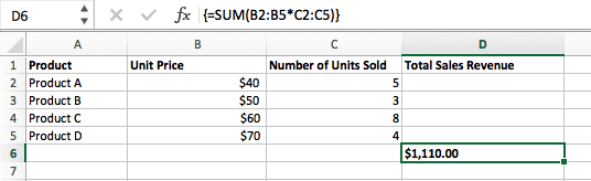
In revenue calculations, this can cut down on your time and effort significantly. See the final formula in the screenshot above.

9. COUNT

The COUNT formula in Excel is denoted =COUNT(Start Cell:End Cell). This formula will return a value that is equal to the number of entries found within your desired range of cells. For example, if there are eight cells with entered values between A1 and A10, =COUNT(A1:A10) will return a value of 8.

The COUNT formula in Excel is particularly useful for large spreadsheets, wherein you want to see how many cells contain actual entries. Don’t be fooled: This formula won’t do any math on the values of the cells themselves. This formula is simply to find out how many cells in a selected range are occupied with something.

Using the formula in bold above, you can easily run a count of active cells in your spreadsheet. The result will look a little something like this:

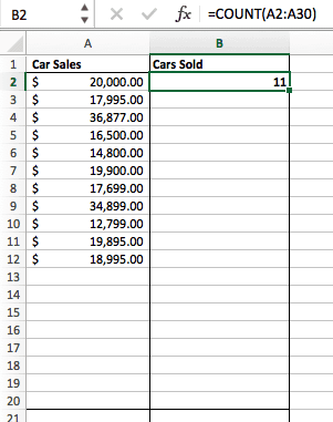
10. AVERAGE

To perform the average formula in Excel, enter the values, cells, or range of cells of which you’re calculating the average in the format, =AVERAGE(number1, number2, etc.) or =AVERAGE(Start Value:End Value). This will calculate the average of all the values or range of cells included in the parentheses.

Finding the average of a range of cells in Excel keeps you from having to find individual sums and then performing a separate division equation on your total. Using =AVERAGE as your initial text entry, you can let Excel do all the work for you.

For reference, the average of a group of numbers is equal to the sum of those numbers, divided by the number of items in that group.

11. SUMIF

The SUMIF formula in Excel is denoted =SUMIF(range, criteria, [sum range]). This will return the sum of the values within a desired range of cells that all meet one criterion. For example, =SUMIF(C3:C12,»>70,000″) would return the sum of values between cells C3 and C12 from only the cells that are greater than 70,000.

Let’s say you want to determine the profit you generated from a list of leads who are associated with specific area codes, or calculate the sum of certain employees’ salaries — but only if they fall above a particular amount. Doing that manually sounds a bit time-consuming, to say the least.

With the SUMIF function, it doesn’t have to be — you can easily add up the sum of cells that meet certain criteria, like in the salary example above.

The formula: =SUMIF(range, criteria, [sum_range])
- Range: The range that is being tested using your criteria.
- Criteria: The criteria that determine which cells in Criteria_range1 will be added together
- [Sum_range]: An optional range of cells you’re going to add up in addition to the first Range entered. This field may be omitted.

In the example below, we wanted to calculate the sum of the salaries that were greater than $70,000. The SUMIF function added up the dollar amounts that exceeded that number in the cells C3 through C12, with the formula =SUMIF(C3:C12,»>70,000″).

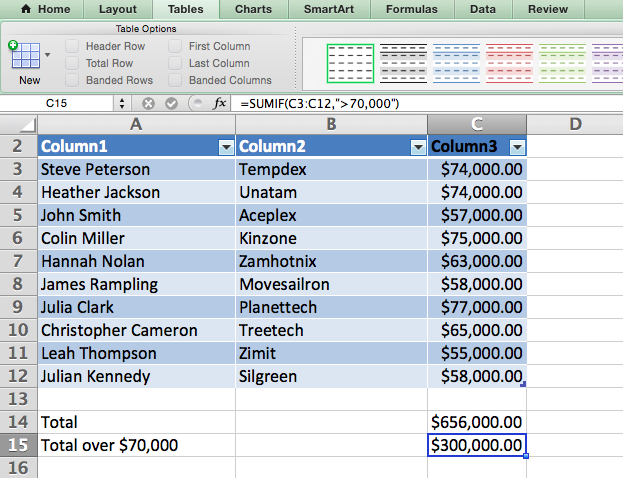
12. TRIM

The TRIM formula in Excel is denoted =TRIM(text). This formula will remove any spaces entered before and after the text entered in the cell. For example, if A2 includes the name » Steve Peterson» with unwanted spaces before the first name, =TRIM(A2) would return «Steve Peterson» with no spaces in a new cell.

Email and file sharing are wonderful tools in today’s workplace. That is, until one of your colleagues sends you a worksheet with some really funky spacing. Not only can those rogue spaces make it difficult to search for data, but they also affect the results when you try to add up columns of numbers.

Rather than painstakingly removing and adding spaces as needed, you can clean up any irregular spacing using the TRIM function, which is used to remove extra spaces from data (except for single spaces between words).

The formula: =TRIM(text).
- Text: The text or cell from which you want to remove spaces.

Here’s an example of how we used the TRIM function to remove extra spaces before a list of names. To do so, we entered =TRIM(«A2») into the Formula Bar, and replicated this for each name below it in a new column next to the column with unwanted spaces.

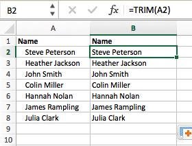
Below are some other Excel formulas you might find useful as your data management needs grow.

13. LEFT, MID, and RIGHT

Let’s say you have a line of text within a cell that you want to break down into a few different segments. Rather than manually retyping each piece of the code into its respective column, users can leverage a series of string functions to deconstruct the sequence as needed: LEFT, MID, or RIGHT.

LEFT

Purpose: Used to extract the first X numbers or characters in a cell.
The formula: =LEFT(text, number_of_characters)
- Text: The string that you wish to extract from.
- Number_of_characters: The number of characters that you wish to extract starting from the left-most character.

In the example below, we entered =LEFT(A2,4) into cell B2, and copied it into B3:B6. That allowed us to extract the first 4 characters of the code.

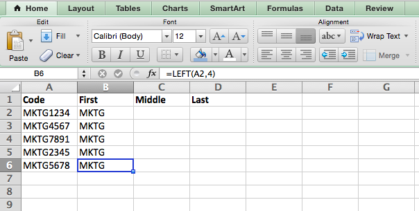
MID

Purpose: Used to extract characters or numbers in the middle based on position.
The formula: =MID(text, start_position, number_of_characters)
- Text: The string that you wish to extract from.
- Start_position: The position in the string that you want to begin extracting from. For example, the first position in the string is 1.
- Number_of_characters: The number of characters that you wish to extract.

In this example, we entered =MID(A2,5,2) into cell B2, and copied it into B3:B6. That allowed us to extract the two numbers starting in the fifth position of the code.

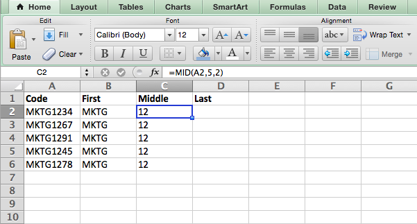
RIGHT

Purpose: Used to extract the last X numbers or characters in a cell.
The formula: =RIGHT(text, number_of_characters)
- Text: The string that you wish to extract from.
- Number_of_characters: The number of characters that you want to extract starting from the right-most character.

For the sake of this example, we entered =RIGHT(A2,2) into cell B2, and copied it into B3:B6. That allowed us to extract the last two numbers of the code.

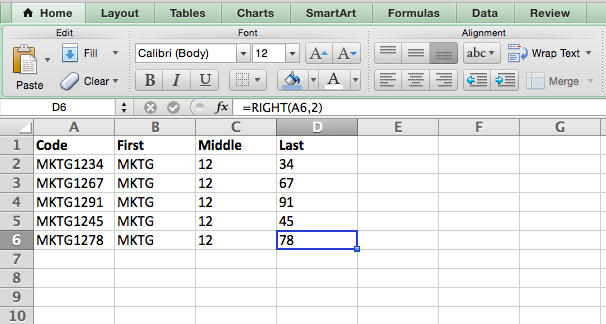
14. VLOOKUP

This one is an oldie, but a goodie — and it’s a bit more in depth than some of the other formulas we’ve listed here. But it’s especially helpful for those times when you have two sets of data on two different spreadsheets, and want to combine them into a single spreadsheet.

My colleague, Rachel Sprung — whose «How to Use Excel» tutorial is a must-read for anyone who wants to learn — uses a list of names, email addresses, and companies as an example. If you have a list of people’s names next to their email addresses in one spreadsheet, and a list of those same people’s email addresses next to their company names in the other, but you want the names, email addresses, and company names of those people to appear in one place — that’s where VLOOKUP comes in.

Note: When using this formula, you must be certain that at least one column appears identically in both spreadsheets. Scour your data sets to make sure the column of data you’re using to combine your information is exactly the same, including no extra spaces.

The formula: VLOOKUP(lookup value, table array, column number, [range lookup])
- Lookup Value: The identical value you have in both spreadsheets. Choose the first value in your first spreadsheet. In Sprung’s example that follows, this means the first email address on the list, or cell 2 (C2).
- Table Array: The range of columns on Sheet 2 you’re going to pull your data from, including the column of data identical to your lookup value (in our example, email addresses) in Sheet 1 as well as the column of data you’re trying to copy to Sheet 1. In our example, this is «Sheet2!A:B.» «A» means Column A in Sheet 2, which is the column in Sheet 2 where the data identical to our lookup value (email) in Sheet 1 is listed. The «B» means Column B, which contains the information that’s only available in Sheet 2 that you want to translate to Sheet 1.
- Column Number: The table array tells Excel where (which column) the new data you want to copy to Sheet 1 is located. In our example, this would be the «House» column, the second one in our table array, making it column number 2.
- Range Lookup: Use FALSE to ensure you pull in only exact value matches.
The formula with variables from Sprung’s example below: =VLOOKUP(C2,Sheet2!A:B,2,FALSE)

In this example, Sheet 1 and Sheet 2 contain lists describing different information about the same people, and the common thread between the two is their email addresses. Let’s say we want to combine both datasets so that all the house information from Sheet 2 translates over to Sheet 1. Here’s how that would work:

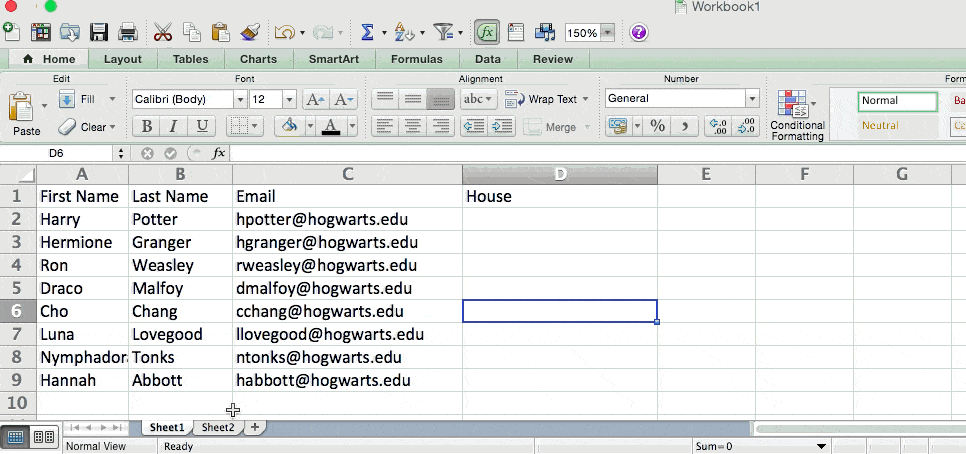
15. RANDOMIZE

There’s a great article that likens Excel’s RANDOMIZE formula to shuffling a deck of cards. The entire deck is a column, and each card — 52 in a deck — is a row. «To shuffle the deck,» writes Steve McDonnell, «you can compute a new column of data, populate each cell in the column with a random number, and sort the workbook based on the random number field.»

In marketing, you might use this feature when you want to assign a random number to a list of contacts — like if you wanted to experiment with a new email campaign and had to use blind criteria to select who would receive it. By assigning numbers to said contacts, you could apply the rule, “Any contact with a figure of 6 or above will be added to the new campaign.”

The formula: RAND()
- Start with a single column of contacts. Then, in the column adjacent to it, type “RAND()” — without the quotation marks — starting with the top contact’s row.
- RANDBETWEEN allows you to dictate the range of numbers that you want to be assigned. In the case of this example, I wanted to use one through 10.
- bottom: The lowest number in the range.
- top: The highest number in the range,For the example below: RANDBETWEEN(bottom,top)
- Formula in below example: =RANDBETWEEN(1,10)

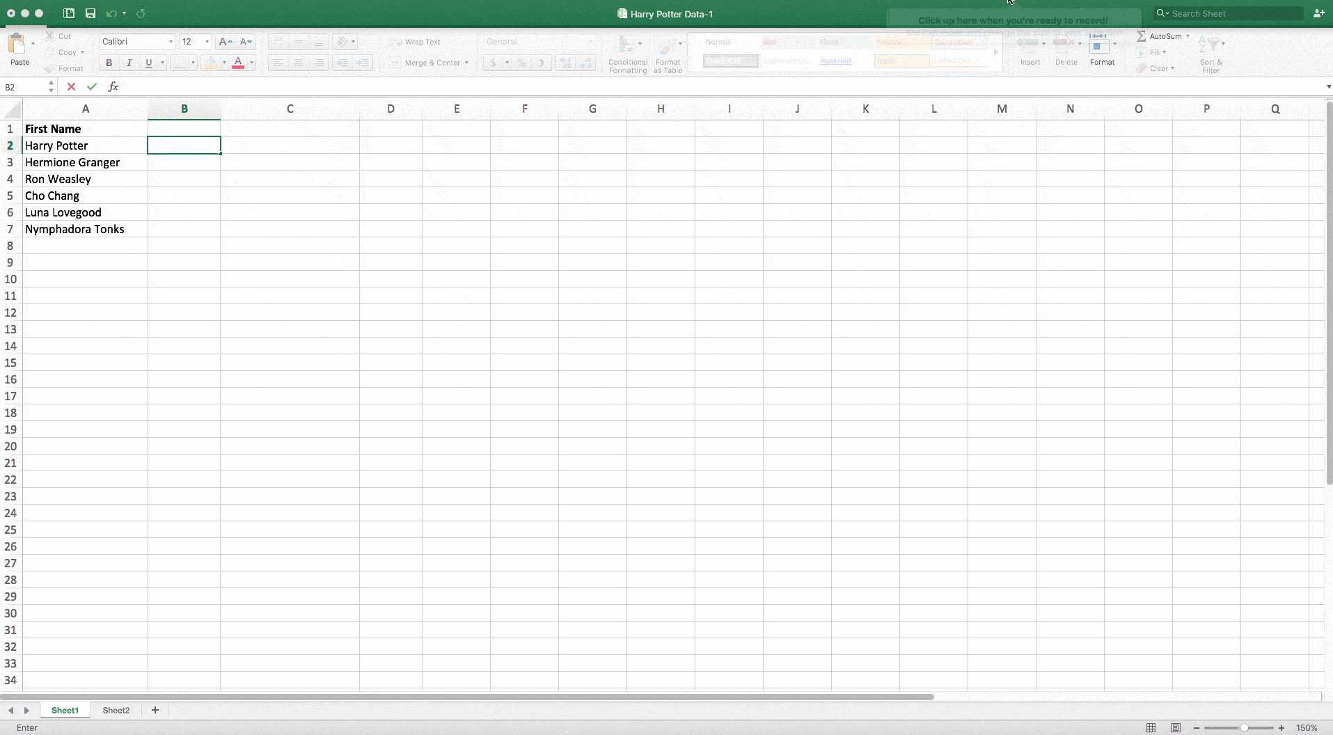
Helpful stuff, right? Now for the icing on the cake: Once you’ve mastered the Excel formula you need, you’ll want to replicate it for other cells without rewriting the formula. And luckily, there’s an Excel function for that, too. Check it out below.

Sometimes, you might want to run the same formula across an entire row or column of your spreadsheet. Let’s say, for example, you have a list of numbers in columns A and B of a spreadsheet and want to enter individual totals of each row into column C.

Obviously, it would be too tedious to adjust the values of the formula for each cell so you’re finding the total of each row’s respective numbers. Luckily, Excel allows you to automatically complete the column; all you have to do is enter the formula in the first row. Check out the following steps:

Type your formula into an empty cell and press «Enter» to run the formula.
Hover your cursor over the bottom-right corner of the cell containing the formula. You’ll see a small, bold «+» symbol appear.
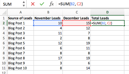
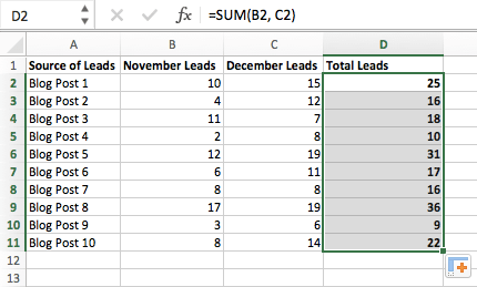While you can double-click this symbol to automatically fill the entire column with your formula, you can also click and drag your cursor down manually to fill only a specific length of the column.Once you’ve reached the last cell in the column you’d like to enter your formula, release your mouse to copy the formula. Then, simply check each new value to ensure it corresponds to the correct cells.

Excel Keyboard Shortcuts

1. Quickly select rows, columns, or the whole spreadsheet.

Perhaps you’re crunched for time. I mean, who isn’t? No time, no problem. You can select your entire spreadsheet in just one click. All you have to do is simply click the tab in the top-left corner of your sheet to highlight everything all at once.

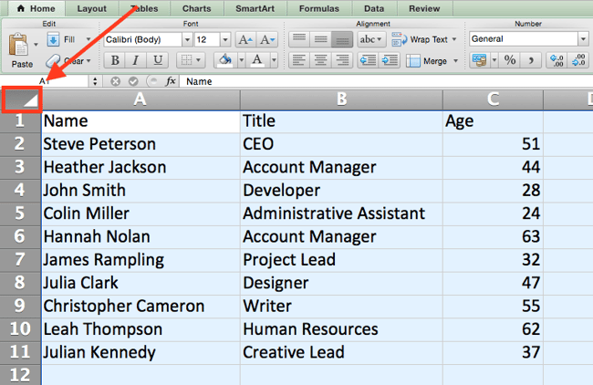
Just want to select everything in a particular column or row? That’s just as easy with these shortcuts:

For Mac:

Select Column = Command + Shift + Down/Up
Select Row = Command + Shift + Right/Left

For PC:

Select Column = Control + Shift + Down/Up
Select Row = Control + Shift + Right/Left

This shortcut is especially helpful when you’re working with larger data sets, but only need to select a specific piece of it.

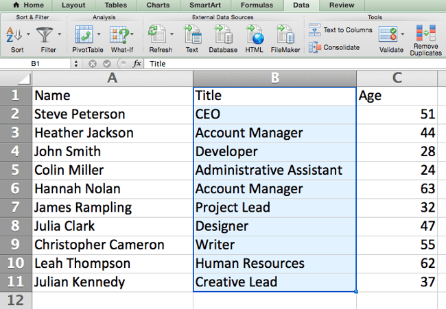
2. Quickly open, close, or create a workbook.

Need to open, close, or create a workbook on the fly? The following keyboard shortcuts will enable you to complete any of the above actions in less than a minute’s time.

For Mac:

Open = Command + O
Close = Command + W
Create New = Command + N

For PC:

Open = Control + O
Close = Control + F4
Create New = Control + N

3. Format numbers into currency.

Have raw data that you want to turn into currency? Whether it be salary figures, marketing budgets, or ticket sales for an event, the solution is simple. Just highlight the cells you wish to reformat, and select Control + Shift + $.

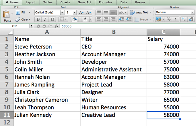
The numbers will automatically translate into dollar amounts — complete with dollar signs, commas, and decimal points.

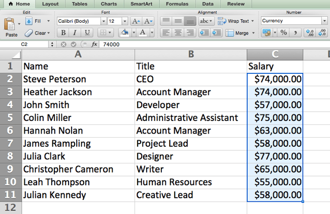
Note: This shortcut also works with percentages. If you want to label a column of numerical values as «percent» figures, replace «$» with «%».

4. Insert current date and time into a cell.

Whether you’re logging social media posts, or keeping track of tasks you’re checking off your to-do list, you might want to add a date and time stamp to your worksheet. Start by selecting the cell to which you want to add this information.

Then, depending on what you want to insert, do one of the following:

Insert current date = Control + ; (semi-colon)
Insert current time = Control + Shift + ; (semi-colon)
Insert current date and time = Control + ; (semi-colon), SPACE, and then Control + Shift + ; (semi-colon).

Other Excel Tricks

1. Customize the color of your tabs.

If you’ve got a ton of different sheets in one workbook — which happens to the best of us — make it easier to identify where you need to go by color-coding the tabs. For example, you might label last month’s marketing reports with red, and this month’s with orange.

Simply right click a tab and select «Tab Color.» A popup will appear that allows you to choose a color from an existing theme, or customize one to meet your needs.

2. Add a comment to a cell.

When you want to make a note or add a comment to a specific cell within a worksheet, simply right-click the cell you want to comment on, then click Insert Comment. Type your comment into the text box, and click outside the comment box to save it.

Cells that contain comments display a small, red triangle in the corner. To view the comment, hover over it.

3. Copy and duplicate formatting.

If you’ve ever spent some time formatting a sheet to your liking, you probably agree that it’s not exactly the most enjoyable activity. In fact, it’s pretty tedious.

For that reason, it’s likely that you don’t want to repeat the process next time — nor do you have to. Thanks to Excel’s Format Painter, you can easily copy the formatting from one area of a worksheet to another.

Select what you’d like to replicate, then select the Format Painter option — the paintbrush icon — from the dashboard. The pointer will then display a paintbrush, prompting you to select the cell, text, or entire worksheet to which you want to apply that formatting, as shown below:

4. Identify duplicate values.

In many instances, duplicate values — like duplicate content when managing SEO — can be troublesome if gone uncorrected. In some cases, though, you simply need to be aware of it.

Whatever the situation may be, it’s easy to surface any existing duplicate values within your worksheet in just a few quick steps. To do so, click into the Conditional Formatting option, and select Highlight Cell Rules > Duplicate Values

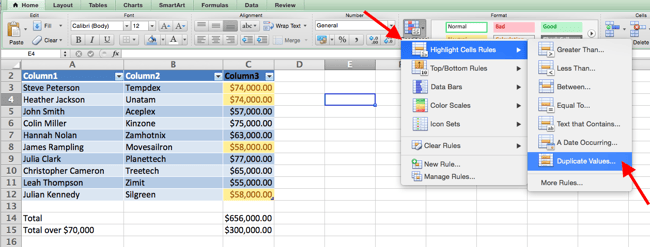
Using the popup, create the desired formatting rule to specify which type of duplicate content you wish to bring forward.

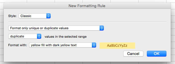
In the example above, we were looking to identify any duplicate salaries within the selected range, and formatted the duplicate cells in yellow.

5. Correcting a ### value error.

If the column isn’t wide enough to display the contents in the cell, Excel may display ### instead. To fix and make the column wider, simply double-click the top right corner of the column header and drag it to the size you want.

Alternatively, you could also shrink the contents to fit the cell by going:

Home > Alignment and then check the Shrink to fit box in the Format Cells dialog box.

Excel Shortcuts Save You Time

In marketing, the use of Excel is pretty inevitable — but with these tricks, it doesn’t have to be so daunting. As they say, practice makes perfect. The more you use these formulas, shortcuts, and tricks, the more they’ll become second nature.

Editor’s note: This post was originally published in January 2019 and has been updated for comprehensiveness.

Источник

Worksheets and Workbooks

View

Row and Column Selection

Ribbon Control

Pivot Tables

Operating within a Cell

Navigating and Selecting Cells

Help and Menus

Group Selection

General Excel

General Cell Control

Formulas and Functions

By adding formulas and functions to your Excel sheet, you instantly gain access to a wealth of information regarding your data and can conduct complex calculations with ease. These shortcuts can help Excel beginners and even advanced users begin building formulas and functions, as well as receive help where necessary.

Formatting Text and Numbers

Dialog Boxes

Borders

Advanced Selection

Adding Content to Cells

Get more Reference tips and tricks

Subscribe to our email updates and get Reference tips direct to your inbox.

Источник

What are Excel Shortcuts?

An Excel shortcut is a technique of performing a manual task in a quicker way. The shortcuts help speed up the work, which saves time for the secondary tasks of the job. Since Excel is used by almost everybody in some form or the other, it is essential to be aware of the shortcuts.

For example, the excel shortcut “Ctrl+O” opens an already existing workbook. The shortcut “Ctrl+W” closes the currently active workbook.

The purpose of using an excel shortcut is to save the worksheet creator from extra clicks. This improves the productivity at the workplace.

At times, the same task is repeated in Excel on a daily basis. Since such tasks may not have a shortcut, the solution is to create it by recording a macro.

What are Excel Shortcuts?
Top 20 Keyboard Shortcuts in Excel
- #1–Paste as Values With “Paste Special”
- #2–Sum Numbers With AutoSum
- #3–Fill the Subsequent Cell With the Fill Down
- #4–Select the Entire Row or Column
- #5–Insert and Delete Row or Column
- #6–Insert and Edit Comment
- #7–Move Between Sheets
- #8–Add Filters
- #9–Freeze Rows and Columns
- #10–Open “Format Cells” Dialog Box
- #11–Adjust Column Width
- #12–Repeat the Last Task
- #13–Insert Line Breaks in a Cell
- #14–Move Between Different Workbooks
- #15–Spell-Check
- #16–Move Between Worksheet and Excel VBA Editor
- #17–Select a Cell Range
- #18–Select the Last Non-Blank Cell of a Row or Column
- #19–Delete the Active Sheet
- #20–Insert a New Sheet
- Frequently Asked Questions
- Recommended Articles

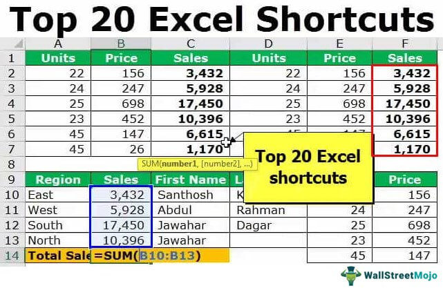
This article discusses the important excel shortcuts which have been consolidated keeping in mind the day-to-day needs of the user. The explanation of each technique is followed by a relevant example.

It is not possible to memorize every excel shortcut. However, a regular usage does allow gradual learning. To develop expertise in Excel, it is imperative to go beyond the basic cut (Ctrl+X), copy (Ctrl+C), and paste (Ctrl+V) shortcuts.

#1–Paste as Values With “Paste Special”

If a formula cell is copied and pasted, its formula is pasted and not the value of the cell. With “paste specialPaste special in Excel allows you to paste partial aspects of the data copied. There are several ways to paste special in Excel, including right-clicking on the target cell and selecting paste special, or using a shortcut such as CTRL+ALT+V or ALT+E+S.read more,” it is possible to paste the value of the formula cell at the desired location.

The excel shortcut “Alt+E+S+V” (press one by one) opens the “paste special” window and selects “values” under “paste.”

Note: Prior to pressing the excel shortcut, the formula cell must be copied and the desired output cell (where output is required) should be selected.

Example

The succeeding table shows the prices (in $ in column B) at which some units (column A) of a product are sold. We want to calculate the sales figures and, instead of formulas, paste the final values in column C.

Use the shortcut of the “paste special” property.

The steps to calculate sales and apply the “paste special” shortcut are listed as follows:

Step 1: In cell C2, enter the following formula.

“=B2*A2”

The cell C2 is dependent on the cells A2 and B2.

Copy-paste or drag the formula to the remaining cells. The formulas are applied to the entire range (C2:C6).

Step 2: Copy the formula cell C2. Press the keys “ALT+E+S+V” one by one. The “paste special” window opens. “Values” is automatically selected under “paste.” Click “Ok.”

Step 3: The number 3,432 is pasted in cell C2 as a value and not as a formula.

#2–Sum Numbers With AutoSum

Often, there is a need to sum a set of numbers. To do this, we usually apply the SUM functionThe SUM function in excel adds the numerical values in a range of cells. Being categorized under the Math and Trigonometry function, it is entered by typing “=SUM” followed by the values to be summed. The values supplied to the function can be numbers, cell references or ranges.read more. An alternative method is to use the excel shortcut key.

The shortcut “Alt+=” (press together) sums numbers.

Example #2

The following table shows the region-wise sales of an organization. We want to sum all the sales figures to find the total sales. Use the shortcut of AutoSum.

Step 1: Select cell B6. Press the excel shortcut keys “Alt+=” together.

Step 2: The SUM formula automatically appears in cell B6, as shown in the following image.

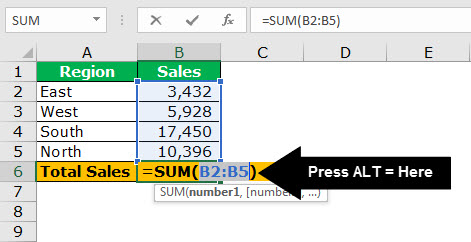
#3–Fill the Subsequent Cell With the Fill Down

The fill downWhen you want to fill down or copy any data or formulas to the cells down below, you can use Excel fill down. While copying the data and selecting the cells, the keyboard shortcut is CTRL + D.read more property fills the present (subsequent) cell with the value or formula of the immediately preceding cell. This feature is often used while entering data in Excel.

The excel shortcut “Ctrl+D” (press together) fills the immediately following cell with the data or formula of the preceding cell.

If a range of cells is selected, the content of the topmost cell is filled in the cells below. If the subsequent cell already contains a value, pressing “Ctrl+D” overwrites it.

Note 1: If the preceding cell contains a value, the fill down feature copies the same to the immediately following cell. However, if the preceding cell contains a formula, the same is copied.

Note 2: While copying a formula, the cell references may or may not change depending on the kind of references used (relative or absolute).

Note 3: The shortcut “Ctrl+D” works only for columns and not for rows. For rows, use the shortcut “Ctrl+R” (press together), which fills cells to the right.

Example

The left side of the following image shows the first and the last names in columns A and B respectively. We want to copy the first name of row 4 in row 5 with the help of the fill down excel shortcut.

Step 1: Select cell A5. Press the keys “Ctrl+D” together.

Step 2: The name “Jawahar” is copied to cell A5, as shown by the right side of the following image.

Example

The left side of the following image shows the sales (column G) calculated by multiplying the price (column F) with the number of units (column E).

We want to calculate the sales (units=45 and price=26) for the entry in row 7. Use the fill down shortcut.

Step 1: Enter 26 as the price in cell F7. Select cell G7 and press the keys “Ctrl+D.”

Step 2: The formula of the preceding cell (G6) is copied to cell G7, as shown by the right side of the following image.

#4–Select the Entire Row or Column

Often, there is a need to select the entire row or column in Excel.

The excel shortcut “Shift+space” (press together) selects the entire row.

The shortcut “Ctrl+space” (press together) selects the entire column.

Example

The following image shows a blank worksheet. With the help of the shortcut, we want to:

a) Select row 4 in the given worksheet

b) Select column B in the given worksheet

a) Step 1: Select any cell in row 4. Press the excel shortcut keys “Shift+space” together.

Step 2: The entire row 4 is selected, as shown in the following image.

b) Step 1: Select any cell in column B. Press the shortcut keys “Ctrl+space” together.

Step 2: The entire column B is selected, as shown in the following image.

#5–Insert and Delete Row or Column

At times, we may need to insert or delete a rowTo delete a row or a set of rows from a spreadsheet, first select the row or rows you want to delete, then hit CTRL – (minus sign) as a shortcut key.read more or column.

The excel shortcut “Ctrl+Shift+plus sign (+)” inserts a new row or column. The keys must be pressed together.

Prior to pressing this shortcut, select the entire row or column preceding which the insertion has to be made. For this, click the row or column label appearing at the leftmost side or on top.

The excel shortcut “Ctrl+minus sign (-)” deletes an existing row or column. The keys must be pressed together.

Prior to pressing this shortcut, select the entire row or column which has to be deleted.

Note: If the preceding shortcuts (insert or delete) are pressed by selecting a cell rather than the entire row or column, the “insert” or “delete” dialog box opens.

Example

The following image shows the number of units (column E), prices (column F), and sales (column G). With the help of the shortcut, we want to:

a) Insert a row preceding row 4

b) Delete the newly inserted row 4.

a) Step 1: Select the entire row 4 by clicking the label “4” at the leftmost side.

Step 2: Press the keys “Ctrl+Shift+plus sign (+)” together.

Step 3: A row preceding row 4 is inserted, as shown in the following image.

b) Step 1: Click the row label to select the entire row 4.

Step 2: Press the keys “Ctrl+minus sign(-)” together.

Step 3: The newly inserted row (inserted in step 3 of the preceding solution) is deleted. The same is shown in the following image.

#6–Insert and Edit Comment

In Excel, we may need to enter comments for a specific cell. This saves the information related to that cell and allows returning to the same, if required.

The excel shortcut “right-click+M” (press one by one) inserts a new comment on a cell.

The right-click button (menu or the context key) on the keyboard opens the context menu for the selected item. The menu key is located at the bottom, to the right side of the spacebar. It is placed between the right side “Alt” and the right side “Ctrl” key.

Prior to pressing the shortcut, it is important to select the cell in which a comment is to be inserted.

Note: Alternatively, press “Shift+F10” (press together) to open the context menu. Thereafter, press “M” to insert a comment.

The excel shortcut “Shift+F2” (press together) helps edit a comment.

Prior to pressing the shortcut, select the cell containing the comment to be edited.

Example

Working on the data of example #6, we want to:

a) Insert a comment on cell C2

b) Edit the comment of cell C2

Use the shortcut of inserting and editing comments.

a) Step 1: Select the cell C2. Press the menu key followed by “M.”

Step 2: A comment is inserted on cell C2, as shown in the following image.

b) Step 1: Select the cell C2. Press the keys “Shift+F2” together.

Step 2: The cursor appears inside the comment. The comment can now be edited, as shown in the following image.

#7–Move Between Sheets

While working in Excel, different sheets are required to be dealt with at one time. Moreover, it is tedious to click the sheet labels at the bottom of the workbook. The shortcuts help in quickly navigating through the sheets.

The excel shortcut “Ctrl+page down” (press together) helps move from the currently active sheet to the next sheet.

The excel shortcut “Ctrl+page up” (press together) helps move from the currently active sheet to the preceding sheet.

For example, the sheet names are “sheet 1,” “sheet 2,” and “sheet 3” and the current active sheet is “sheet 2.” To go to “sheet 3,” press “Ctrl+page down.” Press “Ctrl+page up” to move to “sheet 1.”

Example

The following image shows the different data sheets of a workbook. With the help of the excel shortcut, we want to:

a) Move from the “insert comment” sheet to the “freeze rows & column” sheet

b) Move from the “freeze rows & column” sheet back to the “insert comment” sheet

a) Step 1: Press the keys “Ctrl+page down” together.

Step 2: There is a movement from “insert comment” to “freeze rows & column” sheet. The latter sheet is now the currently active sheet.

b) Step 1: Press the keys “Ctrl+page up” together.

Step 2: There is a movement from “freeze rows & column” to “insert comment” sheet. The currently active sheet now is the “insert comment” sheet.

#8–Add Filters

To add or remove filters from a dataset, select “filter” from the Data tab or the Home tab (“sort and filter” drop-down) of the Excel ribbonThe ribbon is an element of the UI (User Interface) which is seen as a strip that consists of buttons or tabs; it is available at the top of the excel sheet. This option was first introduced in the Microsoft Excel 2007.read more. However, this method is manual and takes time.

The excel shortcuts “Ctrl+Shift+L” (press together) or “Alt+D+F+F” (press one by one) add and remove filters.

Example

Working on the data of example #6, we want to insert filters on columns A, B, and C. Thereafter, remove these filters. Use the shortcut keys.

Step 1: Select cell A1. Press the keys “Ctrl+Shift+L” together. Alternatively, press the keys “Alt+D+F+F” one by one.

Step 2: The filters are added to columns A, B, and C.

Step 3: Press the preceding shortcuts (pressed in step 1) again. The filters are removed.

The insertion and removal of filters are shown in the following image.

#9–Freeze Rows and Columns

While working in Excel, there may be a need to freeze the first row and the first column. Once frozen, the given row and column do not move while scrolling through the remaining data.

The excel shortcut “Alt+W+F+F” (press one by one) freezes the rows and/or columns based on the current selection of cell.

To freeze the first row and the first column, select cell B2.

Note: The given shortcut freezes the rows preceding the currently selected cell. At the same time, the columns to the left of the currently selected cell are also frozen.

Example

The following image shows the username and the passwords in columns A and B respectively. We want to freeze the first row and the first column with the help of the shortcut keys.

Step 1: Select cell B2. Press the shortcut “Alt+W+F+F” one by one.

Step 2: The first row and the first column are frozen, as shown in the following image.

#10–Open “Format Cells” Dialog Box

The “format cells” dialog box helps format a cell or a cell range of Excel. To open this box manually, select a cell and right-click the same. Thereafter, choose the “format cells” option from the context menu.

The shortcut “Ctrl+1” (press together) opens the “format cells” dialog box.

Example

We want to open the “format cells” dialog box in an Excel worksheet with the help of the shortcut.

Step 1: In the worksheet, press “Ctrl+1” together.

Step 2: The “format cells” dialog box appears, as shown in the following image.

#11–Adjust Column Width

To adjust the width of a columnA user can set the width of a column in an excel worksheet between 0 and 255, where one character width equals one unit. The column width for a new excel sheet is 8.43 characters, which is equal to 64 pixels.read more, one needs to double-click the column edge. This task can also be done with the help of a shortcut.

The excel shortcut “Alt+O+C+A” (press one by one) adjusts the width of the selected column.

Example

The left side of the following image shows the usernames in column A. Since the width of this column has not been adjusted, some entries are exceeding its right-side border.

We want to adjust the width of column A with the help of the shortcut keys.

Step 1: Select the column (column A) whose width has to be adjusted.

Step 2: Press the shortcut keys “Alt+O+C+A” one by one.

Step 3: The column width is adjusted, as shown by the right side of the following image. Hence, all entries fit in column A.

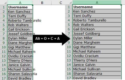
#12–Repeat the Last Task

In Excel, one may need to repeat the last task or action performed. This task can be formatting, inserting a new row or column, deleting an existing row or column, and so on.

The shortcut “F4” repeats the last task, if possible.

#13–Insert Line Breaks in a Cell

While typing in a cell, there may be a need to insert a line break. The line break helps add spacing between the sentences of a cell. Once a line break is added, the user can begin a new sentence in the same cell.

The excel shortcut “Alt+Enter” (press together) inserts a line break within a cell.

Example

The following image shows a question in cell A1. We want to insert a line break in order to type a new sentence within the same cell A1. Use the shortcut for the same.

Step 1: Double-click the cell (cell A1) within which a line break is to be inserted.

Step 2: Click at the place (after the two question marks) where the line break is to be inserted.

Step 3: Press the keys “Alt+Enter” together. The line break appears, as shown in the following image. Hence, after the spacing has been inserted, the user can begin a new sentence in cell A1.

#14–Move Between Different Workbooks

To switch between various windows, the shortcut “Alt+tab” is used. However, often while working, one needs to move from one workbook to another.

The excel shortcut “Ctrl+tab” (press together) helps switch between the open workbooks.

#15–Spell-Check

Prior to submitting an Excel worksheet to seniors at the workplace, it is essential to do a quick spell-check. This lets the user know the mistakes and the corrections that should be followed presently and in the future.

The excel shortcut “F7” helps perform a spell-check of the currently active worksheet.

Example

The following image shows the usernames in column A. We want to run a spell-check on this worksheet with the help of the shortcut.

Step 1: Press the shortcut “F7.”

Step 2: The “spelling” dialog box appears, as shown in the following image. Hence, the spellings of column A can be corrected by matching them against the suggestions.

#16–Move Between Worksheet and Excel VBA Editor

While working with macros, one needs to move between the VBA editorThe Visual Basic for Applications Editor is a scripting interface. These scripts are primarily responsible for the creation and execution of macros in Microsoft software.read more and the Excel worksheet.

The excel shortcut “Alt+F11” helps switch between the VBA editor and the worksheet.

#17–Select a Cell Range

Selecting the cell ranges of Excel can be a time-consuming task, if done manually.

The excel shortcut “Ctrl+Shift+arrow keys” selects the cell ranges of Excel.

Note: The selection of cells, in the same row or column as the currently active cell, is carried out till the last non-blank cell. However, if the following cell (in the same row or column as the currently active cell) is blank, the selection is carried out till the next non-blank cell.

Example

The following image shows the usernames, passwords, designations, titles, and first names in columns A, B, C, D, and E respectively. We want to select the range A1:E100 with the help of the shortcut.

Step 1: Select cell A1. Press the keys “Ctrl+Shift+right arrow” to select till cell E1.

Step 2: Press the keys “Ctrl+Shift+down arrow” to select till cell E100.

Step 3: The range A1:E100 is selected, as shown in the following image.

#18–Select the Last Non-Blank Cell of a Row or Column

Beginning from cell A1, one may need to go to the last cell of column A. This requires manual scrolling, which is a difficult task, particularly when working with large datasets.

The excel shortcut “Ctrl+down arrow” (press together) helps the user go to the last non-blank cell of the current column (column of the active cell).

The excel shortcut “Ctrl+right arrow” (press together) helps the user go to the last non-blank cell of the current row (row of the active cell).

Note: In case the cell immediately following the active cell is blank, the next non-blank cell is selected.

Example

The following table shows the usernames and passwords in columns A and B respectively. We want to go to the cell A100, which is the last non-blank cell of column A. Use the shortcut keys.

Step 1: Select cell A1. Press the keys “Ctrl+down arrow” together.

Step 2: The last cell (A100) of the dataset is selected, as shown in the following image.

#19–Delete the Active Sheet

To delete a sheet manually, one can right-click the sheet name and select “delete.” Alternatively, the shortcut helps do the same quickly.

The excel shortcut “Alt+E+L” (press one by one) deletes the currently active sheet.

Once the given shortcut is pressed, a message appears stating that the data of the worksheet will be permanently deleted. Click “delete” to delete the sheet, otherwise press “cancel.”

#20–Insert a New Sheet

Often, new sheets are required to be added to the workbook. It is possible to insert a new sheet with a single click.

The excel shortcut “Shift+F11” (press together) inserts a new sheet in the current workbook.

The excel shortcut “F11” inserts a chart sheet in which a chart can be created by selecting a data range.

Frequently Asked Questions

1. What are Excel shortcuts and how to use them?

An Excel shortcut helps perform a manual task in a faster way. With the application of shortcuts, the user saves time and improves the productivity. This saved time can be used for focusing on other projects of a job role.

The list of Excel shortcuts is a large one. There are shortcuts for entering, formatting, deleting, and selecting data. So, it is not possible to learn all the shortcuts. However, knowing the regularly used ones is essential.

To use an Excel shortcut, press the particular keys on the keyboard. But, prior to using it, one must know whether to press the keys simultaneously or one by one. This is because each shortcut works in a specific way.

2. What are the basic Excel shortcuts and how to learn them?

The basic Excel shortcuts are listed as follows:

Ctrl+S: It saves a workbook.
Ctrl+A: It selects the entire worksheet.
Ctrl+B: It makes the content of the selected cells bold.
Ctrl+C: It copies the selected cell.
Ctrl+I: It italicizes the content of the selected cell.
Ctrl+P: It opens the “print” dialog box.
Ctrl+X: It cuts the content of the selected cell.
Ctrl+V: It pastes in the currently selected cell.
Ctrl+Z: It undoes the last action.

Excel shortcuts can be learned with regular usage and practice. The more you practice working on Excel, the more habitual you will become. In this way, you can learn gradually.

Note: The keys of all the preceding shortcuts should be pressed simultaneously.

3. How to work with Excel formulas by way of shortcuts?

The “tab” key is an important shortcut used for auto-completing the name of the function. For instance, to enter the CONCATENATE function in a cell, type “=CON” and press the “tab” key. The CONCATENATE function is automatically selected.

With the “F4” key, one can toggle between the relative, absolute, and mixed references. Double-click the formula cell and press “F4” to change the type of reference.

Likewise, different keyboard keys have different functions. By applying shortcuts to Excel formulas, one can simplify working with calculations.

Here is the complete list of excel keyboard shortcuts.

Shortcuts for Selection
Shortcuts for Editing
Shortcuts for Navigation
Shortcuts for Formatting
Shortcuts for Formulas
Shortcuts for Excel Options
Shortcuts for Auto Complete
Shortcuts for Everything Else

Note: I have *ed some of the most important shortcuts. These are very useful and extremely time saving ones. You may want to remember a few to boost your productivity.

Select the whole column

Selection

CTRL + SPACE

Select the whole row

Selection

SHIFT + SPACE

Select table

Selection

SHIFT + CTRL + SPACE bar

Save

Selection

CTRL + s

Select visible cells only

Selection

ALT + ;

Select entire region

Selection

CTRL + A

Select range from start cell to far left

Selection

SHIFT + Home

Select range from start cell to end in direction of arrow

Selection

SHIFT + End + arrow

Select a continuous range of data (e.g. pivot), no matter where your cursor is.

Selection

CTRL + *

Select blank cells

Selection

F5 + ALT + S + K + ENTER

Select all cells with comments

Selection

CTRL + SHIFT + O

Select all cells that are directly or indirectly referred to by formulas in the selection

Selection

CTRL + SHIFT + {

Select all cells with formulas that refer directly or indirectly to the active cell

Selection

CTRL + SHIFT + }

Selects all the way to a1 from cursor position

Selection

CTRL + SHIFT + HOME

Select cells in the direction of arrow

Selection

CTRL + SHIFT + Arrow

Previous sheet

Navigation

CTRL + Page Up

Next sheet

Navigation

CTRL + Page Down

Launch GO TO Dialog (from here you can select special or jump to a cell or range)

Navigation

F5

Go to top left (will go to top left of freezed pane if set)

Navigation

CTRL + Home

Go to last non-blank cell

Navigation

CTRL + end

Go to previous sheet

Navigation

CTRL + PgUp

Go to next sheet

Navigation

CTRL + PgDn

Print

Navigation

CTRL + p

Toggle between workbooks in a given session of excel.

Navigation

CTRL + TAB

Change the type of cell reference from relative to absolute or semi-absolute

Formulas

F4

Repeat whatever you did last

Formulas

F4

Debug portions of a formula (select and press)

Formulas

F9

Sum range

Formulas

ALT + =

Enter array formula

Formulas

CTRL + SHIFT + Enter

Select array formula range

Formulas

CTRL + /

Display range names (can be used when typing formulas)

Formulas

F3

Evaluate formulas. (its easy to remember when working with some “tuf” formulas!)

Formulas

ALT + TUF

Copy a formula from above cell and edit

Formulas

CTRL + '

Display the formula palette after you type a valid function name in a formula

Formulas

CTRL + A (while writing a formula)

Alternate between displaying cell values and displaying cell formulas

Formulas

CTRL + ` (Single Left Quotation Mark)

Calculate formulas

Formulas

F9

Select all precedent cells

Formulas

CTRL + [

Select all dependent cells

Formulas

CTRL + ]

Format Selection (cells, objects, charts)

Formatting

CTRL + 1

Bold a cell’s content

Formatting

CTRL + B

Format Painter – Paste formats from selection

Formatting

ALT + EST

Format as number with 2 dp

Formatting

CTRL + SHIFT + 1

Format as local currency

Formatting

CTRL + SHIFT + 4

Format as percentage with 0 dp

Formatting

CTRL + SHIFT + 5

Hide row

Formatting

CTRL + 9

Hide column

Formatting

CTRL + 0

Unhide row

Formatting

CTRL + SHIFT + 9

Unhide column

Formatting

CTRL + SHIFT + 0

Display the style command format menu

Formatting

ALT + '

Sets/removes strikeout in current cell

Formatting

CTRL + 5

Show/hide the top bar when you have a group

Formatting

Crtl + 8

Single border around selected cells

Formatting

CTRL + SHIFT + 7

Sort

Formatting

ALT + DS

Insert hyperlink

Formatting

CTRL + K

Freeze panes

Formatting

ALT + WFF

Remove grid lines or (alt+t)ov(alt+g)[enter]

Formatting

ALT + WVG (2007+)

To wrap lines

Formatting

ALT + HW (2007+)

Save as

Excel Options

F12

Collapse the ribbon (press again to expand)

Excel Options

CTRL + F1

Opens print preview

Excel Options

CTRL + F2

Maximize the current window

Excel Options

ALT + SPACE X

Activate next window

Excel Options

ALT + TAB

Activate previous window

Excel Options

ALT + SHIFT + TAB

Close an excel workbook

Excel Options

crtl + F4

Split screens

Excel Options

ALT + W + S

Create a pivot table in new sheet (of course after selecting the range)

Everything Else

ALT + DPF

Create a pivot table in the same sheet.

Everything Else

ALT + DPN

Show visual basic editor

Everything Else

ALT + F11

Macro dialog

Everything Else

ALT + F8

Apply/remove filter

Everything Else

ALT + DFF

Keep filter on columns, but show all rows

Everything Else

ALT + DFS

Insert pivot table

Everything Else

ALT + NVT

Turn filter on or off

Everything Else

CTRL + SHIFT + L

Paste values only

Editing

ALT + ESV

Edit a cell, place cursor at the end

Editing

F2

Show in-cell drop down with previously entered values

Editing

ALT + Down arrow

Fills down value from cell above

Editing

CTRL + D

Add a comment or Edit comment

Editing

SHIFT + F2

Insert new sheet

Editing

SHIFT + F11

Insert row

Editing

CTRL + +

Delete row

Editing

CTRL + -

Copy

Editing

CTRL + C

Paste

Editing

CTRL + V

Cut

Editing

CTRL + X

Undo

Editing

CTRL + Z

Get a line break inside the cell

Editing

ALT + Enter (while editing the cell)

Clear all contents

Editing

ALT + EAA

Copy

Editing

CTRL + insert

Paste

Editing

SHIFT + Insert

Make chart/pivot chart

Editing

F11

Edit a cell in Apple Macs

Editing

CTRL + U

Copy the value from the cell above the active cell into the cell or the formula bar

Editing

CTRL + SHIFT + "

Copies whatever is in the cell to the left of it.

Editing

CTRL + R

Delete box (cell, row, column)

Editing

ALT + ED

Insert box (cell, row, column)

Editing

ALT + IE

Enter current date

Auto Complete

CTRL + ;

Enter current time

Auto Complete

CTRL + :

Thanks to the contributors

Here is a list of people who contributed these shortcuts.

Vipul, Dau, Stružák, Paul, Eliavs, Pavel S, Fabrice, Noone, Clarity, Jp, Pascal, Jair, Yoav, Nimesh, Bill, Patricia, Mike, Iesmatauw, Chrisham, Harvey, Pranav, Rohit Choudhary, Rohit1409, Rickard, Sachin, Gerald Higgins, Ericlind, Zzz, Felipe, Sridhar, Halva, Catherine, Lavkesh Bhatia, Rick Rothstein, Vishal Haria, Ak, Daniel Ferry, Mehdi Raza.

Thank you 🙂

Share your shortcuts

I know this post is unusally lengthy. But I wanted the list to be as comprehensive as possible. If you know some shortcuts that are not listed, please share them using comments. 🙂

Share this tip with your colleagues

Excel and Power BI tips - Chandoo.org Newsletter

Get FREE Excel + Power BI Tips

Simple, fun and useful emails, once per week.

Learn & be awesome.

153 Comments
Ask a question or say something…
Tagged under

keyboard shortcuts, Learn Excel, list posts, productivity, shortcuts, spreadsheets
Category:

Featured, Keyboard Shortcuts, Learn Excel

Welcome to Chandoo.org

Thank you so much for visiting. My aim is to make you awesome in Excel & Power BI. I do this by sharing videos, tips, examples and downloads on this website. There are more than 1,000 pages with all things Excel, Power BI, Dashboards & VBA here. Go ahead and spend few minutes to be AWESOME.

Read my story • FREE Excel tips book

Excel School made me great at work.

 5/5

Excel formula list - 100+ examples and howto guide for you

From simple to complex, there is a formula for every occasion. Check out the list now.

Calendars, invoices, trackers and much more. All free, fun and fantastic.

Power Query, Data model, DAX, Filters, Slicers, Conditional formats and beautiful charts. It’s all here.

Still on fence about Power BI? In this getting started guide, learn what is Power BI, how to get it and how to create your first report from scratch.

Related Tips

153 Responses to “Comprehensive List of Excel Keyboard Shortcuts”

Finnur says:

Bookmarked. Great post.
Stef@n says:

Hey
here are some short-cuts — sorry, but only in german
regards stef@n

ALT + ‘ ( Apostroph ) Formatvorlage
ALT + = Formel SUMME einfügen
ALT + (Pfeil nach unten) Anzeige der AutoEingabe — Liste
ALT + EINGABE Zeilenumbruch innerhalb einer Zelle
ALT + F1 Einfügen Diagrammblatt
ALT + F11 Anzeige des VB-Editors
ALT + F2 Speichern unter
ALT + F4 Beenden
ALT + F8 Anzeigen Dialogfeld «Makro»
ALT + SHIFT + F1 Einfügen Tabellenblatt
ALT + SHIFT + F2 Speichern
F1 Online-Hilfe oder Office-Assistent
F2 Bearbeiten aktive Zelle
F3 Einfügen eines Namens in eine Formel
F4 Wiederholung der letzten Aktion
F5 Gehe zu
F6 Wechseln zum nächsten Ausschnitt
F7 Rechtschreibung
F8 Markierung erweitern
F9 Alle Blätter berechnen
F10 Menüleiste aktivieren
F11 Erstellen Diagramm
F12 Speichern unter
SHIFT + F1 Direkthilfe
SHIFT + F2 Bearbeiten Zellkommentar
SHIFT + F3 Einfügen einer Funktion in eine Formel
SHIFT + F4 Weiter Suchen
SHIFT + F5 Suchen
SHIFT + F6 Wechseln zum vorherigen Ausschnitt
SHIFT + F8 zur Markierung hinzufügen
SHIFT + F9 Aktives Tabellenblatt berechnen
SHIFT + F10 Anzeigen Kontextmenü
SHIFT + F11 Einfügen Tabellenblatt
SHIFT + F12 Speichern
SHIFT + BildAb Erweitern der Markierung um eine Bildschirmseite nach unten
SHIFT + BildAuf Erweitern der Markierung um eine Bildschirmseite nach oben
SHIFT + Leertaste gesamte Zeile markieren
SHIFT + Pfeiltaste Erweitern der Markierung um eine Zelle
SHIFT + POS1 Erweitern der Markierung bis zum Zeilenanfang
SHIFT + Rücktaste Reduzierung der Markierung auf die aktuelle Zelle
STRG + — ( Minuszeichen ) Zelle löschen
STRG + ! Zahlenformat «Zahl mit Tausendertrennzeichen, 2 Dezimalstellen + Vorzeichen» zuweisen
STRG + » Zahlenformat «Wissenschaft mit 2 Nachkommastellen» zuweisen
STRG + # Wechseln der Anzeige zwischen Zellwerten und Zellformeln
STRG + $ Zahlenformat «Währung + 2 Nachkommastellen» zuweisen
STRG + % Zahlenformat «Prozent ohne Dezimalstellen» zuweisen
STRG + & Zahlenformat «Standard» zuweisen
STRG + ( Spalte einblenden
STRG + ) Zeile einblenden
STRG + * markieren des aktuellen Bereichs
STRG + . ( Punkt ) aktuelles Datum einfügen
STRG + / Markieren der aktuellen Matrix
STRG + : ( Doppelpunkt ) aktuelle Uhrzeit einfügen
STRG + ; ( Semikolon ) Kopieren des Wertes aus der Zelle darüber
STRG + _ ( Underscore ) Gesamtrahmen zuweisen
STRG + + ( Pluszeichen ) leere Zelle einfügen
STRG + > alle Rahmen löschen
STRG + < Zelleninhalt von darüber liegender Zelle kopieren
STRG + § (Paragraph) Datumsformat «01.Jan 00» zuweisen
STRG + 0 ( Null ) Excel97: Ein-/Ausblenden der Standard-Symbolleiste, Excel 2003: Spalte ausblenden
STRG + 1 Format Zellen
STRG + 5 Formatierung «Text durchgestrichen»
STRG + 6 Wechseln dem Ein-/Ausblenden von Objekten und dem Anzeigen von Platzhaltern
STRG + 8 Excel 97: Spalte ausblenden, Excel 2003: Standard-Symbolleiste ein-/ausblenden
STRG + 9 Zeile ausblenden
STRG + A alles markieren bzw. nach Eingabe eines Funktionsnamens: Anzeige der Formelpalette
STRG + Ä Markieren aller Zellen, deren Formel die aktuelle Zelle referenziert ( direkt )
STRG + BildAb Wechseln zum nächsten Blatt innerhalb der Arbeitsmappe
STRG + BildAuf Wechseln zum vorherigen Blatt innerhalb der Arbeitsmappe
STRG + C markierten Bereich kopieren
STRG + EINGABE alle markierte Zellen erhalten aktuellen Eintrag
STRG + ENDE Bewegen an das Ende des Tabellenblattes
STRG + F Suchen
STRG + F2 aktive Zelle anzeigen
STRG + F3 Festlegen eines Namens
STRG + F4 Fenster schließen
STRG + F5 Wiederherstellung der Fenstergröße
STRG + F6 Wechseln zum nächsten Arbeitsmappenfenster
STRG + F7 Verschieben Fenster
STRG + F8 Fenstergröße ändern
STRG + F9 Arbeitsmappe minimieren
STRG + F10 Maximieren oder Wiederherstellen des Arbeitsmappenfensters
STRG + F11 Einfügen einer Excel (4.0) Makrovorlage
STRG + F12 öffnen
STRG + K Hyperlink einfügen
STRG + Leertaste gesamte Spalte markieren
STRG + N neue Arbeitsmappe
STRG + O öffnen
STRG + P Drucken
STRG + Pfeiltaste Bewegen an den Rand des aktuellen Datenbereichs
STRG + POS1 Bewegen an den Anfang des Tabellenblattes
STRG + R Zelleninhalt von linker Zelle kopieren
STRG + Rücktaste aktive Zelle anzeigen
STRG + S Speichern
STRG + SHIFT + A nach Eingabe eines Funktionsnamens: Einfügen der Argumentnamen und Klammern
STRG + SHIFT + ä Markieren aller Zellen, deren Formel die aktuelle Zelle referenziert ( direkt oder indirekt )
STRG + SHIFT + EINGABE Eingabe einer Formel als Matrixformel
STRG + SHIFT + ENDE Erweitern der Markierung bis zur letzten verwendeten Zelle (rechts unten)
STRG + SHIFT + F Formatierung Fett
STRG + SHIFT + F12 Drucken
STRG + SHIFT + F3 Erstellen eines Namens unter Verwendung von Zeilen- und Spaltenbeschriftungen
STRG + SHIFT + F6 Wechseln zum vorherigen Arbeitsmappenfenster
STRG + SHIFT + K Formatierung Kursiv
STRG + SHIFT + Leertaste alle Zellen markieren
STRG + SHIFT + O Markieren aller Zellen mit Kommentar
STRG + SHIFT + Pfeiltaste Erweitern der Markierung bis zur letzten nicht-leeren Zelle
STRG + SHIFT + POS1 Erweitern der Markierung bis Tabellenblatt Anfang
STRG + SHIFT + TAB Wechseln zur vorherigen Arbeitsmappe
STRG + SHIFT + U Formatierung Unterstreichung
STRG + SHIFT + ü Markieren aller Zellen, auf die sich die aktuelle Formel bezieht ( direkt oder indirekt )
STRG + TAB Wechseln zur nächsten Arbeitsmappe
STRG + U Zelleninhalt von darüber liegender Zelle kopieren
STRG + ü Markieren aller Zellen, auf die sich die aktuelle Formel bezieht ( direkt )
STRG + V Einfügen aus Zwischenablage
STRG + W Fenster schließen
STRG + X Ausschneiden der Markierung
STRG + Y Wiederholung der letzten Aktion
STRG + Z Rückgängigmachen der letzten Aktion
- prashant says:
  
  thank s chandoo
  - sandeep kothari says:
    
    Great. How do we translate these into English?
Cyril Z. says:

Hello Chandoo.

Nice list of shortcuts. But some of them doesn’t work in French. Here’s what I found.
How about a multilingual sheet of shortcuts ?

Select blank cells :
F5 + ALT + S + K + ENTER => F5 + ALT + C + D + ENTER
Select all cells that are directly or indirectly referred to by formulas in the selection
CTRL + SHIFT + { => ALT + L + RS + S + N + {S|T} {Direct|All}
Select all cells with formulas that refer directly or indirectly to the active cell
CTRL + SHIFT + } => ALT + L + RS + S + A + {S|T} {Direct|All}
Evaluate formulas. (its easy to remember when working with some “tuf” formulas!)
ALT + TUF => ALT + UV
Copy a formula from above cell and edit
CTRL + ‘ => Not Found
Alternate between displaying cell values and displaying cell formulas
CTRL + ` (Single Left Quotation Mark) => Not Found
Format Selection (cells, objects, charts)
CTRL + 1
Single border around selected cells
CTRL + SHIFT + 7 => CTRL + 0
Sort
ALT + DS => ALT + éT
Freeze panes
ALT + WFF => ALT + NVF
Create a pivot table in new sheet (of course after selecting the range)
ALT + DPF => ALT + SYTN
Create a pivot table in the same sheet.
ALT + DPN => ALT + SYTF
Clear all contents
ALT + EAA => ALT + LEA
Ethoros says:

«Selects all the way to a1 from cursor position

SelectionCTRL + SHIT + HOME»

You might get a smelly finger if you use that shortcut

Think you missed the F out 😛
I think it would be cool if you add a Printer friendly button.
kjo says:

gr8 job..Chandoo.. n all others..

How about translating german contribution by stef@n ??

Regards.
- ALT + ‘(apostrophe) style
  ALT + = SUM formula insert
  Alt + (down arrow) display the AutoComplete — list
  Alt + Enter line break within a cell
  ALT + F1 Insert Chart Sheet
  ALT + F11 to display the VB Editor
  ALT + F2 Save As
  ALT + F4 Quit
  ALT + F8 to display dialog «macro»
  ALT + SHIFT + F1 Insert Worksheet
  ALT + SHIFT + F2 Save
  F1 online Help or the Office Assistant
  F2 Edit active cell
  F3 insert a name in a formula
  F4 Repeat the last action
  F5 Goto
  F6 Move to the next pane
  F7 Spelling
  F8 mark expand
  F9 Calculate all sheets
  F10 Activate the menu bar
  F11 Create chart
  F12 Save
  SHIFT + F1 Live Support
  SHIFT + F2 Edit cell comment
  SHIFT + F3 to insert a function into a formula
  SHIFT + F4 Find Next
  SHIFT + F5 Search
  SHIFT + F6 Switch to the previous pane
  SHIFT + F8 to add label
  SHIFT + F9 Calculate active worksheet
  SHIFT + F10 Display shortcut menu
  SHIFT + F11 Insert Worksheet
  SHIFT + F12 Save
  SHIFT + PgDn Extend selection one screen down
  SHIFT + PgUp Extend the selection down one screen to the top
  SHIFT + SPACE Select entire row
  SHIFT + arrow key Extend the selection by one cell
  SHIFT + POS1 Extend selection to start of line
  SHIFT + Backspace reduce the mark to the current cell
  CTRL + — (minus sign) to delete cell
  CTRL +! Number format «number with thousand separator, 2 decimal places + sign» Assigning
  CTRL + «Number format» Science with 2 decimal assign «
  CTRL + # display switch cell values and cell formulas
  CTRL + $ number format «Currency + 2 digits» Assigning
  CTRL +% number format «percentage with no decimal places» Assigning
  CTRL + & number format «standard» Assign
  CTRL + (show column
  CTRL) line Show
  CTRL + * Mark the current range
  CTRL +. Insert (point) current date
  CTRL + / Select the current matrix
  CTRL +: (colon) to insert current time
  CTRL +; (semicolon) Copy the value from the cell above
  CTRL + _ (Underscore) overall framework assign
  CTRL + + (plus sign) to insert blank cell
  CTRL +> delete all frames
  CTRL + <content of cells overlying cell Copy
  CTRL + § (Article) Date Format «01.Jan 00» Assigning
  Ctrl + 0 (zero) Excel97: hide the Standard toolbar, Excel 2003: Hide column
  CTRL + 1 format cells
  CTRL + 5 formatting «strikethrough text»
  CTRL + 6 Go to the hiding objects and displaying placeholders
  Control + 8 Excel 97: Hide column, Excel 2003: Hide Standard toolbar
  CTRL + 9 Hide row
  CTRL + A to select everything or after entry of a function name: Display the Formula Palette
  CTRL + Ä Select all cells whose formula the current cell referenced (directly)
  Ctrl + Page Down Move to the next sheet in the workbook
  Ctrl + Page Up Move to the previous sheet in the workbook
  Ctrl + C to copy selected area
  CTRL + ENTER all labeled cells receive current entry
  CTRL + END Move to the end of the spreadsheet
  CTRL + F Search
  CTRL + F2 active cell show
  CTRL + F3 to set a name
  CTRL + F4 Close window
  CTRL + F5 Restore the window size
  CTRL + F6 Switch to the next workbook window
  CTRL + F7 Move window
  CTRL + F8 Resize Window
  Ctrl + F9 Minimize workbook
  CTRL + F10 Maximize or restore the workbook window
  CTRL + F11 Insert an Excel (4.0) macro template
  CTRL + F12 Open
  CTRL + K Insert Hyperlink
  Ctrl + Spacebar Select entire column
  CTRL + N New Workbook
  CTRL + O Open
  CTRL + P Print
  Ctrl + Arrow key Move to the edge of the current data region
  CTRL + POS1 Move to the beginning of the worksheet
  CTRL-R cells to copy cell contents from left
  Ctrl + Backspace show active cell
  CTRL + S Save
  CTRL + SHIFT + A to enter a function name: Insert the argument names and parentheses
  CTRL + SHIFT + ä Select all cells, the formula of the current cell is referenced (directly or indirectly)
  CTRL + SHIFT + ENTER you enter a formula as an array formula
  CTRL + SHIFT + END Extend the selection to the last used cell (bottom right)
  CTRL + SHIFT + F bold formatting
  CTRL + SHIFT + F12 Print
  CTRL + SHIFT + F3 Create a name by using row and column labels
  CTRL + SHIFT + F6 Switch to the previous workbook window
  CTRL + SHIFT + K italic formatting
  CTRL + SHIFT + SPACE select all cells
  CTRL + SHIFT + O Select all cells with comments
  CTRL + SHIFT + arrow key Extend the selection to the last nonblank cell
  CTRL + SHIFT + POS1 Extend the selection to the beginning of the worksheet
  CTRL + SHIFT + TAB Switch to the previous workbook
  CTRL + SHIFT + U Underline formatting
  Ctrl + Shift + u Select all cells, applies to the current formula (directly or indirectly)
  CTRL + TAB Switch to the next workbook
  CTRL + U content of cells overlying cell Copy
  CTRL + ü Select all cells, applies to the current formula (directly)
  CTRL + V Paste from Clipboard
  CTRL + W Close
  CTRL + X Cut the mark
  CTRL + Y Repeat the last action
  CTRL + Z Undo the last action
Hui… says:

Chandoo
One you missed

CTRL + ALT +F9
Rebuilds the internal links within a spreadsheet and then saves

I think it is similar to the Open, Repair option in 2007
chrisham says:

Chandoo, great post!
Chandoo there’s yet a very important shortcut key that should get mention for its huge benefit. The CTRL +. (Period) helps bring back the yellow diamond shaped Symbol that usually is available only on the Top Cell of a selected Column. So instead of scrolling your way all the way to the top, with a click of CTRL +. makes this accessible immediately, and by clicking on it, giving you a number of options like converting text to number etc etc.
- prince says:
  
  its not working
chrisham says:

Chandoo, how about having a seperate blog for Excel VBA shortcut keys???
oldchippy says:

Hi Chandoo,

Here’s another useful one for the formatting group.
To erase all formatting from your selected cells
Alt + E + A + F (easy to remember E[rase] + A[ll] + F[ormats]
Note that dates/times format to general numbers/decimals
Very good additions Stef@n and Cyril. 🙂

@Leonel: I am trying to prepare a print.css for my blog. It is one of those low priority tasks, so I kind of neglected it. I could use plugins but they un-necessarily slow down the blog.

@Hui.. I didnt forget it. I just dont know it 🙂 thanks for sharing the beautiful shortcut.

@Chrisham: Wow, I didnt know that. thank you 🙂 Also, my VBA programming is very limited. I never had to use shortcuts in that. But if you know some good ones, send them over to me (chandoo.d @ gmail.com) I will upload a new post later next week.
@Ethoros: Aw, crap. I cant believe I did it. I am gonna leave it there as a testimonial to your keen eye.
Pushkaraj Petkar says:

I think this excel is helful for all the people but when you have try to do it.
Cyril Z. says:

Hello again.

I was trying to use Chrisham’s shortcut in my french Excel and I found this weird shortcut :

CTRL + . (period form numpad only)
This one change the corner selected (turns clockwise) in a selection range.

CTRL + SHIFT + ; (SHIFT+; = . period with french keyboard) bring «Photo» icon in the quick toolbar. Doesn’t seem to do anything else.

Cyril
Cyril Z. says:

err.. should have written CTRL+, (comma)

Sorry 🙂
scotty says:

Nice list of shortcuts. It’s good to be reminded of the old Alt + menu key shortcuts (I just wish more of them still worked in XL 2007). Although the list is great, an Excel table would be much, much better!
sk1412 says:

Hey together
my idea:
let’s create a list / table of all short-cuts

shortcut — english — german — french — … — … — …

good idea ?? 😉
Stef@n

you can translate it with
http://translate.google.de/#
sk1412 says:

AND
don’t forget short-cut’s like

Alt + 0155 «ø»
Alt + 0216 «Ø»
Alt + 0241 «ñ»
Alt + 241 «±»
Alt + 184 «©»
Alt + 0137 » ‰»
Alt + 230 «µ»
AltGr + E «€»

regards Stef@n
- ANd where n how do i get those Special Characters! 🙁
  - @Yogesh
    
    Goto the Insert, Symbols menu
    
    Find the Symbol you want, taking note of the Font and Character Code
    
    You can either press Insert or
    
    Go back to the Excel screen
    
    Press and Hold Alt and enter the Character Code
    
    Make sure the cell is formatted in the correct font
sk1412 says:

AND 😉
test the following short-cuts
some of them seemed UNUSED?!

Stef@n

STRG = CTRL !!

Alt + F3
Alt + F5
Alt + F7
Alt + F9
Alt + F10
Alt + F12
Alt + n. oben
Alt + n. rechts
Alt + n. links
Alt + Pos1
Alt + Entf
Alt + Einfg
Alt + Ende
Alt + Shift + 0
Alt + Shift + 1
Alt + Shift + 2
Alt + Shift + 3
Alt + Shift + 4
Alt + Shift + 5
Alt + Shift + 6
Alt + Shift + 7
Alt + Shift + 8
Alt + Shift + 9
Alt + Shift + >
Alt + Shift + ;
Alt + Shift + :
Alt + Shift + _
Alt + Shift + *
Alt + Shift + `
Alt + Shift + °
Alt + Shift + F3
Alt + Shift + F5
Alt + Shift + F6
Alt + Shift + F7
Alt + Shift + F8
Alt + Shift + F9
Alt + Shift + F10
Alt + Shift + F11
Alt + Shift + F12
F3
Shift + F7
Strg + ´
Strg + ^
Strg + B
Strg + D
Strg + E
Strg + I
Strg + J
Strg + L
Strg + M
Strg + Q
Strg + T
Strg + F1
Strg + F2
Strg + Shift + 0
Strg + Shift + ß
Strg + Shift + `
Strg + Shift + #
Strg + Shift + A
Strg + Shift + B
Strg + Shift + C
Strg + Shift + D
Strg + Shift + E
Strg + Shift + F
Strg + Shift + H
Strg + Shift + I
Strg + Shift + J
Strg + Shift + L
Strg + Shift + M
Strg + Shift + N
Strg + Shift + P
Strg + Shift + Q
Strg + Shift + R
Strg + Shift + T
Strg + Shift + V
Strg + Shift + W
Strg + Shift + X
Strg + Shift + Y
Strg + Shift + Z
Strg + Shift + F1
Strg + Shift + F2
Strg + Shift + F5
Strg + Shift + F7
Strg + Shift + F8
Strg + Shift + F9
Strg + Shift + F11
Strg + Alt + F3
Strg + Alt + F5
Strg + Alt + F6
Strg + Alt + F7
Strg + Alt + F8
Strg + Alt + F9
Strg + Alt + F10
Strg + Alt + F11
Strg + Alt + F12
sk1412 says:

Hey Chandoo
if you don’t like so LONG comment’s
— please delete my threads 😉 —
regards Stef@n
@Sk1412: What gives you the idea that I dont like long comments… ? I *love* lengthy elaborate and passionate discussions. That is the whole purpose of this blog.

Thank you so much for your shortcuts and ideas. 🙂

I like your idea «let’s create a list / table of all short-cuts

shortcut – english – german – french»

Unfortunately we cannot use google translate to do this. I will make a base template and release it later this week or next week. Folks from other countries and fill it and send it back to me. Once it is ready we have a complete list of international shortcuts 🙂
- Ricardo says:
  
  Has it been translated to spanish yet? if not send it to me and I’ll translate it.
Cyril Z. says:

Nice Idea… I’ll will put in my list as soon as it is ready for this !!!
But don’t prepare this sheet instead of taking care of your nice twins 🙂
Subodh Gupta says:

Chandoo, you mentioned…
Copy the value from the cell above the active cell into the cell or the formula bar
Editing
CTRL + SHIFT + »

You can also use CTRL + D.
Subodh Gupta says:

Never mind what I said… It’s there already.
[…] 2: Select all cells in a range […]
Try CTRL ~ (tilde). This command will view any worksheet formulas. This is great for quick on the fly eyeballing a worksheet that you are reviewing.

This is my second post, not sure if the first one went through.
Stef@n says:

Hey
CTRL ~ (tilde)
is
STRG #
in Germany
but it doesn’t work in switzerland :O
…
what i mean:
It does not seem quite so easy to create a «comprehensive» overview
best regards
Stef@n
MADACCOUNTANT says:

Greetings,
Stef@n

I am not sure about what the translation is for this in Switzerland (Swedish), however the purpose of the command (CTRL ~ ) is to view all of the cell data and range formulas in a worksheet in one view. Maybe we can try something together to make it work for you. Let me know what your feedback is…. are you getting a message in EXCEL when you use this command?
Also, maybe you have a Global setting function that might prevent this from working? Let’s see what we can come up with together.
Stef@n says:

Hey
I think that problem is the keyboard layout
In Germany there is a button (next to the key input)
you can typed on the following characters
AltGr + shift * ~ (tilde)
So: in many countries, the keyboard layout is different.
ie: Ctrl (AltGr) ~ does not work at all.

The following formulas only when you press Ctrl #

the only way is, in my view — the use of vba

Sub formulasHide ()
ActiveWindow.DisplayFormulas = False
End Sub
Sub formulasFade ()
ActiveWindow.DisplayFormulas = True
End Sub

regards Stef@n
MADACCOUNTANT says:

Stef@n

Thanks for the info. I never really thought about how this may work in other countries. let me know if I can help on anything else.

Best regards,
Michael
@Pedro.. I am in the process of collecting all the shortcuts in to one big sheet so that anyone can download and master these. If you would like to collaborate, pls. drop me an email.
- Vipin says:
  
  Hi Pedro,
  
  Can you please help me with the Alt D P short cut of pivot table. I need the corresponding version for Spanish.
  - Hi Vipin, it is a pleasure to help you.
    
    Asistente en español (Spanish) para tablas y gráficos dinámicos: ALT, T, B
    PivotTable and PivotChart English Wizard: ALT, D, P
    
    NOTE: Comma separator (,) means press Alt first, release the key and then press T. Again, release the key and then press B which in this example opens the Spanish Pivot table wizard.
    
    If the plus symbol (+) is shown between two or more keys then the keys have to be pressed at the same time.
Joe says:

Great list. Love the Select Visible Cells Only. That saves a lot clicks with Edit/GoTo/Special/Visible Cells Only.
Thanks!
Hui… says:

Not technically Excel Shortcuts but these works just the same

Windows Button + Right/Left Arrow — Toggles from Current Window position to Left Half Display, Right Half Display and Back to Current View
Windows Button + Up Arrow — Toggles from Current Window position to Full Screen Display and back to current position
Windows Button + Down Arrow — Toggles from Current Window position to minimised position
Hui… says:

Alternate Keyboard Shortcut for Right Click — Press the Menu Button which is located between the Alt and Ctrl keys on the Right Side of the Space Bar.
I added custom keyboard shortcuts using Simple Shortcuts (http://www.simpleshortcuts.net)… It’s addictive. They have these cool customizable cycles that save me a ton of time. It looks like they’re working on a new program called Smart Shortcuts (http://www.smartshortcuts.com) that is supposed to be even better. I can’t wait to try it…
oldchippy says:

Chandoo,

I haven’t seen this one yet in the list — Ctrl+6

When you have a chart covering your dataset toggle Ctrl+6 to clear the chart out of the way and back again
Oli says:

I know you can drag sheet tabs with the mouse to re-order them and even drag them from one workbook into another but I didn’t know (until about 5 mins. ago) — if you hold the Ctrl key and then drag the sheet tab it will create a duplicate.

PS Is it common knowledge that the office button (xl 2007) when clicked once (to open the menu also turns red and if you click it once more will act as an ‘Off’ button completely closing Excel. Not great if you stutter a mouse click — everything shuts! 🙂
Lock says:

anyone tried the ALT + PGUp or ALT + PGDown. It pages left and right, so easy to scan accross a table rather than using left/right arrow, or CTRL & left/right arrow which can take you too far.

Another v. easy method to generate your own shortcuts is to use icons. Eg, the paste values icon, with the name «&V» means that if I now type ALT + V it will paste values.
- BAdams says:
  
  How do I add this «ALT + V» shortcut using the paste values icon? and «&V» name?
  
  Thx
[…] Comprehensive list of Excel Keyboard Shortcuts: Lists 97 shortcuts organized by functionality and usefulness. […]
[…] that can make you productive: Quick, bite sized excel tips, excel keyboard shortcuts, using mouse in excel […]
Hi,

Use full information for all that people whom r learning Excel
[…] You can quickly open insert symbol dialog by pressing ALT+I and then S. (related: 97 keyboard shortcuts to boost your excel mojo) […]
S23 says:

Thanks to Google Translate : Here is the translation of Stef@n’s shortcuts:
Hope this helps!!

ALT + ‘(apostrophe) style
ALT + formula = SUM insert
ALT + (arrow down) display the AutoComplete — List
ALT + ENTER line break within a cell
ALT + F1 Insert Chart Sheet
ALT + F11 Display the VB Editor
ALT + F2 Save
ALT + F4 Quit
ALT + F8 displays dialog box «macro»
ALT + SHIFT + F1 Insert sheet
ALT + SHIFT + F2 Save
F1 online help or Office Assistant
F2 Edit active cell
F3 Paste a name into a formula
F4 Repeat last action
Go to F5
F6 Move to next pane
F7 Spelling
F8 Extend a selection
F9 Calculate all sheets
F10 Activate the menu bar
F11 Create chart
F12 Save As
SHIFT + F1 This?
SHIFT + F2 Edit cell comment
SHIFT + F3 Paste a function into a formula
SHIFT + F4 Find Next
SHIFT + F5 Search
SHIFT + F6 Move to the previous pane
SHIFT + F8 to add to the mark
SHIFT + F9 Calculate active worksheet
SHIFT + F10 Display shortcut menu
SHIFT + F11 Insert sheet
SHIFT + F12 Save
SHIFT + PgDn Extend selection up one screen down
SHIFT + PgUp Extend selection up one screen to the top
Shift + Space Select entire row
SHIFT + arrow key Extend the selection by one cell
SHIFT + POS1 expand the selection to the beginning of the line
SHIFT + Backspace reduce the selection to the current cell
CTRL + — (minus sign) Delete the cell
CTRL +! Number Format number with thousands separator characters, 2 decimal places + sign «to assign
CTRL + «number format» Science with 2 decimal places Assign
CTRL + # change the display between cell values and cell formulas
CTRL + $ number format currency and 2 decimal places Assign
CTRL +% number format «percentage with no decimal places» to assign
CTRL + & number format «default» assign
CTRL + (column Show
CTRL +) Line Show
CTRL + * mark the current scope
CTRL +. insert (point) current date
Ctrl + / Select the current matrix
CTRL +: (colon) Insert current time
CTRL +; (semicolon) copying the value from the cell above
CTRL + _ (underscore) assign overall framework
CTRL + + (plus sign) Insert a blank cell
CTRL +> delete all frames
CTRL + <cell content of about copy-lying cell
CTRL + § (paragraph) Date Format 01.Jan 00 «assign
CTRL + 0 (zero) Excel97: hide the Standard toolbar, Excel 2003: Hide Column
CTRL + 1 Format Cells
CTRL + 5 Formatting text crossed out «
CTRL + 6 Jump to hide objects, and displaying placeholders
CTRL + 8 Excel 97: Hide column, Excel 2003: hide standard toolbar
CTRL + 9 Line Hide
CTRL + A Select all or to enter a function name: Display the Formula Palette
CTRL + Ä Select all cells, that the current formula cell references (directly)
Ctrl + Page Down Move to the next sheet in the workbook
CTRL + PgUp Switch to the previous sheet in the workbook
CTRL + C Copy selected area
CTRL + ENTER select all cells receive current entry
CTRL + END Move to the end of the sheet
CTRL + F Find
CTRL + F2 active cell’s
CTRL + F3 to set a name
CTRL + F4 Close window
CTRL + F5 Restore the window size
CTRL + F6 Switch to the next workbook window
CTRL + F7 Move window
CTRL + F8 Resize window
CTRL + F9 Minimize workbook
CTRL + F10 Maximize or restore the workbook window
CTRL + F11 Insert an Excel (4.0) macro sheet
CTRL + F12 to open
CTRL + K Insert Hyperlink
Ctrl + Space Select entire column
CTRL + N New Workbook
CTRL + O Open
CTRL + P Print
CTRL + arrow key Move to the edge of the current data region
CTRL + POS1 Move to the beginning of the worksheet
CTRL + R to copy cell contents of the left cell
CTRL + Backspace active cell’s
CTRL + S Save
CTRL + SHIFT + A to enter a function name: Insert the argument names and parentheses
CTRL + SHIFT + ä select all cells whose formula the current cell is referenced (directly or indirectly)
CTRL + SHIFT + ENTER to enter a formula as an array formula
CTRL + SHIFT + END Extend the selection to the last used cell (bottom right)
CTRL + SHIFT + F bold formatting
CTRL + SHIFT + F12 Print
CTRL + SHIFT + F3 to create a name using row and column labels
CTRL + SHIFT + F6 Move to the previous workbook window
CTRL + SHIFT + K italic formatting
CTRL + SHIFT + Space all cells
CTRL + SHIFT + O Select all cells with comments
CTRL + SHIFT + arrow key Extend the selection to the last non-blank cell
CTRL + SHIFT + POS1 Extend the selection to beginning of worksheet
CTRL + SHIFT + TAB Move to the previous workbook
CTRL + SHIFT + U Underline formatting
CTRL + SHIFT + ü Select all cells to which the current formula (directly or indirectly)
CTRL + TAB Move to the next workbook
CTRL + U content of cells overlying cell copy
CTRL + ü Select all cells to which the current formula (direct)
CTRL + V Paste from clipboard
CTRL + W Close window
CTRL + X Cut the selection
CTRL + Y Repeat the last action
CTRL + Z Undo the last action
Rahul says:

Hi,

I am about to buy a new laptop soon, probably with bundled office 2010. Are the shortcuts different on 2010 from 2007?
- Sushil Wavhal says:
  
  No..all shortcut keys of 2007 can use for 2010 & 2013 too.
anupam says:

I have tried to translate the german shortcuts given by Stefan…….though I dont know German but I did it in seconds:

Hey
here are some short-cuts — sorry, but only in German
regards stef @ n

ALT + ‘(apostrophe) style
ALT + formula = SUM insert
ALT + (arrow down) display the AutoComplete — List
ALT + ENTER line break within a cell
ALT + F1 Insert Chart Sheet
ALT + F11 Display the VB Editor
ALT + F2 Save
ALT + F4 Quit
ALT + F8 displays dialog box «macro»
ALT + SHIFT + F1 Insert sheet
ALT + SHIFT + F2 Save
F1 online help or Office Assistant
F2 Edit active cell
F3 Paste a name into a formula
F4 Repeat last action
Go to F5
F6 Move to next pane
F7 Spelling
F8 Extend a selection
F9 Calculate all sheets
F10 Activate the menu bar
F11 Create chart
F12 Save As
SHIFT + F1 This?
SHIFT + F2 Edit cell comment
SHIFT + F3 Paste a function into a formula
SHIFT + F4 Find Next
SHIFT + F5 Search
SHIFT + F6 Move to the previous pane
SHIFT + F8 to add to the mark
SHIFT + F9 Calculate active worksheet
SHIFT + F10 Display shortcut menu
SHIFT + F11 Insert sheet
SHIFT + F12 Save
SHIFT + PgDn Extend selection up one screen down
SHIFT + PgUp Extend selection up one screen to the top
Shift + Space Select entire row
SHIFT + arrow key Extend the selection by one cell
SHIFT + POS1 expand the selection to the beginning of the line
SHIFT + Backspace reduce the selection to the current cell
CTRL + — (minus sign) Delete the cell
CTRL +! Number Format number with thousands separator characters, 2 decimal places + sign «to assign
CTRL + «number format» Science with 2 decimal places Assign
CTRL + # change the display between cell values and cell formulas
CTRL + $ number format currency and 2 decimal places Assign
CTRL +% number format «percentage with no decimal places» to assign
CTRL + & number format «default» assign
CTRL + (column Show
CTRL +) Line Show
CTRL + * mark the current scope
CTRL +. insert (point) current date
Ctrl + / Select the current matrix
CTRL +: (colon) Insert current time
CTRL +; (semicolon) copying the value from the cell above
CTRL + _ (underscore) assign overall framework
CTRL + + (plus sign) Insert a blank cell
CTRL +> delete all frames
CTRL + <cell content of about copy-lying cell
CTRL + § (paragraph) Date Format 01.Jan 00 «assign
CTRL + 0 (zero) Excel97: hide the Standard toolbar, Excel 2003: Hide Column
CTRL + 1 Format Cells
CTRL + 5 Formatting text crossed out «
CTRL + 6 Jump to hide objects, and displaying placeholders
CTRL + 8 Excel 97: Hide column, Excel 2003: hide standard toolbar
CTRL + 9 Line Hide
CTRL + A Select all or to enter a function name: Display the Formula Palette
CTRL + Ä Select all cells, that the current formula cell references (directly)
Ctrl + Page Down Move to the next sheet in the workbook
CTRL + PgUp Switch to the previous sheet in the workbook
CTRL + C Copy selected area
CTRL + ENTER select all cells receive current entry
CTRL + END Move to the end of the sheet
CTRL + F Find
CTRL + F2 active cell’s
CTRL + F3 to set a name
CTRL + F4 Close window
CTRL + F5 Restore the window size
CTRL + F6 Switch to the next workbook window
CTRL + F7 Move window
CTRL + F8 Resize window
CTRL + F9 Minimize workbook
CTRL + F10 Maximize or restore the workbook window
CTRL + F11 Insert an Excel (4.0) macro sheet
CTRL + F12 to open
CTRL + K Insert Hyperlink
Ctrl + Space Select entire column
CTRL + N New Workbook
CTRL + O Open
CTRL + P Print
CTRL + arrow key Move to the edge of the current data region
CTRL + POS1 Move to the beginning of the worksheet
CTRL + R to copy cell contents of the left cell
CTRL + Backspace active cell’s
CTRL + S Save
CTRL + SHIFT + A to enter a function name: Insert the argument names and parentheses
CTRL + SHIFT + ä select all cells whose formula the current cell is referenced (directly or indirectly)
CTRL + SHIFT + ENTER to enter a formula as an array formula
CTRL + SHIFT + END Extend the selection to the last used cell (bottom right)
CTRL + SHIFT + F bold formatting
CTRL + SHIFT + F12 Print
CTRL + SHIFT + F3 to create a name using row and column labels
CTRL + SHIFT + F6 Move to the previous workbook window
CTRL + SHIFT + K italic formatting
CTRL + SHIFT + Space all cells
CTRL + SHIFT + O Select all cells with comments
CTRL + SHIFT + arrow key Extend the selection to the last non-blank cell
CTRL + SHIFT + POS1 Extend the selection to beginning of worksheet
CTRL + SHIFT + TAB Move to the previous workbook
CTRL + SHIFT + U Underline formatting
CTRL + SHIFT + ü Select all cells to which the current formula (directly or indirectly)
CTRL + TAB Move to the next workbook
CTRL + U content of cells overlying cell copy
CTRL + ü Select all cells to which the current formula (direct)
CTRL + V Paste from clipboard
CTRL + W Close window
CTRL + X Cut the selection
CTRL + Y Repeat the last action
CTRL + Z Undo the last action
HARISH says:

NICE
Guru says:

Hi can plz help???
tis short cut is not working
Select visible cells only ALT + ;
[…] colleague knows the importance of Excel keyboard shortcuts. While it may be a good idea to know a 97 different shortcuts for everything in Excel, the fact is, you don’t use them all the time. So, it all boils down to memorizing the few […]
manikant says:

HI,
i am very fine how are you your lession is very useful i am very happy so that you give me any format in excel your formula is very easy thanks for your corporate
Rick says:

I often have to switch between how Excel moves to the next cell when you hit Enter. Sometimes I want it to go down, sometimes I want it to go to the right. So one of my most used shortcuts is
Alt+F, I, A, Alt+I,
From there you can press D for down or R for right.
I know it sounds complex, but once you learn it it goes much faster than clicking with the mouse.
Thank you for sharing all your info about Excel on this wonderful website!
- Suraj Gawade says:
  
  You can also use this
  Tab — move right
  Shift+Tab — move left
  Enter — Next Cell
  Shift+enter — Prev. Cell
  - Kris says:
    
    Awesome
    Thanks for sharing
    Happy New Year 2016!
Great work and nice short cuts
@Rick I would the same in an even simpler way.. With your default settings, Hit Enter to move down and hit Tab to move right! 🙂
ASHWINI says:

Could some one please provide me the formulas that can be used in excel like V look up, sum, and others.. i am not sure of other formulaes. Does some one have it.. ??
[…] you are curious you can check out the full list of Excel shortcuts. GA_googleAddAttr(«AdOpt», «1»); GA_googleAddAttr(«Origin», «other»); […]
[…] Chandoo – Comprehensive List of Excel Keyboard Shortcuts […]
Rob says:

Chandoo…Can you PLEASE put this into an Excel doc, so that we can download it in a list format? Give that to us for Christmas!! Thanks brother!
MAHARAJA says:

Hai how to perform the true position symbol ? Because when i make excell i can’t able to type the symbol pls help me to do .
@MAHARAJA
What is the True position symbol ?
.
If its a Circle with a cross through it
Choose the Symbol Font
Using the Right Hand Numeric Keypad Alt 0197
[…] Comprehensive List of Excel Keyboard Shortcuts – 97 shortcuts to boost your productivity | Cha…. […]
Mike H says:

You might like to update this in your article by adding an F in word underlined below — Comprehensive List of Excel Keyboard Shortcuts

Selects all the way to a1 from cursor position
CTRL + SHIT + HOME
CTRL + SHIFT + HOME
thanks bro,it is going to help me in lot, And keep update this site to help my kind of people. thanks
[…] Comprehensive list of keyboard shortcuts […]
great list! I was specifically looking for Paste Values and found a lot more, Thanks for compiling this 🙂 Hope to see you at a Summit ~
Warm Regards,
Crystal
http://www.YouTube.com/LearnAccessByCrystal
*
(: have an awesome day 🙂
*
rajranja says:

Stef@n : OMG!!! This is the shortcut (CTRL ~ (tilde)) which has disturbed me a lot..

I prefer not to use mouse while working with excel, so while doing it I sometime press some wrong key and then find my sheet get changed into something else? I after that I don’t even remember which key i pressed last time??? this happened many of the time in past..
Now I found which key I pressed and it became a very helpful shortcut for me now. Thanks Stef@n and Chandoo for this platform. 🙂
[…] Dave & Lisa (his wife) created this beautiful, searchable, PC & Mac compatible list of Excel keyboard shortcuts. Check it out to learn something useful. [More keyboard shortcuts] […]
Harshit Agarwal says:

to select blank cells press
alt + ;
[…] More keyboard shortcuts and a game to test your Excel keyboard […]
MaryLou says:

To delete to the end of a cell use ctrl delete, useful when messing about with formulas or when autofill is not what is desired
jm says:

Hello, check
CTRL + SHIFT + 6 to apply outside borders to selected cells.
- Bryan says:
  
  Isn’t it actually CTRL + SHIFT + 7?
Ankita says:

Hi, One more addition:
Alt+D+E — to convert a text in cell separated by commas/space into different cells: for example, if there are values like ABC, DEF, HIJ in one cell and u want these values separated in different cells, you can click the cell , use ALT+D+E, Select delimited (Commas, space , etc.) and Finish. It will past values in separate column.
I have a question, is there a way to reverse this function??
As in can you put values of different cells in one single cell (seperated by comma or space etc.)??
Chasism says:

It doesn’t appear that either:
CTRL + SHIFT + 6 nor CTRL + SHIFT + 7 will apply outside borders to selected cells.
[…] Using keyboard shortcuts is one of the best ways to save time when working with Excel. When you combine this with strong knowledge of formulas (related: top 10 formulas for analysts) you will be on your way to Excel ninja status. […]
GM says:

What is the ESV key? Where is the menu key? (Sorry if for the dumb questions — I’m on a Mac.)
- Suraj Gawade says:
  
  ESV is not any key it is combination of keys E, S & V.
  Sorry but I didn’t find any menu key in above post but for your information windows keyboard has a special key near right ctrl key is called as menu key it can show you the various options. It is equal to right click of mouse.
Guy says:

I think I am in heaven. Thanks ALL for the great posts!
Fahad says:

Ctrl+Shift+L for add/remove filters
Alt+Down Arrow to see list in the drop down
Space to select/deselect option in the drop down
Alt+DFS to clear filters
can we move or re-arrange the worksheet in a spreasheet with help of keyboard shorts?
can we Move-copy a worksheet with help of keyboard short cut?
Dawn says:

Is it possible to get these shortcuts in a downloadable format? (Please advise if I missed a post with this contained)
Ellen says:

Any chance you can provide a Mac version? I love your site, but so much is geared to the PC that I occasionally have trouble translating. It would be great to have Mac-friendly posts too. Thanks!
[…] Shortcuts for Selection […]
Martina says:

Hello all, since you are all so awesome, I was wondering whether you would know shortcut for ‘paste — special -value’

I need that a lot within a table so I cant use it for the entire row, but was hoping that there was something. You may have mentioned but there are too many comments up there!
THANKS x
- Chandra Chevendra says:
  
  Hi Martina,
  
  Please use —> ALT + ES
  
  Regards
  Chandra
It’s awesome for me to have a website, which is helpful in favor of my know-how.
thanks admin
reema says:

Hi Chandoo .. I am facing a problem under the heading «Here is the complete list of excel keyboard shortcuts», the links are not working
Please could you look into it .
Thanks a ton for the help with Excel
Good list of Excel keyboard short cut. I would like to add one.

Often time, when my Excel class students were practicing the keyboard shortcuts, they would press the wrong key combination and causing the screen turning side way or upside down. This is because they pressed CTRL + ALT + Arrow Left (Right, Down). This shortcut will turn the screen to the direction of the Arrow key you pressed, i.e. CTRL + ALT + Arrow Down will turn the screen upside down.
shafqat says:

chandoo is a excelman very nice website specially for excel lover.
aa says:

Shortcuts are case sensistive in Excel. For instance, they are
[CTRL]+[a], [CTRL]+[b], [CTRL]+[c],.. etc.
NOT [CTRL]+[SHIFT]-[A], [CTRL]+[SHIFT]+[B],..

[CTRL+SHIFT+B] will NOT toggle cell to BOLD
[…] Comprehensive List of Excel Keyboard Shortcuts – 97 shortcuts to boost your productivity | Cha… […]
Anil says:

Awesome post Chandoo. I started checking my knowledge on how many shortcuts do i know.. very helpful indeed 🙂
Subhajit Mitra says:

Alt+D+F+F: For Filter

Alt+D+P: Pivot Table
[…] Chandoo.Org – Comprehensive List of Excel Keyboard Shortcuts […]
Waseem says:

Dear Sirs,
I just need a help that when i work in Exel Sheet. If i want to edit the text in a single cell. How can i do this without holding or operating mouse. I just want to use the keyboard only.
thanks
- tswaz says:
  
  Waseem, press the key «F2».
For paste special you can use ALT+HVV
Wendy Farkas says:

The links on the Comprehensive Shortcuts page don’t go anywhere.
faris says:

how to type ø in excel
diameter ø
keyboard shortcut ø
- @Faris
  Goto the Insert, Symbol menu
  Select Normal Font
  Scroll down until you see the ø character, it is 4 rows under the lowercase w
  Insert
  
  You can also use its Character Code 248
  =Char(248)
  =»My answer = «;a1;Char(248)
  
  or you can use the keyboard Shortcut
  Hold Alt+0+2+4+8
Nandan Solanki says:

Hi,

I am using excel 2013 latest version want to know how can i get the symbol logo of Indian ruppes which know a days very comman sign like USD $ in American currency. Please me Indian currency logo in excel.

Regards,
Nandan
- Sushil Wavhal says:
  
  Hi Nandan,
  
  follow the steps:
  
  Insert —> Symbol —> Subsets —> Currency symbol —> ?
Sandra says:

Great list of shortcuts all in one document. One I’d like to add is in the editing range is:

ALT + EIU

This copies the value in the active cell upwards from the point of the active cell up to the cells highlighted above within the same column.
Liz says:

ALT + ESV Enter.

This shortcut disconnects formulas
Sometimes I have spreadsheets that can pull out needed information for other spreadsheets or reports. To disconnect the formulas:

* Select the cells you want to disconnect the formulas.
* Press Control C.
* If you want to move the information to another area, select a cell in the area you want to move the information to.
* Press Alt + ESV and then Enter.
* The information will copy to the new area, and the formulas will be disconnected.

This is important, because if you try to move information without disconnecting the formulas you will get 0’s in all the cells.
[…] Ok, just so we are on the same page, you do know about the use of ctrl, shift and the direction arrows right? No? Give yourself a firm slap in the face, and then read the link. Also, double clicking is […]
Kris says:

AWESOME Chandu mama!!!!!

I love your style
Ashok says:

Hello All,
Ctrl+shift+0=unhide column ,is not working ,can anyone please help?

Thanking in you!
- Anil Gautam says:
  
  You can use Alt+E+U for unhide the column.
Am besten sich die Facts sicher in klären.

[Google Translate] The best way to ensure the Facts in cleared.
Kevin says:

When a standard shortcut does not operate is there a method to restore the defaults?
In general a Shift key is not working for shortcuts but does work for normal typing.
ALT+N+T ( To create a table)
ALT+N+C ( To create a chart)
ALT+M+U ( To sum the numbers)
[…] Comprehensive List of Excel Shortcuts […]
sowjanya says:

thank u chadoo sir. because of you sir.I learn a lot of excel formulas.
[…] a really good list of Excel Keyboard Shortcuts available here. Another from Microsoft can be found […]
Sadafkazmi says:

HI , First of All thanks for Sharing keyboard Shortcuts.
i have a question? How can i change small letters into Capital letters in Excel 2007?
- @Sadafkazmi
  
  Use a Helper Column =Proper(A1)
  Then Copy/Paste as Values
Vikas Gupta says:

What is the shortcut key for sheet delete.
Deepak says:

ALT + AVV : This brings in data validation.
ALT + AT : This applies/removes filters.
ALT + WFF : This freezes/unfreezes panes
Lucky says:

I am glad knowing this link. its awesome. thanks to the admin, God bless. expecting more of this from you
Ayazuddin says:

Awwwsome!!!! no words for appreciation.
[…] Chandoo.org – Comprehensive List of Excel Keyboard Shortcuts Sito in lingua inglese con una esaustiva lista di combinazioni per Excel; alcune di esse fanno riferimento al layout tastiera inglese; […]
FlameRetired says:

Using Excel 2013:

Another thing about the Shift + spacebar shortcut is that it also works in edit mode. Followed by F4 function key it is great for locking in an anchor row …. ROW($7:$7).

I haven’t been able to find an in edit mode shortcut for selection of columns yet. Does anybody have anything on that?
Ramkishor sharma says:

call me contact no. -7742436070
VICKY RAJPUT says:

very helpful and nice
{=INDEX(range1,MATCH(1,(A1=range2)*(B1=range3)*(C1=range4),0))} this formula is not working
sandeep kothari says:

Dear Chandoo, Please email me your complete list of shortcuts.
nancy lugo says:

This good information.

Thank you.
RON S says:

You have entries for and twice, spaced not too far apart in the list.

I’ve collected shortcuts from a bunch of sources and put them all into a spreadsheet. It is approaching 600 lines at the moment (some shortcuts are in more than one category). Is still growing. Feel free to download a copy

https://1drv.ms/x/s!Am8lVyUzjKfpoj74J3Y0Q7Layp_z?e=tArhUc
- That is quite extensive. Thanks for sharing it Ron.
Christina Jaichandra Naidu says:

I want to know how I can use the tilde key to paste something I’ve copied onto a dos program/sheet
Kanhaiyalal Newaskar. says:

Sir, 16/11/2022
I must salute for efforts taken by you.
Once again I salute.

Kanhaiyalal Newaskar.