
The default setting in Excel is to show all the tabs (also called sheets) below the working area.
But if you can’t see any tabs and are wondering where has it disappeared, worry not. There are some possible reasons that may have been the cause of missing tabs in your Excel workbook.
In this article, I will show you a couple of methods you can use to restore the missing tabs in your Excel Workbook.
If you can’t see any of the tab names, it is most likely because of a setting that needs to be changed.
And in case you can see some of the sheet tabs but not all the sheet tabs, one possible reason could be that the sheets have been hidden, and you need to unhide the sheets to make the sheet tabs visible.
Another less likely but possible reason could be that the scrollbar he’s hiding the sheet tabs (when there are more sheets that extends beyond where the scrollbar starts)
Let’s have a look at each of these scenarios.
When All the Sheet Tabs are Missing
Whenever you open an Excel workbook, it must have at least one sheet tab in it (even if it’s a new blank workbook).

If you can’t see any tab, this most likely means that you need to change a setting that will enable the visibility of the tabs.

Below are the steps to restore the visibility of the tabs in Excel:
- Click the File tab

- Click on Options

- In the ‘Options’ dialog box that opens, click on the Advanced option

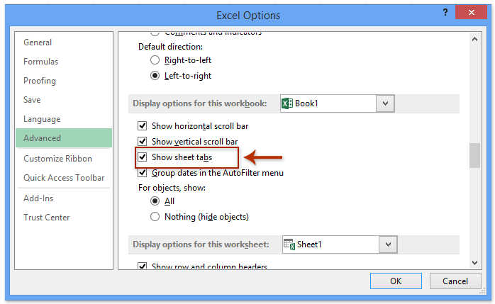
- Scroll down to the ‘Display Options for this Workbook’ section
- Check the ‘Show sheet tabs’ option

The above change would ensure that all the available sheet tabs in the workbook become visible (unless the user has specifically hidden some of the worksheets)
Note that this setting is workbook specific – which means that in case you enable this setting in one of the workbooks, it would only make the tabs reappear in that specific workbook
When Some of the Sheet Tabs are Missing
Sometimes, you may be able to see some of the tabs in the workbook, while some others may be missing.
In this section, I have some solutions when only some of the tabs are missing and some are visible.
Some of the Sheets are Hidden
The most likely reason that you cannot see some of the tabs in the workbook is that they have been hidden by the user.
When a worksheet is hidden in Excel, it continues to exist as a part of the Excel workbook, but you don’t see that sheet tab name along with other sheet tabs.
And this has a really simple solution – you need to unhide the sheets.
Below are the steps to unhide one or more sheets in Excel:
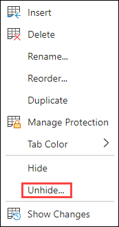
- Right-click on any of the existing sheet tab name
- Click on the Unhide option. In case there are no hidden sheets in the workbook, this option will be grayed out

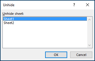
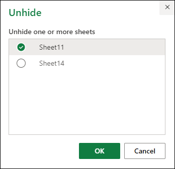
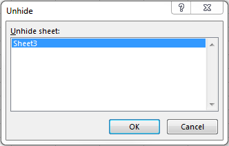
- In the Unhide dialog box, click on the sheet name you want to unhide

- Click on OK

The above steps would unhide the selected sheet, and it would reappear as a tab in your workbook.
In case you want to unhide multiple sheets, you can select them in one go in the ‘Unhide’ dialog box. To do this, hold the Control key (or Command key if using Mac) and then click on the Sheet names that you want to unhide. This would select all the sheets on which you click and then you can unhide all these with one click.
But what if you do not see the tab name in the names listed in the Unhide dialog box?
Well, there is a way in Excel to hide a sheet in such a way that its name doesn’t show up in the Unhide dialog box.
Then how do you unhide these ‘very hidden’ sheets?
You can read my tutorial here where I show you how to unhide those sheets that have been ‘very hidden’. It’s easy and it will only take a couple of clicks.
Tabs are Hidden Because of the Scroll Bar
Another reason your tabs may be missing could be because of a large scroll bar that hides the tabs.
And it has a simple fix – resize the scroll bar to make all other tabs visible.
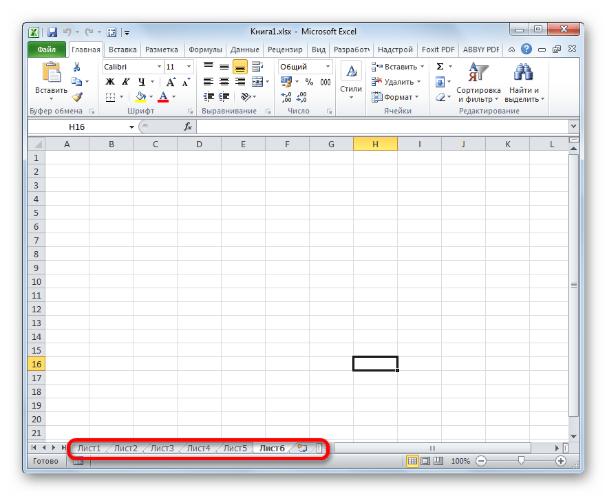
Below I have a screenshot of an Excel workbook where I have 8 sheets but only three sheet tabs are visible. This is because of a large scrollbar that hides those tab names.

To get the sheet tabs to reappear, click on the three dots icon on the left of the scrollbar and drag it to the right. This will minimize the scroll bar and all the sheet tabs that were earlier hidden would now become visible.

In case you have a large workbook with a lot of sheets, even if you minimize the scrollbar, some sheet tabs would still be hidden.
In such a case, you can use the navigation icons (which are at the left of the first sheet tab) to make those sheet tabs visible.
So these are some of the ways you can use to fix the issue when the sheet tabs are missing and not showing in Excel. If you don’t see any sheet tab in the workbook, it’s most likely because of the setting in the Excel Options dialog box that needs to be changed.
And in case you see some sheet tab names but some are missing, then you need to check if some of the sheets have been hidden by the user or if they are hidden because of a large scroll bar.
Other Excel tutorials you may also like:
- Microsoft Excel Won’t Open – How to Fix it! (6 Possible Solutions)
- How to Switch Between Sheets in Excel? (7 Better Ways)
- Count Sheets in Excel (using VBA)
- How to Get the Sheet Name in Excel? Easy Formula
- How to Insert New Worksheet in Excel (Easy Shortcuts)
- How to Delete Sheets in Excel (Shortcuts + VBA)
- Arrow Keys not Working in Excel | Moving Pages Instead of Cells
- How to Change the Color of the Sheet Tab in Excel
Last Update: Jan 03, 2023
This is a question our experts keep getting from time to time. Now, we have got the complete detailed explanation and answer for everyone, who is interested!
Asked by: Prof. Stanley Spinka
Score: 4.6/5
(31 votes)
The Show sheet tabs setting is turned off. First ensure that the Show sheet tabs is enabled. To do this, For all other Excel versions, click File > Options > Advanced—in under Display options for this workbook—and then ensure that there is a check in the Show sheet tabs box.
How do I see all sheets in Excel?
Excel: Right Click to Show a Vertical Worksheets List
- Right-click the controls to the left of the tabs.
- You’ll see a vertical list displayed in an Activate dialog box. Here, all sheets in your workbook are shown in an easily accessed vertical list.
- Click on whatever sheet you need and you’ll instantly see it!
Why Excel file is open but not visible?
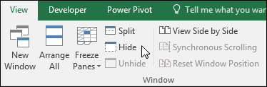
However, sometimes when you open a workbook, you see that it is open but you can’t actually see it. This could be as a result of an intentional or accidental hiding of the workbook (as apposed to a sheet). Under the VIEW tab you will see buttons called Hide and Unhide.
Where did my Excel sheet go?
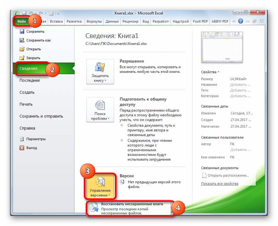
Step 1 — Open Excel, click «File» and then click «Info.» Click the «Manage Versions» button and then choose «Recover Unsaved Workbooks» from the menu. Step 2 — Select the file to restore and then click «Open» to load the workbook. Step 3 — Click the «Save As» button on the yellow bar to recover the worksheet.
How do I view hidden sheets in Excel?
Unhide Worksheets Using the Ribbon
- Select one or more worksheet tabs at the bottom of the Excel file.
- Click the Home tab on the ribbon.
- Select Format.
- Click Hide & Unhide.
- Select Unhide Sheet.
- Click the sheet you want to unhide from the list that pops up.
- Click OK.
37 related questions found
How do I unhide all sheets?
Unhide multiple worksheets
- Right-click the Sheet tab at the bottom, and select Unhide.
- In the Unhide dialog box, — Press the Ctrl key (CMD on Mac) and click the sheets you want to show, or. — Press the Shift + Up/Down Arrow keys to select multiple (or all) worksheets, and then press OK.
How do I view hidden sheets in Excel 2016?
MS Excel 2016: Unhide a sheet
- To unhide Sheet2, right-click on the name of any sheet and select Unhide from the popup menu.
- When the Unhide window appears, it will list all of the hidden sheets. Select the sheet that you wish to unhide. …
- Now when you return to your spreadsheet, Sheet2 should be visible.
- NEXT.
How do I add a sheet in Excel?
On the Home tab, in the Cells group, click Insert, and then click Insert Sheet. Tip: You can also right-click the selected sheet tabs, and then click Insert. On the General tab, click Worksheet, and then click OK.
Why did my Excel file disappear?
If your Excel file disappeared. Sudden power failure can cause your Excel spreadsheet not to be saved and probably disappear from your computer. Also, if Excel is not responding and then it is forced to close, the current spreadsheet being worked on may not be saved.
Why does my Excel sheet disappear when I minimize?
Since when a Window is sized (click the Arrange button in the Window Group on the View tab), it can be dragged down, the worksheet tabs might seem to disappear. … It is now maximized inside the application window and your worksheet tabs should once again be accessible.
How do I unhide hidden sheets in Excel?
Hide or Unhide worksheets
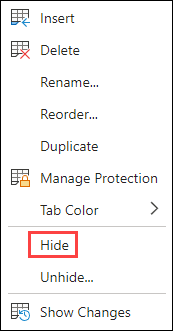
- Right-click the sheet tab you want to hide, or any visible sheet if you want to unhide sheets.
- On the menu that appears, do one of the following: To hide the sheet, select Hide. To unhide hidden sheets, select them in the Unhide dialog that appears, and then select OK.
How do I view all sheets in Excel 2010?
How to Display Sheet Tabs in Excel 2010
- Open Excel.
- Click File.
- Choose Options.
- Select the Advanced tab.
- Check the box to the left of Show sheet tabs.
- Click OK.
How do I stop text from disappearing in Excel?
Hold Ctrl+A > Click Format > Font and make sure Hidden is not checked.
How do you unhide data in Excel?
To unhide all of the cells in a worksheet:
- Click the Select All button, in the upper-left corner of the worksheet or press Ctrl + A.
- Click the Home tab > Format (in the Cells group) > Hide & Unhide > Unhide Rows or Unhide Columns.
- All cells are now visible.
Where is the new sheet button in Excel?
To insert a single new worksheet to the right of the currently selected worksheet, click the “New Sheet” button at the right end of the spreadsheet name tabs. Alternatively, click the “Insert” drop-down button in the “Cells” button group on the “Home” tab of the Ribbon.
How many sheets can you have in Excel?
How many sheets are there in an Excel workbook? By default, there are three sheets in a new workbook in all versions of Excel, though users can create as many as their computer memory allows. These three worksheets are named Sheet1, Sheet2, and Sheet3.
How do I add a sheet in Excel using the keyboard?
SHIFT + F11 is the shortcut key to insert a new worksheet. Ctrl + Drag will create the replica of the existing worksheet, and the only changes are sheet name.
How unhide a column in Excel?
Unhide columns
- Select the adjacent columns for the hidden columns.
- Right-click the selected columns, and then select Unhide.
Why is Excel not Unhiding rows?
If you select all the rows and click ‘unhide’ and they do not show up, then they are filtered and not hidden. Click the Sort & Filter button on the Home tab of the ribbon and then click ‘clear’. … On the Home tab, click on the Format icon Choose Hide & Unhide from the dropdown menu then select Unhide Rows.
How do I unhide all columns in an Excel spreadsheet?
How to unhide columns in Excel:
- Click on the small green triangle in the top left corner of your spreadsheet. This will select the entire spreadsheet.
- Now right-click anywhere in the entire selection and choose the Unhide option from the menu.
- You should now be able to see all of your columns.
Why is my text invisible in Excel?
Workaround 2 – Change the Default Font
The font of cells in your Excel worksheet may be creating the problem. So, try changing the default font of cells or ranges: Select a cell or cell range where the text is not showing up. Right-click on the selected cell or cell range and click Format Cells.
Why does my typing disappear?
Turn off overtype mode: Click File > Options. Click Advanced. Under Editing options, clear both the Use the Insert key to control overtype mode and the Use overtype mode check boxes.
How do I view hidden sheets in Excel 2010?
1Click anywhere on the worksheet that you want to hide. 2In the Cells group on the Home tab, choose Format→Hide & Unhide→Hide Sheet. 3To unhide the worksheet, choose Format→Hide & Unhide→Unhide Sheet. 4Select the worksheet you want to unhide and click OK.
How do you make a sheet visible?
To unhide a sheet, simply right-click any sheet’s tab and select Unhide. This reveals the Unhide dialog box as shown below. Pick the hidden sheet and click ok.
Ever stuck into such an issue where you can’t see tabs in Excel or sheets not visible in Excel? Looking for some easy tricks to fix Excel tabs not showing issue?
Leave all you worry because, for easy restoration of missing worksheet tabs, this tutorial is surely going to help you a lot. Here you will get the best tricks to overcome the Excel spreadsheets disappeared issue in an easy way.
Apart from that, you will also get an easy idea of how to find hidden worksheets in Excel 2010/2013/2016/2019.
Why Did My Excel Worksheet Disappeared?

Normally, within the Excel workbook, you will get several tabs along with the bottom of the screen. The missing Excel worksheet tab issue mainly generates when sheets may get hidden in plain sight due to some changes in the Excel setting.
In order to solve the mystery of Excel tabs not showing problems let’s first find the answer to why are tabs not showing in Excel? After then follow the workarounds to fix the Excel missing sheet tabs issue.
There are numerous things that will make your Excel sheet disappeared.
Here we have listed some most common causes of Excel sheet tabs missing. Have a Look…
- When you inadvertently disconnect the workbook Windows from Excel. Mainly while using the trio of restore windows buttons on the title bar and moving the Windows under the status bar.
- The screen resolution is done too high and the tab gets vanished from the bottom of the screen.
- You may have turned off the Display options for this workbook.
- The workbook window is sized in a way that the tabs are hidden.
- The tabs get obscure due to the horizontal scroll bar.
- The worksheet itself is hidden.
How To Fix Excel Tabs Not Showing Issue?

Follow the given methods to troubleshoot Excel Tabs Not Showing issue:
1: Change the Zoom Settings
2: Check Show Sheet Tabs Setting Is Turned Off
3: Unhide the Worksheet
4: Check The Show Sheet Tabs Settings Controls
5: Check Excel Windows Arrangement
6: Click the Navigation Arrow in the Excel File
Now it’s time to discuss each of these methods of fixing Excel Worksheet disappeared in detail. So, let’s get started….!
Watch out this interesting video on how to restore missing Excel worksheet tabs and cells.
Method 1: Change the Zoom Settings
Change the zoom settings to some other settings. Then change the zoom settings back to the preferred settings.
Follow these steps to do this:
- Click the zoom out or zoom in on the status bar.
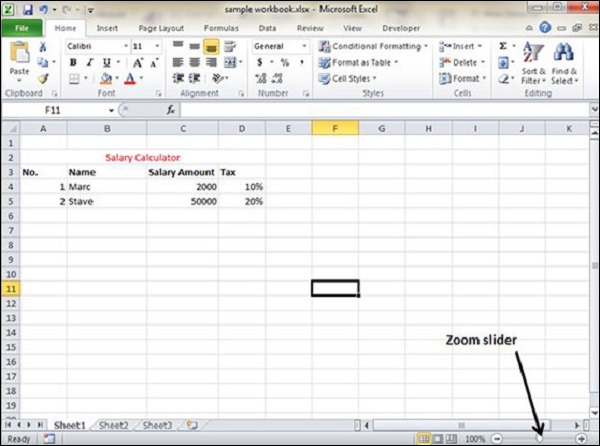
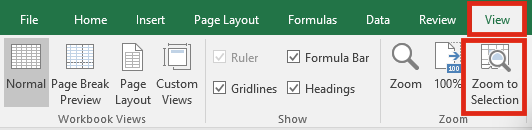
- On the View tab, click zoom in the zoom group, select the settings you want under Magnification, and then click OK.
Hope by changing the zoom settings you are able to see the missing Excel sheet tabs but if not then follow the method 2
Method 2: Check Show Sheet Tabs Setting Is Turned Off
This might be the case that Excel sheet tabs go missing as the sheet tabs setting is turned off. To verify it, follow the steps to do so:
- Click File > Options > Advanced, then under Display options for this workbook.
- Assure that the Show sheet tab checkbox is selected.
This process is the same for all Excel versions.
Method 3: Unhide the Worksheet
In many cases, the Excel sheet disappeared by itself. So to get the missing sheet tab back you must use the unhide worksheet of Excel.
Follow the steps to do so:
- Right-click on any visible tab on the worksheet > click Unhide
- Then in the Unhide dialog box > click sheet you desire to unhide
- Click Ok.

Method 4: Check The Show Sheet Tabs Settings Controls
In Excel 2010 and former, it is comparatively easy to unintentionally organize a spreadsheet Window. Subsequently, the worksheet tabs aren’t present on the screen, even if the Show Sheet Tabs option is enabled. While this happens, double click on the workbook’s name to maximize the Window and recover workbooks.
In Excel 2013 if you are not able to see the worksheet tabs, simply double-click on the words “Microsoft Excel” at the top of the Windows for maximizing Excel’s application window.

Method 5: Check Excel Windows Arrangement
In some cases, it is found that Excel Windows get arranged in such a way so that the tabs are not visible. So check for them. Make use of the keyboard shortcut to navigate between worksheets within the workbook. And to do this, press Ctrl – Page Up for activating the adjacent worksheets to the left and or else press Ctrl- Page Down for activating the next worksheet to the right.

In this activate menu Excel 2013 provides helpful improvements since the entire worksheets are displayed in a single dialog box and after that, you can select a worksheet by entering the first letter of the sheet name.
In Excel 2010 or the earlier version, the Activate menu very first displays up to 16 worksheets and requires selecting more sheets for displaying more lists.
Additionally, in Excel 2010 or the earlier version, you should select the desired sheet name by making use of your mouse. Because the menu cannot be accessed by way of keystrokes as it is possible in Excel 2013.
You can also read: 7 Tricks To Fix Missing Gridlines In Excel Issue
Method 6: Click the Navigation Arrow in the Excel File

In many other cases, it happens that the worksheet tabs are available, but a worksheet still appears missing. In Excel 2007 and later versions, right-click on any worksheet tab and select unhide.
Well, if the command is disabled there is most likely no hidden worksheet is present in the workbook. However, there is still a way you can find out this possibility.
Follow the steps to access the unhide sheet command from Excel’s main menu:
- Excel 2007 and later: Go to the home tab > select format > click hide and unhide sheet.

- Excel 2003 and earlier: Select Format > Sheet > and Unhide.
- And Excel 2011 for Mac: From the main menu > select format option > sheet > unhide. The format command on the home tab of the ribbon doesn’t let you unhide the worksheet.
If the unhide sheet is disabled, you can’t necessarily assume that there are no hidden worksheets within a workbook.
Automatic Solution To Recover Missing/Disappeared Tabs In Excel
Well, if none of the above-mentioned methods help you to recover missing sheets in Excel. Then the chances are high that your Excel sheet has caught into some corruption issue. Due to the corruption of the Excel sheet, you may also find that your Excel sheet content disappeared.
In this case, you can make use of the professional recommended MS Excel Repair Tool. This is the best tool to repair any sort of issues, corruption as well as errors in Excel files. It also restores the entire data in the preferred location. It is too easy to use.
* Free version of the product only previews recoverable data.
Steps to Utilize MS Excel Repair Tool:
Conclusion:
Hope after reading the article you are able to recover your missing sheet tabs in Excel. I tried my best to provide complete information about how to recover the missing or hidden sheet tabs in Microsoft Excel.
So, now it’s your turn to make use of the given methods to fix Excel tabs not showing the issue. Just go for it.
Good Luck!!!


Priyanka is an entrepreneur & content marketing expert. She writes tech blogs and has expertise in MS Office, Excel, and other tech subjects. Her distinctive art of presenting tech information in the easy-to-understand language is very impressive. When not writing, she loves unplanned travels.
Hide or unhide a worksheet
Note: The screen shots in this article were taken in Excel 2016. If you have a different version your view might be slightly different, but unless otherwise noted, the functionality is the same.
-
Select the worksheets that you want to hide.
How to select worksheets
To select
Do this
A single sheet
Click the sheet tab.

If you don’t see the tab that you want, click the scrolling buttons to the left of the sheet tabs to display the tab, and then click the tab.
Two or more adjacent sheets
Click the tab for the first sheet. Then hold down Shift while you click the tab for the last sheet that you want to select.
Two or more nonadjacent sheets
Click the tab for the first sheet. Then hold down Ctrl while you click the tabs of the other sheets that you want to select.
All sheets in a workbook
Right-click a sheet tab, and then click Select All Sheets on the shortcut menu.
Tip: When multiple worksheets are selected, [Group] appears in the title bar at the top of the worksheet. To cancel a selection of multiple worksheets in a workbook, click any unselected worksheet. If no unselected sheet is visible, right-click the tab of a selected sheet, and then click Ungroup Sheets on the shortcut menu.
-
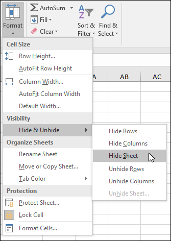
On the Home tab, in the Cells group, click Format > Visibility > Hide & Unhide > Hide Sheet.
-
To unhide worksheets, follow the same steps, but select Unhide. You’ll be presented with a dialog box listing which sheets are hidden, so select the ones you want to unhide.
Note: Worksheets hidden by VBA code have the property xlSheetVeryHidden; the Unhide command will not display those hidden sheets. If you are using a workbook that contains VBA code and you encounter problems with hidden worksheets, contact the workbook owner for more information.

Hide or unhide a workbook window
-
On the View tab, in the Window group, click Hide or Unhide.
On a Mac, this is under the Window menu in the file menu above the ribbon.
Notes:
-
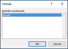
When you Unhide a workbook, select from the list in the Unhide dialog box.
-
If Unhide is unavailable, the workbook does not contain hidden workbook windows.
-
When you exit Excel, you will be asked if you want to save changes to the hidden workbook window. Click Yes if you want the workbook window to be the same as you left it (hidden or unhidden), the next time that you open the workbook.
Hide or display workbook windows on the Windows taskbar
Excel 2013 introduced the Single Document Interface, where each workbook opens in its own window.
-
Click File > Options.
For Excel 2007, click the Microsoft Office Button
, then Excel Options. -
Then click Advanced > Display > clear or select the Show all windows in the Taskbar check box.
 , then Excel Options.
Hide or unhide a worksheet
-
Select the worksheets that you want to hide.
How to select worksheets
To select
Do this
A single sheet
Click the sheet tab.
If you don’t see the tab that you want, click the scrolling buttons to the left of the sheet tabs to display the tab, and then click the tab.
Two or more adjacent sheets
Click the tab for the first sheet. Then hold down Shift while you click the tab for the last sheet that you want to select.
Two or more nonadjacent sheets
Click the tab for the first sheet. Then hold down Command while you click the tabs of the other sheets that you want to select.
All sheets in a workbook
Right-click a sheet tab, and then click Select All Sheets on the shortcut menu.
-
On the Home tab, click Format > under Visibility > Hide & Unhide > Hide Sheet.
-
To unhide worksheets, follow the same steps, but select Unhide. The Unhide dialog box displays a list of hidden sheets, so select the ones you want to unhide and then select OK.
Hide or unhide a workbook window
-
Click the Window menu, click Hide or Unhide.
Notes:
-
When you Unhide a workbook, select from the list of hidden workbooks in the Unhide dialog box.
-
If Unhide is unavailable, the workbook does not contain hidden workbook windows.
-
When you exit Excel, you will be asked if you want to save changes to the hidden workbook window. Click Yes if you want the workbook window to be the same as you left it (hidden or unhidden) the next time that you open the workbook.
Hide a worksheet
-
Right click on the tab you want to hide.
-
Select Hide.
Unhide a worksheet
-
Right click on any visible tab.
-
Select Unhide.
-
Mark the tabs to unhide.
-
Click OK.
Содержание
- Восстановление листов
- Способ 1: включение панели ярлыков
- Способ 2: перемещения полосы прокрутки
- Способ 3: включение показа скрытых ярлыков
- Способ 4: отображение суперскрытых листов
- Способ 5: восстановление удаленных листов
- Вопросы и ответы
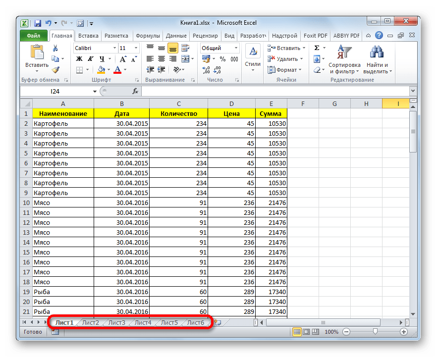
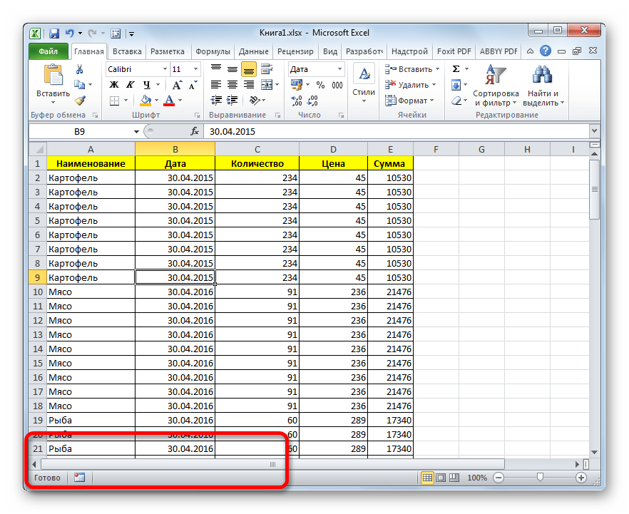
Возможность в Экселе создавать отдельные листы в одной книге позволяет, по сути, формировать несколько документов в одном файле и при необходимости связывать их ссылками или формулами. Конечно, это значительно повышает функциональность программы и позволяет расширить горизонты поставленных задач. Но иногда случается, что некоторые созданные вами листы пропадают или же полностью исчезают все их ярлыки в строке состояния. Давайте выясним, как можно вернуть их назад.
Восстановление листов
Навигацию между листами книги позволяют осуществлять ярлыки, которые располагаются в левой части окна над строкой состояния. Вопрос их восстановления в случае пропажи мы и будем рассматривать.
Прежде, чем приступить к изучению алгоритма восстановления, давайте разберемся, почему они вообще могут пропасть. Существуют четыре основные причины, почему это может случиться:
- Отключение панели ярлыков;
- Объекты были спрятаны за горизонтальной полосой прокрутки;
- Отдельные ярлыки были переведены в состояние скрытых или суперскрытых;
- Удаление.
Естественно, каждая из этих причин вызывает проблему, которая имеет собственный алгоритм решения.
Способ 1: включение панели ярлыков
Если над строкой состояния вообще отсутствуют ярлыки в положенном им месте, включая ярлык активного элемента, то это означает, что их показ попросту был кем-то отключен в настройках. Это можно сделать только для текущей книги. То есть, если вы откроете другой файл Excel этой же программой, и в нем не будут изменены настройки по умолчанию, то панель ярлыков в нем будет отображаться. Выясним, каким образом можно снова включить видимость в случае отключения панели в настройках.
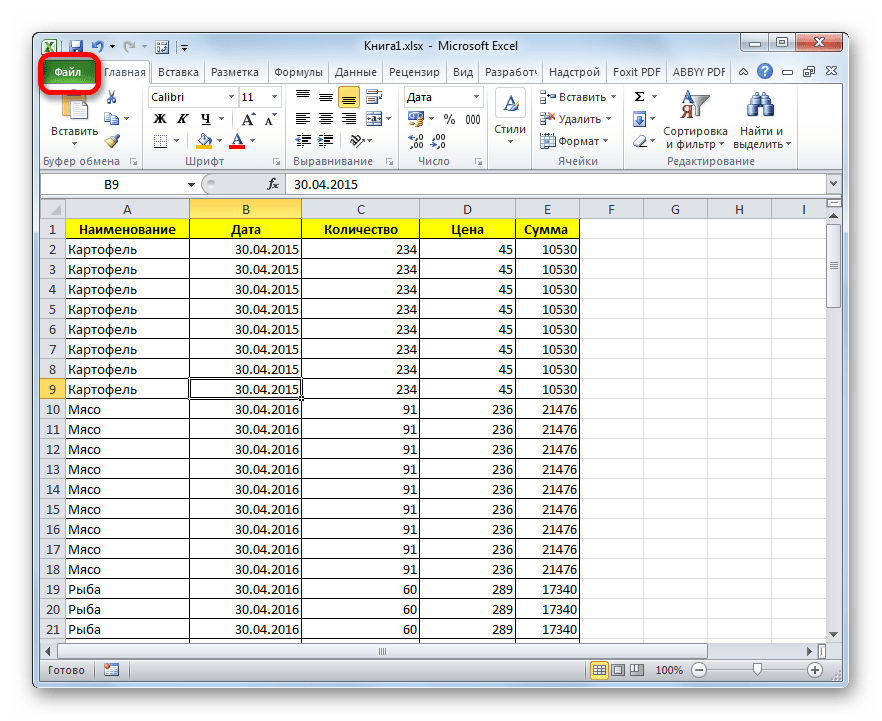
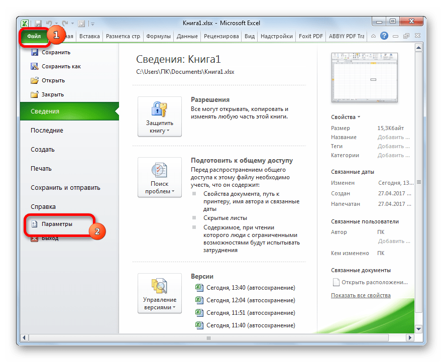
- Переходим во вкладку «Файл».
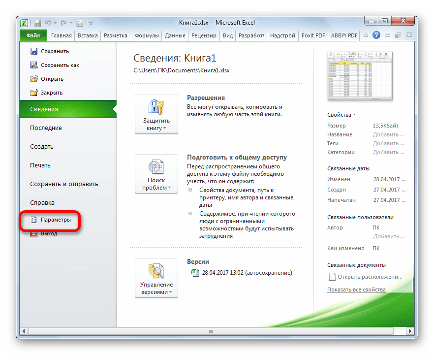
- Далее производим перемещение в раздел «Параметры».
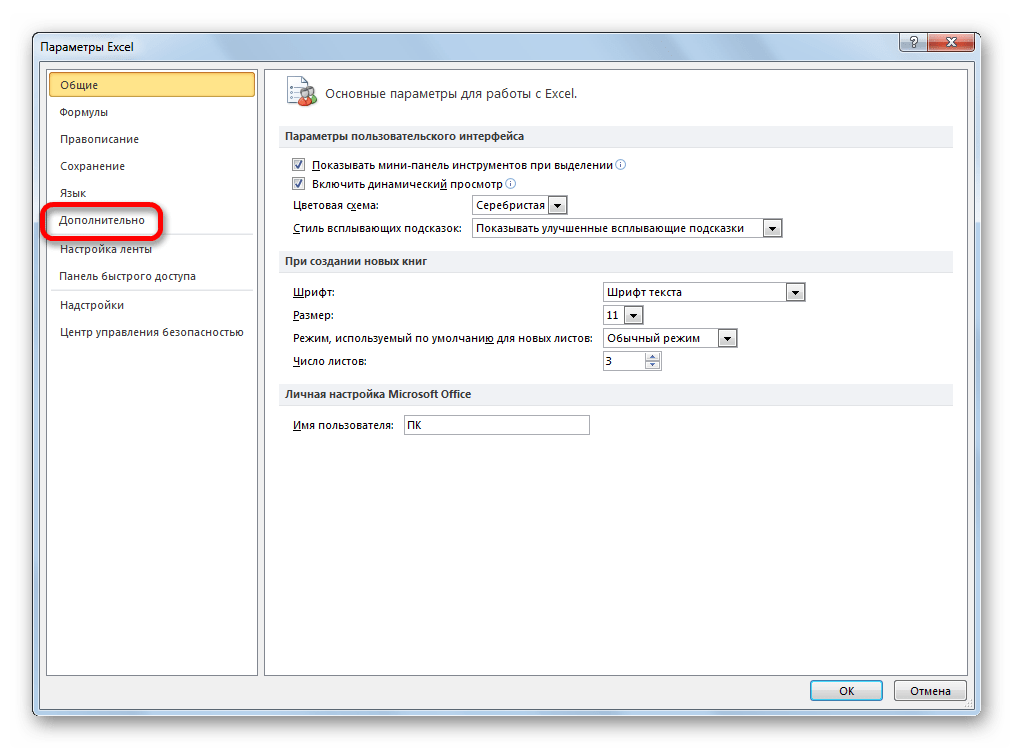
- В открывшемся окне параметров Excel выполняем переход во вкладку «Дополнительно».
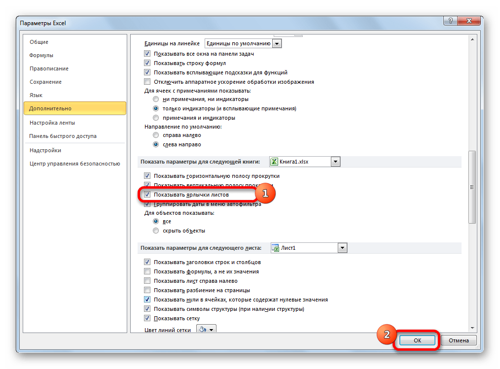
- В правой части открывшегося окна располагаются различные настройки Excel. Нам нужно найти блок настроек «Показывать параметры для следующей книги». В этом блоке имеется параметр «Показывать ярлычки листов». Если напротив него отсутствует галочка, то следует её установить. Далее щелкаем по кнопке «OK» внизу окна.
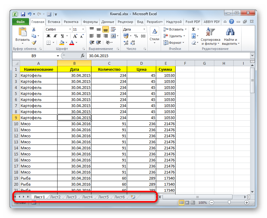
- Как видим, после выполнения указанного выше действия панель ярлыков снова отображается в текущей книге Excel.
Способ 2: перемещения полосы прокрутки
Иногда бывают случаи, когда пользователь случайно перетянул горизонтальную полосу прокрутки поверх панели ярлыков. Тем самым он фактически скрыл их, после чего, когда обнаруживается данный факт, начинается лихорадочный поиск причины отсутствия ярлычков.
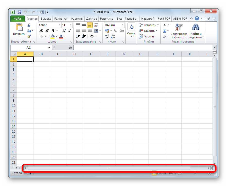

- Решить данную проблему очень просто. Устанавливаем курсор слева от горизонтальной полосы прокрутки. Он должен преобразоваться в двунаправленную стрелку. Зажимаем левую кнопку мыши и тащим курсор вправо, пока не будут отображены все объекты на панели. Тут тоже важно не переборщить и не сделать полосу прокрутки слишком маленькой, ведь она тоже нужна для навигации по документу. Поэтому следует остановить перетаскивание полосы, как только вся панель будет открыта.
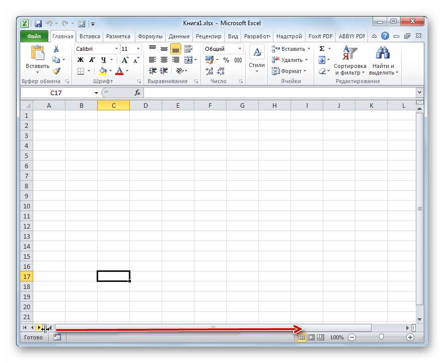
- Как видим, панель снова отображается на экране.
Способ 3: включение показа скрытых ярлыков
Также отдельные листы можно скрыть. При этом сама панель и другие ярлыки на ней будут отображаться. Отличие скрытых объектов от удаленных состоит в том, что при желании их всегда можно отобразить. К тому же, если на одном листе имеются значения, которые подтягиваются через формулы расположенные на другом, то в случае удаления объекта эти формулы начнут выводить ошибку. Если же элемент просто скрыть, то никаких изменений в функционировании формул не произойдет, просто ярлыки для перехода будут отсутствовать. Говоря простыми словами, объект фактически останется в том же виде, что и был, но инструменты навигации для перехода к нему исчезнут.
Процедуру скрытия произвести довольно просто. Нужно кликнуть правой кнопкой мыши по соответствующему ярлыку и в появившемся меню выбрать пункт «Скрыть».
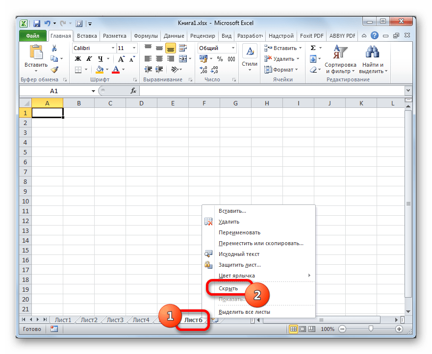
Как видим, после этого действия выделенный элемент будет скрыт.
Теперь давайте разберемся, как отобразить снова скрытые ярлычки. Это не намного сложнее, чем их спрятать и тоже интуитивно понятно.
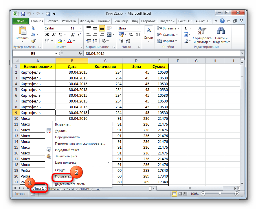
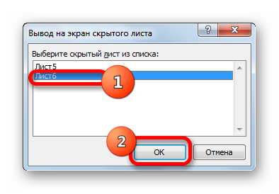
- Кликаем правой кнопкой мыши по любому ярлыку. Открывается контекстное меню. Если в текущей книге имеются скрытые элементы, то в данном меню становится активным пункт «Показать…». Щелкаем по нему левой кнопкой мыши.
- После клика происходит открытие небольшого окошка, в котором расположен список скрытых листов в данной книге. Выделяем тот объект, который снова желаем отобразить на панели. После этого щелкаем по кнопке «OK» в нижней части окошка.
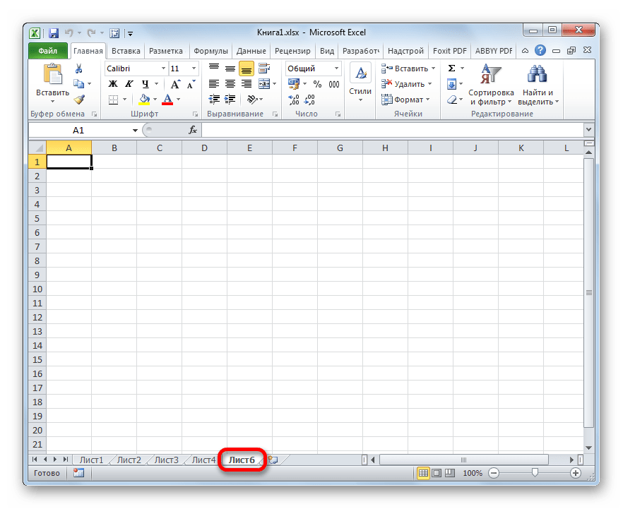
- Как видим, ярлычок выбранного объекта снова отобразился на панели.
Способ 4: отображение суперскрытых листов
Кроме скрытых листов существуют ещё суперскрытые. От первых они отличаются тем, что вы их не найдете в обычном списке вывода на экран скрытого элемента. Даже в том случае, если уверены, что данный объект точно существовал и никто его не удалял.
Исчезнуть данным образом элементы могут только в том случае, если кто-то их целенаправленно скрыл через редактор макросов VBA. Но найти их и восстановить отображение на панели не составит труда, если пользователь знает алгоритм действий, о котором мы поговорим ниже.
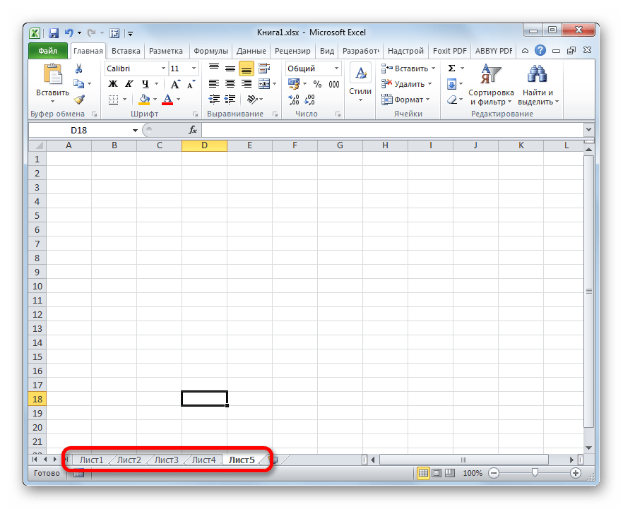
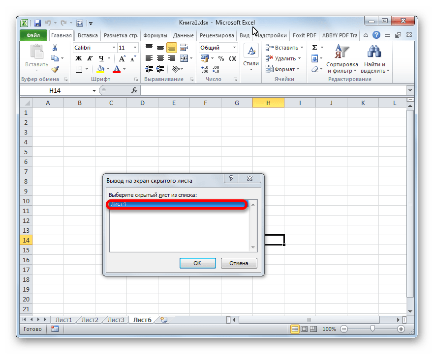
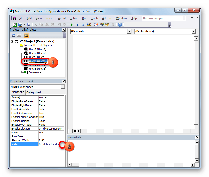
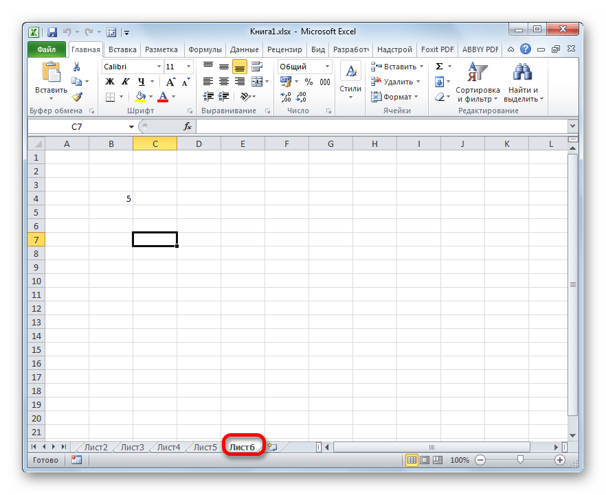
В нашем случае, как мы видим, на панели отсутствуют ярлычки четвертого и пятого листа.
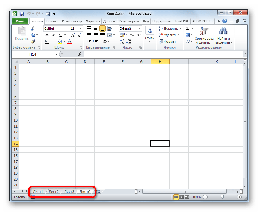
Перейдя в окошко вывода на экран скрытых элементов, тем путем, о котором мы говорили в предыдущем способе, видим, что в нем отображается только наименование четвертого листа. Поэтому, вполне очевидно предположить, что если пятый лист не удален, то он скрыт посредством инструментов редактора VBA.
- Прежде всего, нужно включить режим работы с макросами и активировать вкладку «Разработчик», которые по умолчанию отключены. Хотя, если в данной книге некоторым элементам был присвоен статус суперскрытых, то не исключено, что указанные процедуры в программе уже проведены. Но, опять же, нет гарантии того, что после выполнения скрытия элементов пользователь, сделавший это, опять не отключил необходимые инструменты для включения отображения суперскрытых листов. К тому же, вполне возможно, что включение отображения ярлыков выполняется вообще не на том компьютере, на котором они были скрыты.
Переходим во вкладку «Файл». Далее кликаем по пункту «Параметры» в вертикальном меню, расположенном в левой части окна.
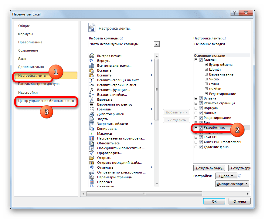
- В открывшемся окне параметров Excel щелкаем по пункту «Настройка ленты». В блоке «Основные вкладки», который расположен в правой части открывшегося окна, устанавливаем галочку, если её нет, около параметра «Разработчик». После этого перемещаемся в раздел «Центр управления безопасностью» с помощью вертикального меню в левой части окна.
- В запустившемся окне щелкаем по кнопке «Параметры центра управления безопасностью…».
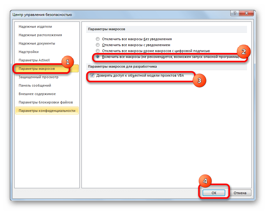
- Производится запуск окна «Центр управления безопасностью». Переходим в раздел «Параметры макросов» посредством вертикального меню. В блоке инструментов «Параметры макросов» устанавливаем переключатель в позицию «Включить все макросы». В блоке «Параметры макросов для разработчика» устанавливаем галочку около пункта «Доверять доступ к объектной модели проектов VBA». После того, как работа с макросами активирована, жмем на кнопку «OK» внизу окна.
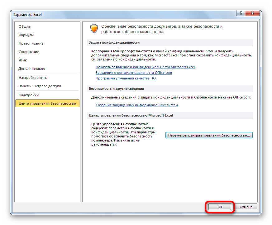
- Вернувшись к параметрам Excel, чтобы все изменения настроек вступили в силу, также жмем на кнопку «OK». После этого вкладка разработчика и работа с макросами будут активированы.
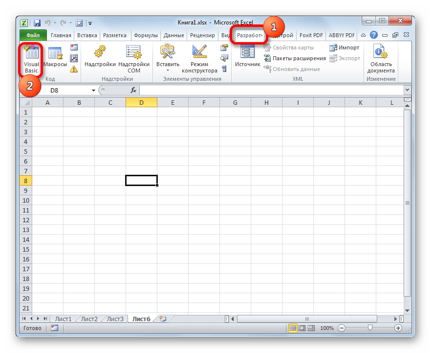
- Теперь, чтобы открыть редактор макросов, перемещаемся во вкладку «Разработчик», которую мы только что активировали. После этого на ленте в блоке инструментов «Код» щелкаем по большому значку «Visual Basic».

Редактор макросов также можно запустить, набрав на клавиатуре сочетание клавиш Alt+F11.
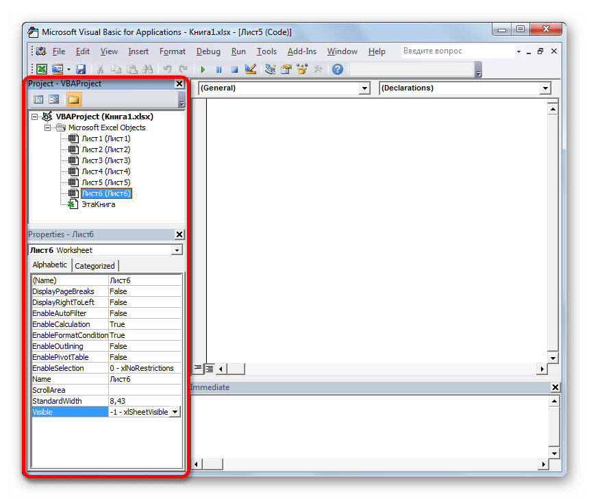
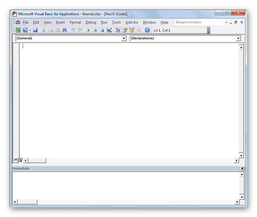
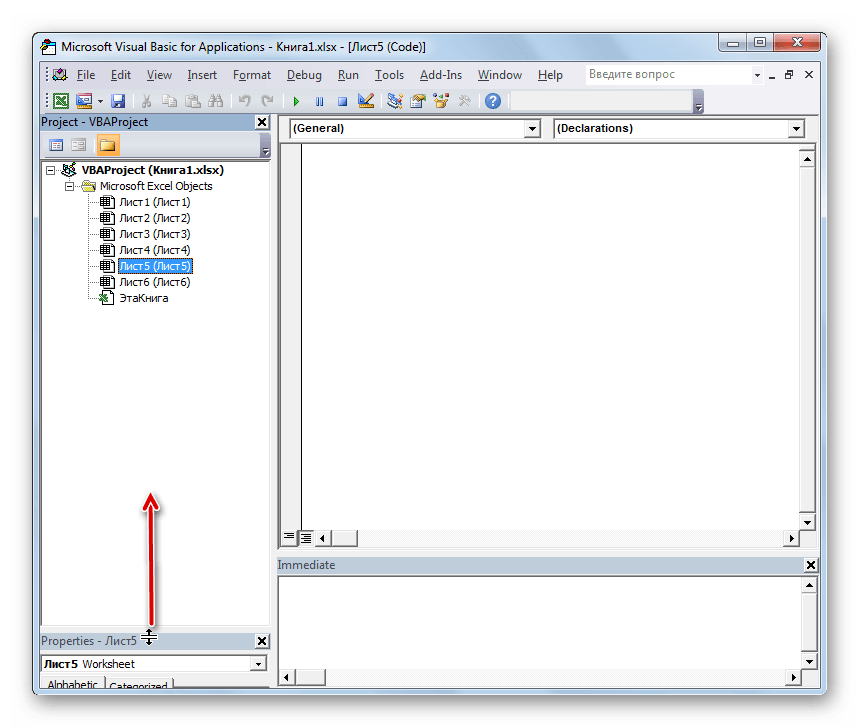
- После этого откроется окно редактора макросов, в левой части которого расположены области «Project» и «Properties».

Но вполне возможно, что данных областей не окажется в открывшемся окне.
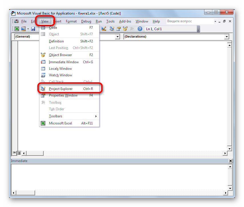
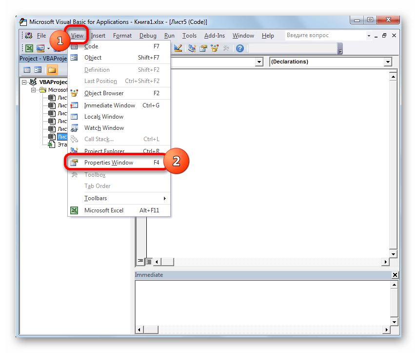
- Для включения отображения области «Project» щелкаем по пункту горизонтального меню «View». В открывшемся списке выбираем позицию «Project Explorer». Либо же можно произвести нажатие сочетания горячих клавиш Ctrl+R.
- Для отображения области «Properties» опять кликаем по пункту меню «View», но на этот раз в списке выбираем позицию «Properties Window». Или же, как альтернативный вариант, можно просто произвести нажатие на функциональную клавишу F4.
- Если одна область перекрывает другую, как это представлено на изображении ниже, то нужно установить курсор на границе областей. При этом он должен преобразоваться в двунаправленную стрелку. Затем зажать левую кнопку мыши и перетащить границу так, чтобы обе области полностью отображались в окне редактора макросов.
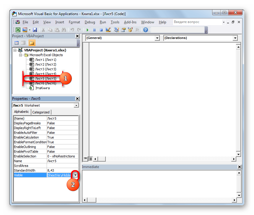
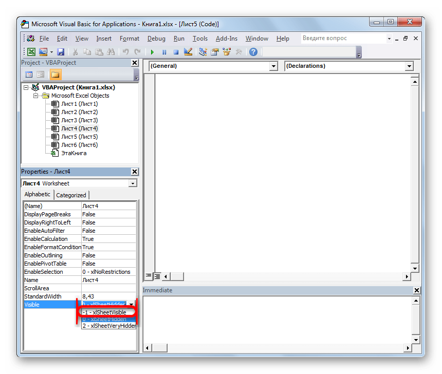
- После этого в области «Project» выделяем наименование суперскрытого элемента, который мы не смогли отыскать ни на панели, ни в списке скрытых ярлыков. В данном случае это «Лист 5». При этом в области «Properties» показываются настройки данного объекта. Нас конкретно будет интересовать пункт «Visible» («Видимость»). В настоящее время напротив него установлен параметр «2 — xlSheetVeryHidden». В переводе на русский «Very Hidden» означает «очень скрытый», или как мы ранее выражались «суперскрытый». Чтобы изменить данный параметр и вернуть видимость ярлыку, кликаем на треугольник справа от него.
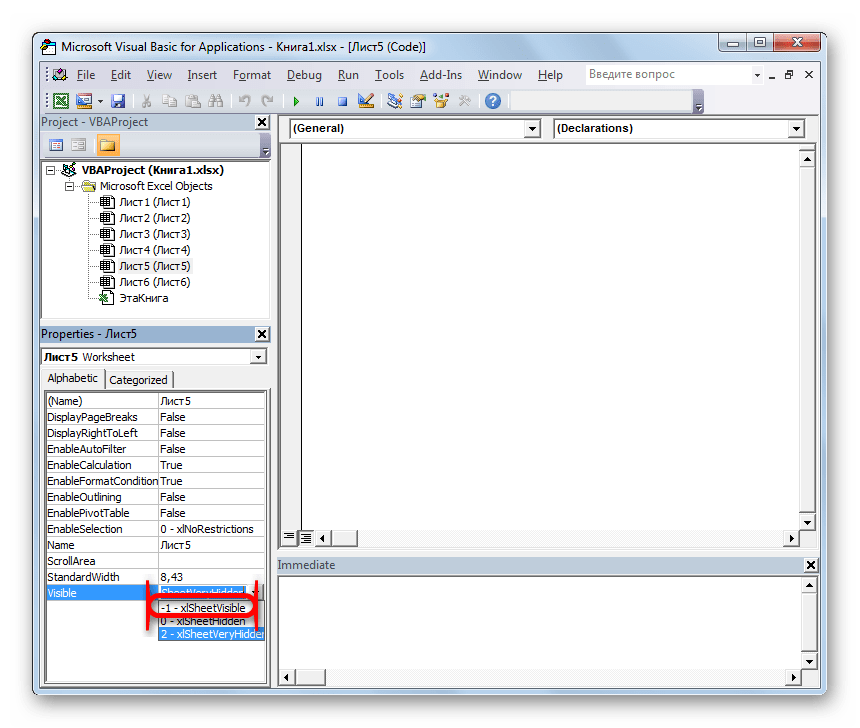
- После этого появляется список с тремя вариантами состояния листов:
- «-1 – xlSheetVisible» (видимый);
- «0 – xlSheetHidden» (скрытый);
- «2 — xlSheetVeryHidden» (суперскрытый).
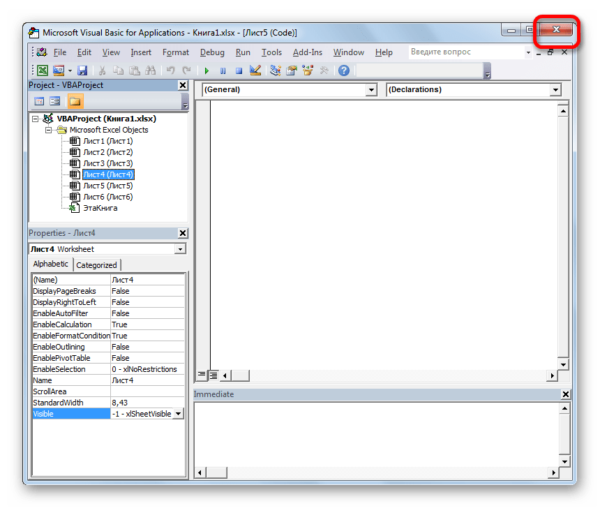
Для того, чтобы ярлык снова отобразился на панели, выбираем позицию «-1 – xlSheetVisible».
- Но, как мы помним, существует ещё скрытый «Лист 4». Конечно, он не суперскрытый и поэтому отображение его можно установить при помощи Способа 3. Так даже будет проще и удобнее. Но, если мы начали разговор о возможности включения отображения ярлыков через редактор макросов, то давайте посмотрим, как с его помощью можно восстанавливать обычные скрытые элементы.
В блоке «Project» выделяем наименование «Лист 4». Как видим, в области «Properties» напротив пункта «Visible» установлен параметр «0 – xlSheetHidden», который соответствует обычному скрытому элементу. Щелкаем по треугольнику слева от данного параметра, чтобы изменить его.
- В открывшемся списке параметров выбираем пункт «-1 – xlSheetVisible».
- После того, как мы настроили отображение всех скрытых объектов на панели, можно закрывать редактор макросов. Для этого щелкаем по стандартной кнопке закрытия в виде крестика в правом верхнем углу окна.
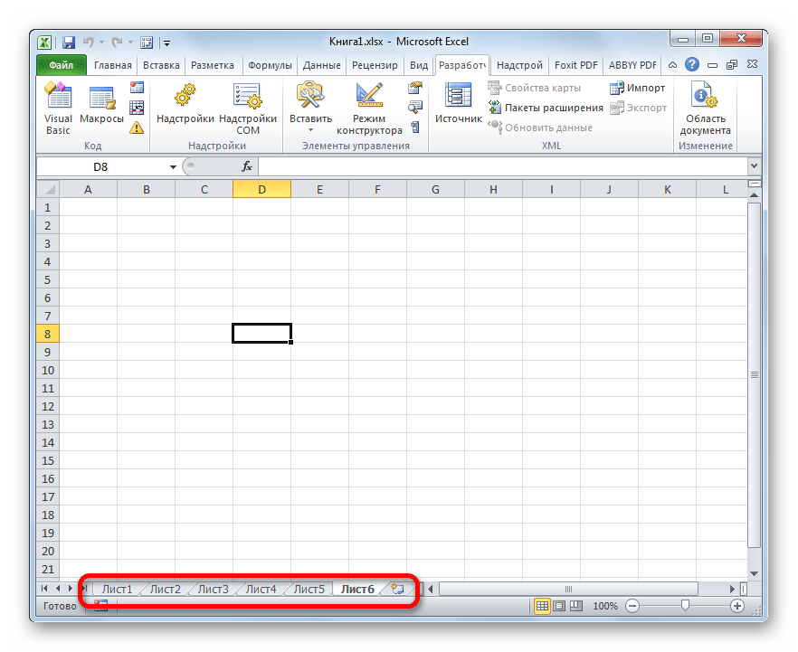
- Как видим, теперь все ярлычки отображаются на панели Excel.

Урок: Как включить или отключить макросы в Экселе
Способ 5: восстановление удаленных листов
Но, зачастую случается так, что ярлычки пропали с панели просто потому, что их удалили. Это наиболее сложный вариант. Если в предыдущих случаях при правильном алгоритме действий вероятность восстановления отображения ярлыков составляет 100%, то при их удалении никто такую гарантию положительного результата дать не может.
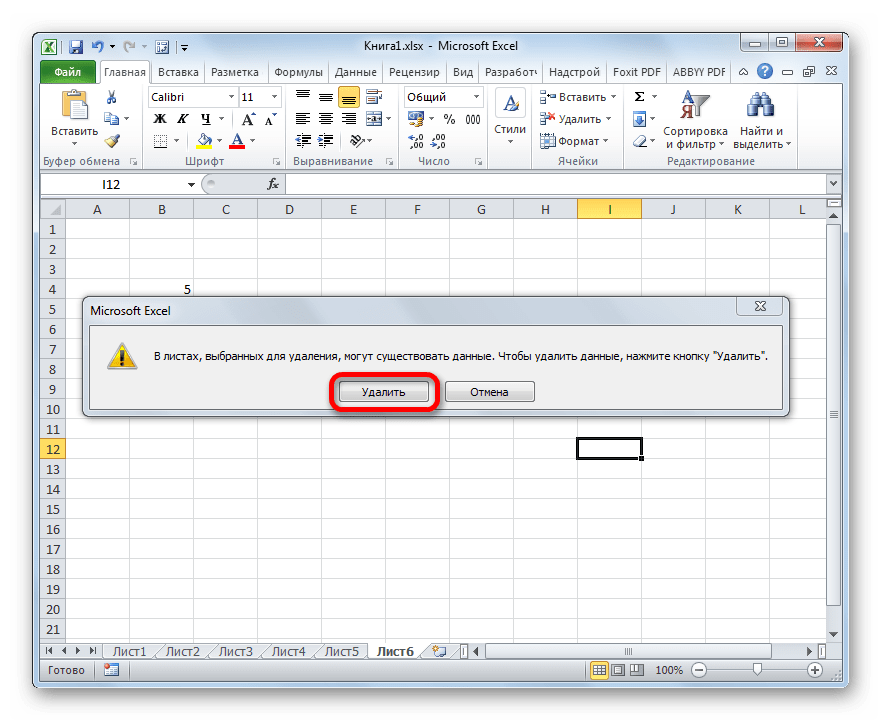
Удалить ярлык довольно просто и интуитивно понятно. Просто кликаем по нему правой кнопкой мыши и в появившемся меню выбираем вариант «Удалить».
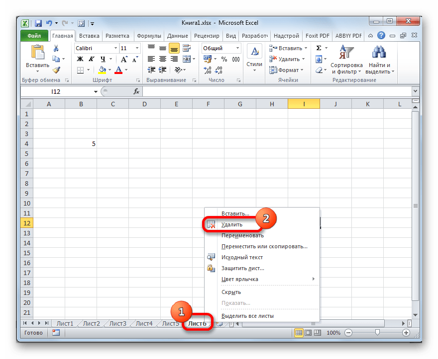
После этого появиться предупреждение об удалении в виде диалогового окна. Для завершения процедуры достаточно нажать на кнопку «Удалить».
Восстановить удаленный объект значительно труднее.
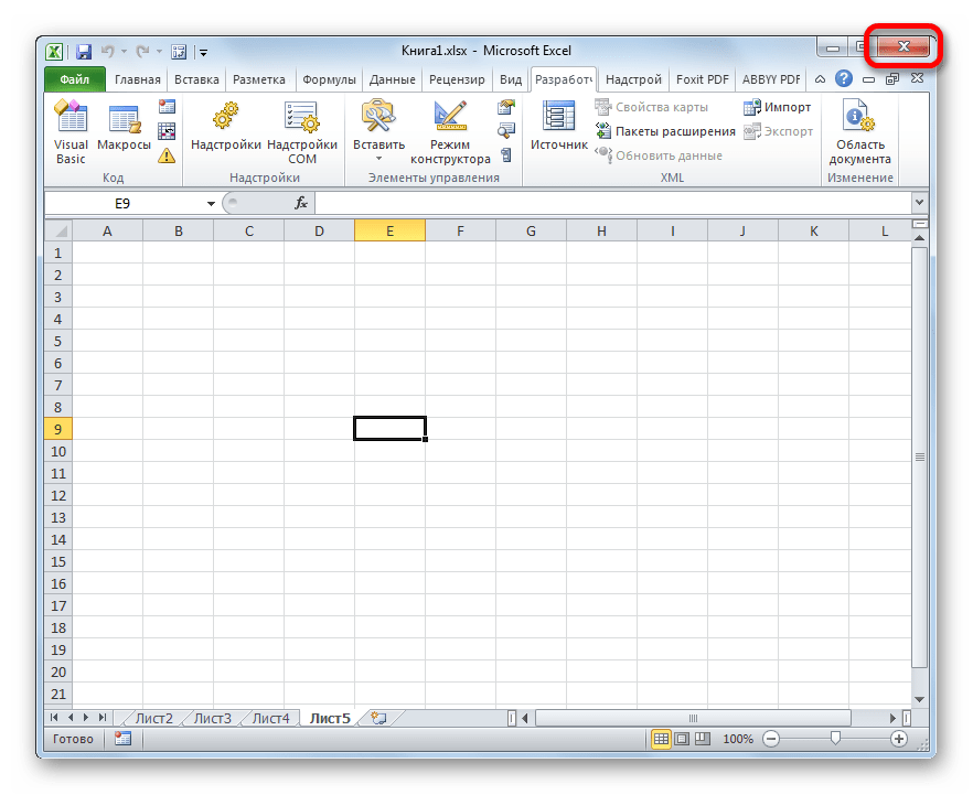
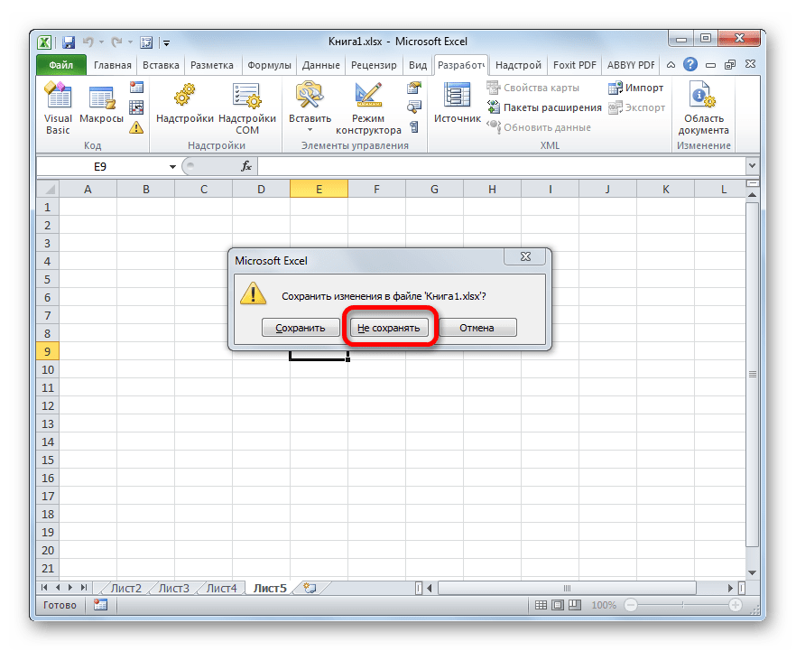
- Если вы уделили ярлычок, но поняли, что сделали это напрасно ещё до сохранения файла, то нужно его просто закрыть, нажав на стандартную кнопку закрытия документа в правом верхнем углу окна в виде белого крестика в красном квадрате.
- В диалоговом окошке, которое откроется после этого, следует кликнуть по кнопке «Не сохранять».
- После того, как вы откроете данный файл заново, удаленный объект будет на месте.
Но следует обратить внимание на то, что восстанавливая лист таким способом, вы потеряете все данные внесенные в документ, начиная с его последнего сохранения. То есть, по сути, пользователю предстоит выбор между тем, что для него приоритетнее: удаленный объект или данные, которые он успел внести после последнего сохранения.
Но, как уже было сказано выше, данный вариант восстановления подойдет только в том случае, если пользователь после удаления не успел произвести сохранение данных. Что же делать, если пользователь сохранил документ или вообще вышел из него с сохранением?
Если после удаления ярлычка вы уже сохраняли книгу, но не успели её закрыть, то есть, смысл покопаться в версиях файла.
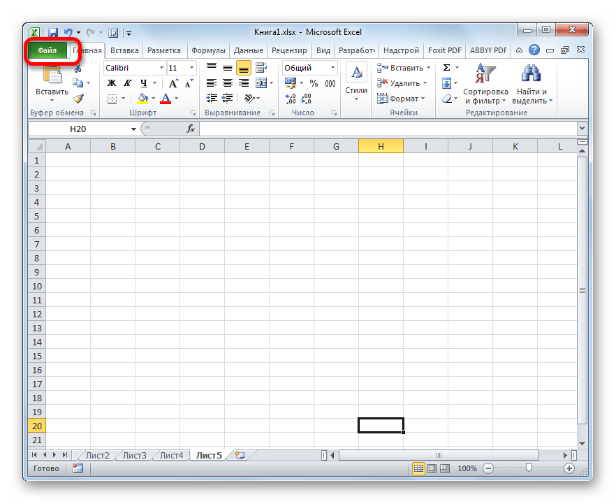
- Для перехода к просмотру версий перемещаемся во вкладку «Файл».
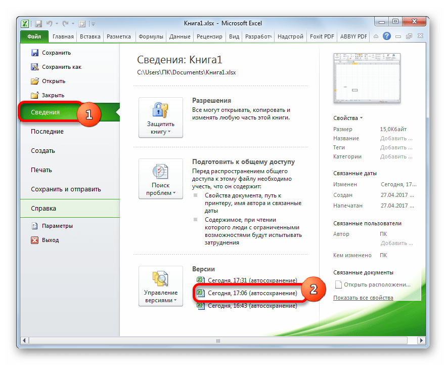
- После этого переходим в раздел «Сведения», который отображается в вертикальном меню. В центральной части открывшегося окна расположен блок «Версии». В нем находится список всех версий данного файла, сохраненных с помощью инструмента автосохранения Excel. Данный инструмент по умолчанию включен и сохраняет документ каждые 10 минут, если вы это не делаете сами. Но, если вы внесли ручные корректировки в настройки Эксель, отключив автосохранение, то восстановить удаленные элементы у вас уже не получится. Также следует сказать, что после закрытия файла этот список стирается. Поэтому важно заметить пропажу объекта и определиться с необходимостью его восстановления ещё до того, как вы закрыли книгу.
Итак, в списке автосохраненных версий ищем самый поздний по времени вариант сохранения, который был осуществлен до момента удаления. Щелкаем по этому элементу в указанном списке.
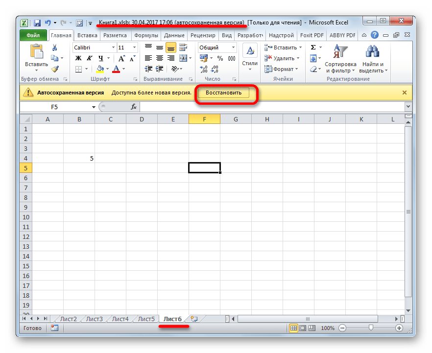
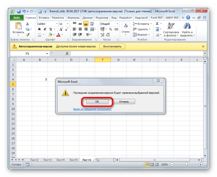
- После этого в новом окне будет открыта автосохраненная версия книги. Как видим, в ней присутствует удаленный ранее объект. Для того, чтобы завершить восстановление файла нужно нажать на кнопку «Восстановить» в верхней части окна.
- После этого откроется диалоговое окно, которое предложит заменить последнюю сохраненную версию книги данной версией. Если вам это подходит, то жмите на кнопку «OK».
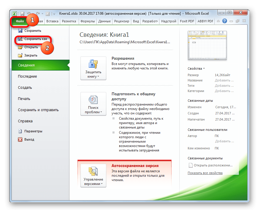
Если же вы хотите оставить обе версии файла (с уделенным листом и с информацией, добавленной в книгу после удаления), то перейдите во вкладку «Файл» и щелкните по пункту «Сохранить как…».
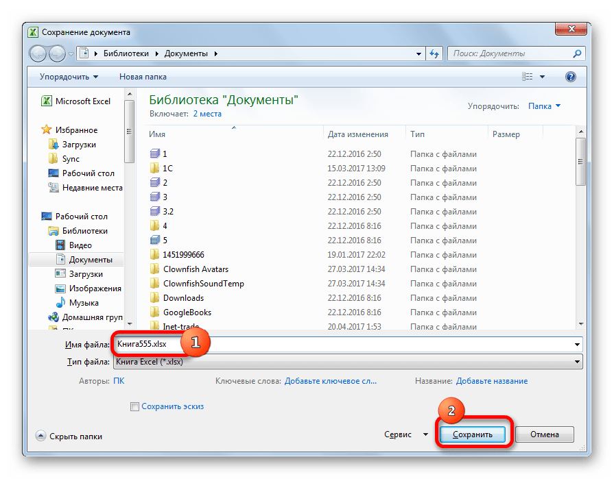
- Запустится окно сохранения. В нем обязательно нужно будет переименовать восстановленную книгу, после чего нажать на кнопку «Сохранить».
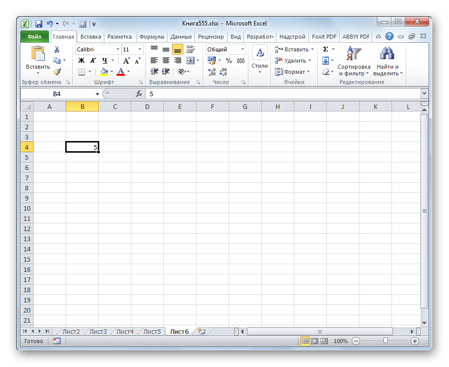
- После этого вы получите обе версии файла.
Но если вы сохранили и закрыли файл, а при следующем его открытии увидели, что один из ярлычков удален, то подобным способом восстановить его уже не получится, так как список версий файла будет очищен. Но можно попытаться произвести восстановление через управление версиями, хотя вероятность успеха в данном случае значительно ниже, чем при использовании предыдущих вариантов.
- Переходим во вкладку «Файл» и в разделе «Свойства» щелкаем по кнопке «Управление версиями». После этого появляется небольшое меню, состоящее всего из одного пункта – «Восстановить несохраненные книги». Щелкаем по нему.
- Запускается окно открытия документа в директории, где находятся несохраненные книги в двоичном формате xlsb. Поочередно выбирайте наименования и жмите на кнопку «Открыть» в нижней части окна. Возможно, один из этих файлов и будет нужной вам книгой содержащей удаленный объект.
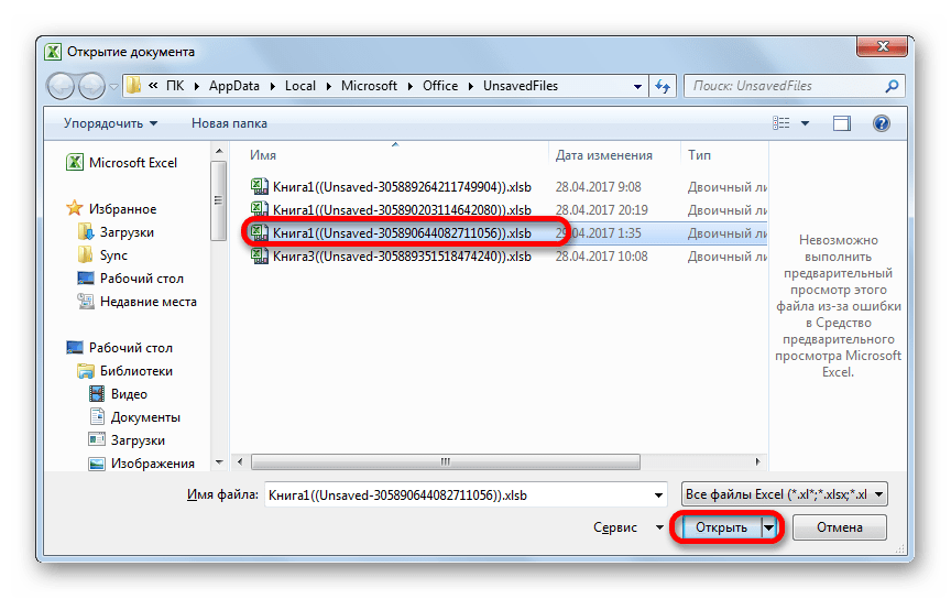
Только все-таки вероятность отыскать нужную книгу невелика. К тому же, даже если она будет присутствовать в данном списке и содержать удаленный элемент, то вполне вероятно, что версия её будет относительно старой и не содержать многих изменений, которые были внесены позже.
Урок: Восстановление несохраненной книги Эксель
Как видим, пропажа ярлыков на панели может быть вызвана целым рядом причин, но их все можно разделить на две большие группы: листы были скрыты или удалены. В первом случае листы продолжают оставаться частью документа, только доступ к ним затруднен. Но при желании, определив способ, каким были скрыты ярлыки, придерживаясь алгоритма действий, восстановить их отображение в книге не составит труда. Другое дело, если объекты были удалены. В этом случае они полностью были извлечены из документа, и их восстановление не всегда представляется возможным. Впрочем, даже в этом случае иногда получается восстановить данные.
One of the first “tricks” an Excel user learns is to hide and unhide a sheet.
This is an exceptionally useful feature as it allows us to store data in a sheet, such as lists and tables, but keep the user of the workbook from seeing, manipulating, and more importantly, corrupting the information on the hidden sheet.
As with most things in Excel, there is more than one way to hide a sheet or multiple sheets. One of the easiest methods is to select a sheet (or select multiple sheets using standard Windows CTRL and Shift selection techniques), right-click the sheet tab then select “Hide”.

As an example; suppose you have twelve sheets labeled “January” through “December” and you want to hide all the monthly sheets except “December”.
- Select the “Jan” sheet
- Hold down the Shift key
- Select the “Nov” sheet
- Right-click on any selected sheet tab
- Click “Hide”

Unfortunately, unhiding multiple sheets in a single step is not as easy. If you right-click a sheet tab and select “Unhide”, the proceeding dialog box only allows a single sheet to be selected for the unhide operation.

This means you will have to perform the unhide operation eleven times to restore all the hidden sheets to a visible state.
Never fear, a solution is here (actually, three solutions)
Solution 1 – Create a Custom View
An often-overlooked feature in Excel is the ability to save a custom view.

Custom views can be used to “save” the hidden or visible states of rows and columns. This is convenient when you wish to show details of data for one printout, but a summarized version of the data in a different printout.
- Hide the desired rows and/or columns.
- Click View (tab) -> Workbook Views (group) -> Custom Views -> Add… and give the current configuration a name.

If you change the hidden/visible state of rows and/or columns but then wish to return to the saved configuration, repeat the process (View (tab) -> Workbook Views (group) -> Custom Views), select your saved view then click “Show”.

The screen will immediately return to the desired state.
Custom views also work with the visible/hidden states of worksheets. If we create a custom view prior to hiding ANY of the sheets (View (tab) -> Workbook Views (group) -> Custom Views -> Add…), we can hide as many sheets as we like. When it comes time to redisplay all the sheets, we repeat the process and select our “normal” view and click “Show”.
All the sheets have returned.
There is one negative to this process. Custom views do not work with Data Tables. The moment you add a Data Table to ANY sheet, the Custom Views feature becomes inoperable.

Because more and more people use Data Tables in their workbooks (and why wouldn’t you? They’re AMAZING!!!), we need to explore another way of unhiding all hidden worksheets.
Solution 2 – Using the VBA Immediate Window
Right up front, this does not require the use of macro-enabled workbooks. This technique can be performed in any Excel workbook.
- Open the Visual Basic Editor by pressing Alt-F11 on the keyboard or right click on any sheet tab and select View Code.

Don’t concern yourself with what you see in the ensuing window; all of that is for another day.
- Activate the Immediate Window by clicking View -> Immediate Window (or CTRL-G).

Now we will run a macro. This macro will loop through all the hidden sheets and revert their visibility states to “visible”. We will use a “For…Each” collection loop to perform this operation.
NOTE: If you are interested in learning about this command and many other useful things macros can do for you, visit the links at the end of this tutorial.
- In the Immediate window, type
for each sh in worksheets: sh.visible=true: next sh
(press Enter)
All the sheets have returned to a visible state.

What does that code mean? Let’s break down the code.
for each sh in worksheetsThis establishes a collection (list) of all worksheets and allows us to refer to each sheet individually with the alias “sh”.
sh.visible=trueWith the first sheet in the collection, set the visible property to “true”. This makes the sheet visible to the user.
next shThis selects the next sheet in the collection and returns to the first statement to repeat the process.
This process will repeat for as many sheets as are in the collection.
If this code is something you will use frequently, you can save the code in a Notepad file and then copy/paste it back into the Immediate Window whenever needed.
Solution 3 – Add a Macro to the Quick Access Toolbar (QAT)
This technique is covered in detail in the Excel VBA course (link below if you are interested in becoming a VBA Powerhouse) but will be summarized here.
If this feature is to be used often across many different workbooks, it’s worth taking the time to set this feature up on the QAT.
We will create a simple macro and store it in a special place in Excel called the Personal Macro Workbook.
Creating the Macro
- Click the “Record Macro” button on the Status Bar in the lower-left corner of Excel.
- Give the macro a name (“Unhide_All” is a good name.) Macro names cannot contain spaces.
- Change the “Store macro in:” option from “This Workbook” to “Personal Macro Workbook”.
- Click OK
- Click the “Stop Recording” button on the Status Bar in the lower-left corner of Excel.
- Open the Visual Basic Editor (Alt-F11).
- In the Project Explorer panel (upper-left), click the plus-sign next to the entry labeled “VBAProject (PERSONAL.XLSB)”.
- Click the plus-sign next to the folder labeled “Modules”.
- Double-click the module named “Module1”.
- Highlight and delete EVERYHTING in the code window (right panel).
- Enter the following code:
Sub Unhide_All()
Dim sh As Worksheet
	for each sh in worksheets: sh.visible=true: next sh
End Sub
Setting up the QAT Macro Launch Button
- Click the down arrow at the far right of the QAT and select “More Commands…” towards the bottom of the list.
- In the dropdown titled “Choose commands from:” select “Macros”.
- Select the “Unhide_All” macro on the left and click “Add>>” to move the macro to the list on the right.
- Click the “Modify” button to personalize the button icon as well as provide a tooltip. Whatever you write in the “Display name:” filed will appear on the screen when the user hover’s over the launch button on the QAT.
- Click OK.
Whenever you want to invoke the macro to unhide all the hidden sheets, click the unhide macro button on the QAT.

This feature is available for use in all open workbooks. Because we have updated the Personal Macro Workbook, don’t forget to save the changes to the Personal Macro Workbook when closing Excel.

Additional Resources
Excel VBA For…Each Loop tutorial
Excel VBA – Full Playlist
If you don’t have Office 365 and you’d like a free tool that unhides all sheets for you, then this is it!
You can add this tool to your Quick Access Toolbar or to your Excel ribbon by saving it in your Personal Macro Workbook. In this video I show you the steps to do that.

Many Thanks to Daniel Lamarche from Combo Projects for sharing this tool for free with our community members.
Please visit Daniel’s page at:
Published on: March 7, 2019
Last modified: March 2, 2023


Leila Gharani
I’m a 5x Microsoft MVP with over 15 years of experience implementing and professionals on Management Information Systems of different sizes and nature.
My background is Masters in Economics, Economist, Consultant, Oracle HFM Accounting Systems Expert, SAP BW Project Manager. My passion is teaching, experimenting and sharing. I am also addicted to learning and enjoy taking online courses on a variety of topics.
One of my customers, faced the following strange problem when he opens several Excel files: The Excel file seem to open normally, but the Excel won’t show the worksheet (Worksheet area is grayed out and the data doesn’t appear at all). As a first try, I repaired the MS Office (2007) installation but the problem still exists. Finally after some research I found the following solution to resolve the «Excel Worksheet data not showing» problem.
How to fix: Excel Data not showing – not visible – data area is grayed out.
1. Go to View Menu and ensure first that the Unhide option is inactive. (otherwise click Unhide and check if you can view the excel data).
2. Select Arrange All.

3. At the menu that comes up, check the «Windows of active workbook» checkbox and click OK.

Now you should see the contents of the Excel Workbook!
4. One last action. Save the Workbook and you ‘re done!
Additional help: If the above tip doesn’t help you, then:
A. Perform a repair at Office installation. To do that:
- Navigate to Windows Control Panel > Programs and features.
- Locate and select the MS Office application and then click Change.
- Then select the Repair option.
B. Disable the Hardware Acceleration at Excel application: To do that:
Notice: The option to disable the graphics acceleration is only available at Excel 2010 and Excel 2013.
1. From Excel’s main menu select Options.

2. At Excel Options window, choose Advanced on the left pane.

3. At the right pane, under Display options, uncheck the «Disable hardware graphics acceleration» checkbox and click OK.

That’s all folks! Did it work for you?
Please leave a comment in the comment section below or even better: like and share this blog post in the social networks to help spread the word about this solution.
If this article was useful for you, please consider supporting us by making a donation. Even $1 can a make a huge difference for us.

Did you know that Excel has two levels of hidden worksheets? Excel has “hidden” worksheets, and, “very hidden” worksheets. This post walks through the differences, and how to hide worksheets at each level.
By default, all new worksheets are visible. A visible worksheet’s tab appears in the bottom of the Excel window, enabling the user to click the tab in order to navigate to the worksheet. Easy enough, let’s move on.
Visible Property
In the real world, an object is either visible or it is not. For example, Harry Potter is typically visible. However, when he throws on that sweet cloak of invisibility, he is not visible. His visible status changes to false. In the real world, the visible status of an object is either true or false, it is either visible or it is not. In Excel however, the visible property of a worksheet object has three possible values: true, false, or….very hidden.
Hidden
When a worksheet has a visible property value of true, it is visible and can be seen and selected by the user. When a worksheet has a visible property of false, it is hidden, and can no longer be seen from within the standard Excel user interface. That is, the sheet’s tab is gone. The sheet itself however, is not gone, and formulas can still retrieve values stored on a hidden sheet. It just disappears from the user interface.
It is pretty easy to hide a sheet. Although, if we are trying to be technical, we should say it this way: it is pretty easy to change a worksheet’s visible property from true to false.
All five worksheets in my workbook are visible in the following screenshot.
![]()
To hide a sheet, simply right-click the sheet’s tab and select hide. You can also hide a sheet using the following ribbon command:
- Home > Format > Hide & Unhide > Hide Worksheet
You can also hide a sheet using the following keyboard shortcut:
- Alt+o, h, h
Sheet2 is hidden in my workbook, as shown in the screenshot below:
![]()
To unhide a sheet, simply right-click any sheet’s tab and select Unhide. This reveals the Unhide dialog box as shown below.
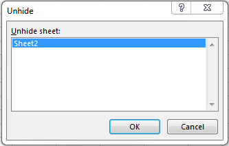
Pick the hidden sheet and click ok. You can also unhide a sheet using the following ribbon command:
- Home > Format > Hide & Unhide > Unhide Worksheet
You can also unhide a sheet using the following keyboard shortcut:
- Alt+o, h, u
Now, here is where it gets fun, creating very hidden sheets.
Very Hidden
The third property value is very hidden. The difference between a hidden sheet and a very hidden sheet is simply this: very hidden sheets do not appear in the Unhide dialog box.
Now, before we get to the mechanics of how to set a sheet’s property to very hidden, let me set up a bit of background that will be useful. First, we need to understand that in Excel, there is a world outside of the typical Excel user interface. What you see when navigating inside the Excel application window is a subset of everything available in Excel. A primary example is macros. Macros are not edited within the standard interface, they are edited within a utility application called the Visual Basic Editor (VBE). The VBE is a powerful and useful utility, and Excel power users spend quite a bit of time in it. It is inside the VBE where we change the visible property of a worksheet to very hidden. Here is how the VBE refers to the Visible property values:
- True = xlSheetVisible
- False = xlSheetHidden
- Very Hidden = xlSheetVeryHidden
You still with me? Great, let’s get into the VBE now.
Visual Basic Editor
There are a couple of different ways to open the VBE. You could use either of the following keyboard shortcut:
- Alt+F11
- Alt+t, m, v
Or, if you are more of a ribbon person, you could use the following ribbon command:
- Developer > Visual Basic [Note: Microsoft does not ship Excel with the Developer ribbon tab visible, so, you’ll need to turn it on. In Excel 2010/2013: customize the ribbon and check the Developer tab. In Excel 2007: go into options and check the “Show developer tab in ribbon” checkbox]
At this point, you should have the VBE open, and it should look a little something like the screenshot below.

In the top left panel is the Project Explorer, where you can use the tree to navigate to any open workbook, and to any sheet. Double-click the sheet you want to update.
[Note: if you don’t see the Project Explorer, simply select View > Project Explorer]
Then, you’ll be able to view and change the status of the Visible property in the Properties window.
[Note: if you don’t see the Properties window, simply select View > Properties Window]
On the Visible property, use the combo box to change the value to xlSheetVeryHidden, or, to either of the other options.
In the screenshot below, I selected xlSheetVeryHidden from the Visible property combo box:
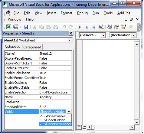
Once you return to Excel, you’ll notice that the sheet’s tab is not visible. You’ll also notice that if the workbook contains very hidden sheets, the user won’t have an option to open the Unhide dialog box. If the workbook contains both hidden and very hidden sheets, then the user can open the Unhide dialog box, however, the very hidden sheets do not appear. In my workbook, Sheet2 is very hidden, and Sheet3 is hidden, and the Unhide dialog box is shown in the screenshot below.
Wow, Sheet2 is very hidden!
If you want to view the sheet again, simply change the property from xlSheetVeryHidden to xlSheetVisible from within the VBE and you’ll be all set.
Now, with great power comes great responsibility, so use this super power with great care!